Cracks in rubber under tension exceed the shear wave speed

Abstract

The shear wave speed is an upper limit for the speed of cracks loaded in tension in linear elastic solids. We have discovered that in a non-linear material, cracks in tension (Mode I) exceed this sound speed, and travel in an intersonic range between shear and longitudinal wave speeds. The experiments are conducted in highly stretched sheets of rubber; intersonic cracks can be produced simply by popping a balloon.

Cracks advance by consuming the potential energy stored in the surrounding elastic fields and, thus, one expects that they should travel no faster than the speed of sound. While this intuition is indeed correct, solids support longitudinal, shear, and surface (Rayleigh) waves, with distinct speeds $c_{L}>c_{s}>c_{R}$, respectively Achenbach (1973), and determining which of these is the upper limit for crack speeds is a subtle problem.

In the case of linear elastic solids, Stroh was first to argue that cracks loaded in tension (Mode I) could not exceed the Rayleigh wave speed $c_{R}$ Stroh (1957). The mathematical analysis of Freund and others Freund (1990); Broberg (1999) showed that the energy consumed by a crack diverges as its speed approaches $c_{R}$, suggesting that cracks cannot travel faster than this speed. However, geological field measurements of fault motion Heaton (1990), computer simulations Andrews (1976); Gao et al. (2001), and laboratory experiments Rosakis (2002) have established that cracks loaded in shear (Mode II) can exceed $c_{s}$ (and hence $c_{R}$) and reach speeds close to $c_{L}$. Dynamic fracture theory was extended to include these “intersonic” cracks Burridge et al. (1979); Broberg (1999); Ranjith and Rice (2001). However, even when revisited in light of the arguments that allowed intersonic cracks in shear-loaded samples, linear elastic fracture mechanics forbids intersonic cracks loaded in tension Broberg (1999).

In the case of elastic materials subjected to large deformations, it is natural to assume that the crack speed is bounded above by the shear wave speed. Recent numerical simulations have found mode I cracks running faster than this wave speed Buehler et al. (2003). Here we present experimental results which show crack speeds faster than the shear wave speed occur in popping rubber.

Experiment. Our experiments are conducted with sheets of natural latex rubber 0.15 mm thick purchased from McMaster-Carr, stretched biaxially in a tensile testing machine, and punctured by pricking the sheet with a needle. The samples are rectangular, 12.7 cm wide and 27.9 - 34.3 cm long, depending on the expected maximum extension, and their perimeter is divided into tabs 3.0 cm wide that serve as gripping points for the testing apparatus. A square grid is drawn on the sample to monitor the magnitude and homogeneity of extension as the sample is stretched.

The apparatus consists of two fixed and two mobile linear guide rails (see Fig. 1(a)). The mobile rails move independently and orthogonally. Multiple sliding clamps that grip individual tabs on the sample are mounted on each rail. The sheet was attached to these clamps and stretched to an extension state ($\lambda_{x}$,$\lambda_{y}$) such that $\lambda_{y}>\lambda_{x}$, where $\lambda_{i}$ is the ratio of the stretched to original length along the $i$ direction, and $x$ and $y$ are the long and short directions, respectively. As the rails are moved apart, the sheet expands and the clamps separate by sliding along the rail, yet remain equidistant due to the elastic coupling to each other through the sheet.

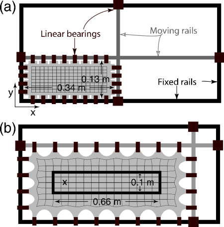
Figure 1: Apparatus for creating biaxial extensions in a thin rubber sheets. (a) Initial state of the sample loaded in the test apparatus. (b) Final state of the sample after extension. The dark rectangle is a rigid frame attached to the sample and the ‘$\times$’ marks the crack initiation.

After reaching the desired extension state, the sheet is clamped between two steel rectangular frames (10.2 cm $\times$ 66 cm)(Fig. 1(b)). Then the extension state of the sheet is fixed and determined exclusively by these clamping frames. The frames fix the total energy available to the crack, and since the aspect ratio is small, the crack will consume equal amounts of energy per crack length Rice (1967).

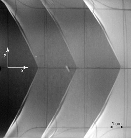
Figure 2: Multiple exposure photograph of a crack in a rubber sample ($\lambda_{x}=2.2,\lambda_{y}=3.2$). The exposures, separated in time by 500 $\mu$s, are captured on a single frame with a CCD camera.

A crack is initiated by pricking the sheet with a pin at the point marked ’$\times$’ in Fig. 1(b) and the velocity is determined photographically. Along the expected crack path we position an optical sensor that triggers a strobing flash when the crack parts the rubber blocking the beam path of the sensor. A CCD camera captures multiple images from each flash pulse on a single frame producing an image as shown in Fig. 2. As reported in Deegan et al. (2002), the crack can run straight or wavy depending on the extension state; irrespective of the crack path, the velocity of the crack, $v_{c}$, is calculated by the distance between successive crack tip positions and the time interval between flashes. Cracks are wavy for $\lambda_{x}>2.2$. These measurements are reproducible within 5% from trial to trial.

Longitudinal wave speed. We also measure the longitudinal speed for infinitesimal amplitude waves along the $x$ direction in rubber as a function of $\lambda_{x}$ and $\lambda_{y}$. In rubber, sound speeds vary strongly with the degree of extension due to nonlinear strain-extension relation and large deformations. In particular, when $\lambda_{x}\neq\lambda_{y}$, the sound speed depends on the direction. We use a time-of-flight method because standard ultrasonic techniques for measuring sound speeds are difficult to implement. The sheet is first stretched to an extension state $\lambda_{y}>\lambda_{x}$. Two record needles (marked by ’+’ in Fig. 3(a)) are placed in contact with the sheet about 5 cm apart along the $x$ direction. A bar is attached across the $y$ direction of the sheet about 5 cm from the first needle. The bar is attached to a speaker and an in-plane, $x$–directed perturbation is applied to the sheet by pulsing the speaker. The signals from the record needles are recorded with a digitizing oscilloscope, and the longitudinal speed in the $x$ direction is calculated from the time lag between the separate signals and the known distance between the needles. Note that the speed is that of a linear wave moving on the stretched material; i.e., we are measuring the propagation speed of small distortions around the stretched state.

We have been unable to measure the shear wave speed directly due to the thinness of the material, which makes it difficult to excite shear waves. Instead we measure the appropriate force-extension curve and calculated the velocity from it. As a proof-of-principle, we have calculated in this manner the longitudinal wave speed. We measure the force vs. displacement curve for the configurations depicted in Fig. 3(b). The material is stretched to the state ($\lambda_{x}$,$\lambda_{y}$), a long but narrow portion is gripped along the long edges, and one of the grips is oscillated sinusoidally at $f=25$ Hz in the $x$ direction while the other was fixed. A load cell and accelerometer attached to the driven clamp measures the applied force $F$ and acceleration $a$. The displacement $\delta x=a/(2\pi f)^{2}$ follows by integration.

Since the measurement is in a strip narrow compared to its length, departures of the strain in the $y$ direction from the stretched state $\epsilon_{yy}$ is zero almost everywhere. This state of strain corresponds to the state excited by a longitudinal wave in a thin sheet: only $\epsilon_{xx}$ and $\epsilon_{zz}$ are nonzero. Therefore, the force and displacement measurements in this configuration yield the modulus needed to calculate $c_{L}$: $Y=FW/(\delta xLd)$ where $W$ is the distance between the grips, $L$ is the length of the grips, $d$ is the thickness of the material in the stretched state, and the longitudinal wave speed along the $x$ direction is $c_{L}=\sqrt{Y/\rho}$, where $\rho=944$ kg/m³ is the mass density of the sheet.

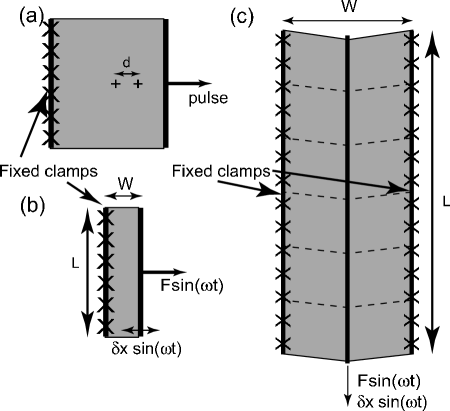
Figure 3: Experimental configurations for determining sound speeds: (a) direct measurement of the longitudinal wave speed using a time-of-flight method; indirect determination of (b) the longitudinal wave speed and (c) the shear wave speed from a force-displacement measurement. In each setup, the sheet is first brought to the desired state of extension ($\lambda_{x},\lambda_{y}$), the fixed and movable clamps are attached to the sheet, and the measurements proceed.

The ratio of the measured to calculated wave speed is plotted in Fig. 4 for $\lambda_{y}=3.2$ and $\lambda_{x}$ varying between 2 and 3.2. For perfect agreement this ratio should be 1. The data points lie within experimental error of this value, validating the procedure for calculating the wave speed from the force-displacement relationship.

Shear wave speed. The configuration in Fig. 3(c) is used to measure the shear modulus, $G=FW/(4Lt\delta x)$, from which we calculate the shear wave speed in the $x$ direction, $c_{S}=\sqrt{G/\rho}$. A rubber sheet is stretched to $\lambda_{y}>\lambda_{x}$, and a long narrow rubber strip is gripped on opposite edges, as shown. A thin bar down is glued to the center line of the strip and oscillated in the $y$-direction. The result for $G$ obtained from the force and acceleration measurements then yields $c_{s}$.

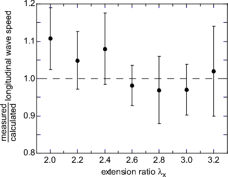
Figure 4: The ratio of measured to calculated longitudinal wave speed plotted as a function of $\lambda_{x}$ for fixed $\lambda_{y}=3.2$.

Material frame. It is interesting to examine our data in the material (Lagrangean) frame rather than the lab (Eulerian) frame because, as we show below, in the material frame the shear wave speeds are completely isotropic. In the material frame, length is measured in units of a coordinate system that deforms with the material: for biaxial deformation $(\lambda_{x},\lambda_{y})$, the relation between velocity in the material frame $\mathbf{c}^{(m)}$ and the stretched (or lab) frame $\mathbf{c}^{(s)}$ is $\mathbf{c}^{(m)}=(c^{(m)}_{x},c^{(m)}_{y})=(c^{(s)}_{x}/\lambda_{x},c^{(s)}_{y}/\lambda_{y})$.

Results. In Figure 5 we compare crack speeds with wave speeds as a function of $\lambda_{x}$ for $\lambda_{y}=3.2$. The data indicate cracks travel 10-20% faster than the shear wave speed, but slower than the longitudinal sound speed. We adopt here the descriptor “intersonic” used in studies of shear loaded cracks, for cracks that travel at speeds between the longitudinal and shear wave speeds.

Discussion There are some natural questions to ask concerning choices made in Fig. 5. (1) When rubber is stretched the wave speed is anisotropic. Why did we choose just to plot the wave speeds in the $x$ direction? (2) Large amplitude deformations typically travel at speeds different from those of infinitesimal amplitude waves. Why can we use small amplitude speeds as a basis for comparison?

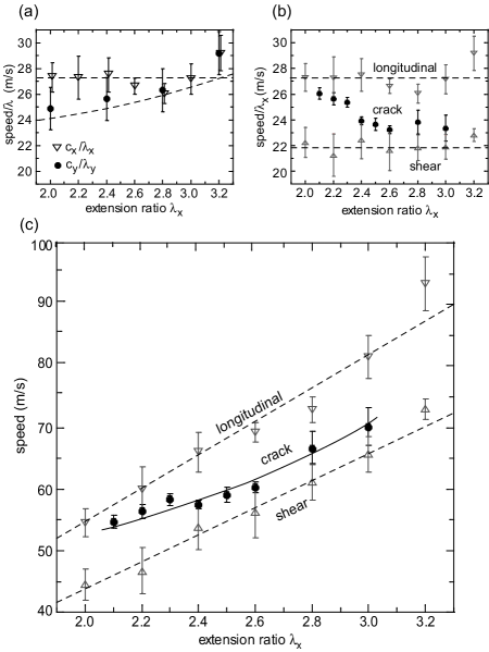
Figure 5: Comparison of measured longitudinal and shear wave speeds as a function of $\lambda_{x}$ at fixed $\lambda_{y}=3.2$ with Mooney-Rivlin theory (dashed lines). (a) $x(\triangledown)$ and $y(\bullet)$ direction longitudinal wave speeds in the material frame. (b) Longitudinal wave speed ($\triangledown$), crack speed ($\bullet$), and shear wave speed ($\triangle$) in the material frame. (c) Longitudinal wave speed ($\triangledown$), crack speed ($\bullet$), and shear wave speed ($\triangle$) in the lab frame.

The answers to these question stem from the fact that our rubber samples are described accurately by the Mooney-Rivlin theory, which we now summarize. Any continuum theory of deformation that depends upon relative motion of neighboring mass points can only involve particle displacements $\mathbf{x}(\mathbf{X})$ through the strain tensor $E_{\alpha\beta}=(1/2)[\sum_{\gamma}(\partial x_{\gamma}/\partial X_{\alpha}\partial x_{\gamma}/\partial X_{\beta})-\delta_{\alpha\beta}]$. Here $\mathbf{x}(\mathbf{X})$ describes the location in space of a mass point originally at $\mathbf{X}$. A two–dimensional isotropic theory can only depend upon the strain tensor through the two invariant quantities $I_{1}=E_{xx}+E_{yy}$ and $I_{2}=E_{xx}E_{yy}-E_{xy}^{2}$. Under biaxial strain $E_{ii}=(\lambda_{i}^{2}-1)/2$. In the Mooney-Rivlin Theory Mooney (1940); Rivlin (1948); Klingbeil and Shield (1966), the strain energy density of a thin sheet of rubber is given by

$$W=a\big{(}I_{1}+bI_{2}\big{)}$$ (1)

In the material or Lagrangean frame a calculation of the longitudinal and shear wave speeds yields:

$$\rho c^{(m)2}_{xl}=a[1+\frac{b}{2}(\lambda_{y}^{2}-1)]$$ (2)

$$\rho c^{(m)2}_{yl}=a[1+\frac{b}{2}(\lambda_{x}^{2}-1)]$$ (3)

$$\rho c^{(m)2}_{xs}=a(1-\frac{b}{2})$$ (4)

To recover the speed in the lab or Eulerian frame $\mathbf{c}^{(s)}=(c^{(s)}_{x},c^{(s)}_{y})=(\lambda_{x}c^{(m)}_{x},\lambda_{y}c^{(m)}_{y})$. From these equations we see that the longitudinal and shear wave speeds in the $x$ direction are independent of $\lambda_{x}$ and that the $y$ direction longitudinal wave speed increases monotonically with increasing $\lambda_{x}$, both of which we observe. More importantly, $c^{(m)}_{s}$ is independent of direction. With the value of $a=501$ (m/s)² and $b=0.106$, all our sound speed data are well characterized by these equations, as is shown by the dashed lines in Fig. 5.

Furthermore, in Mooney-Rivlin materials, speeds of infinitesimal longitudinal and shear waves are exactly equal to the finite amplitude plane wave speeds. Therefore, although we are measuring small amplitude wave speeds, these speeds bound the speed of any finite amplitude plane wave deformation. Thus, it is appropriate to compare the wave speeds we measured to crack speeds.

Lastly, we note that when a moving object travels in an elastic medium faster than the wave speed, it creates a shock wave in the form of a Mach cone. The wedge-like crack opening typical of cracks in rubber (shown in Fig. 2) is strikingly similar to the Mach cone, suggesting that rubber cracks are shock-like, exceeding some response speed of the medium. Shock waves are known to form when finite tensile pulses travel in pre-stretched rubber strips Kolsky (1969).

Conclusion. In earlier work we found that cracks in rubber follow oscillating paths when the horizontal extension exceeds a critical value. We still have no good explanation for this dynamical transition. However, knowing that the fractures travel above the shear wave speed will be important in resolving this question.