Entanglement in a Noninteracting Mesoscopic Structure

Abstract

We study the time dependent electron-electron and electron-hole correlations in a mesoscopic device which is splitting an incident current of free fermions into two spatially separated particle streams. We analyze the appearance of entanglement as manifested in a Bell inequality test and discuss its origin in terms of local spin-singlet correlations already present in the initial channel and the action of post-selection during the Bell type measurement. The time window over which the Bell inequality is violated is determined in the tunneling limit and for the general situation with arbitrary transparencies. We compare our results with alternative Bell inequality tests based on coincidence probabilities.

I Introduction

Quantum entanglement of electronic degrees of freedom in mesoscopic devices has attracted a lot of interest recently. The first proposal to probe localized entangled electrons through transport and noise measurements loss soon lead to specific structures which generate spatially separated streams of entangled particles ent_sc ; ent_qd . One class of devices makes use of a superconducting source emitting Cooper pairs into a normal-metal structure with two leads in a fork geometry: entanglement has its origin in the attractive interaction binding the electrons into Cooper pairs, while the spatial separation of correlated electrons is arranged for by suitable ‘filters’ ent_sc . Another class of devices makes use of Coulomb interactions in confined geometries ent_qd . All of these proposals involve electronic spins as the entangled quantum degrees of freedom; an alternative scheme has been pointed out by Samuelsson et al. samuelsson_03 who propose a setup where real space orbital degrees of freedom become entangled. Besides these proposals for the generation of spatially separated entangled pairs, the implementation of Bell inequality tests probing their entanglement has been discussed in detail kawabata_01 ; chtchelkatchev_02 ; samuelsson_03 . The combination of sources for the creation and methods for testing the correlations of entangled particle streams are first steps towards establishing this quantum resource for solid state based quantum information technology.

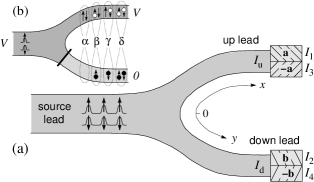
Figure 1: (a) Mesoscopic normal-metal structure in a fork geometry generating two streams of spin-correlated electrons in the two arms of the fork. The Bell type setup detects spin-currents $I_{i}$, $i=1,3$, projected onto the directions $\pm{\bf a}$ in the upper arm and correlates them with spin-currents $I_{j}$, $j=2,4$, projected onto the directions $\pm{\bf b}$ in the lower arm. (b) In the tunneling limit (with a small transparency $T_{\mathrm{d}}\ll 1$ in the ‘down’ arm) a fraction of spin-entangled electrons is split into the two arms (components $\beta$ and $\gamma$); their correlations can be efficiently measured in a Bell type setup sensitive to hole (electron) currents in the ‘up’ (down) lead.

An interesting proposal has recently been made by Beenakker et al. beenakker_03 (see also Ref. beenakker_03b, and the note note, ): using a two-channel quantum Hall device with a beam splitter, they suggest a setup generating two streams of entangled electron-hole pairs and confirm the presence of correlations through a Bell inequality (BI) test. A crucial difference to previous proposals is the absence of interactions generating the entanglement (see also Refs. note, ; fazio_03, ; ssb_04, ). In this paper, we investigate a similar setup involving a mesoscopic normal-metal structure arranged in a fork geometry and generating two streams of correlated electrons in the two arms of the fork, see Fig. 1. In our formulation of the Bell inequalities we take special care to use only directly measurable observables. We find that a Bell inequality test involving correlations between the electronic spin-currents in spatially separated leads exhibits violation at short time scales $\tau<\tau_{\rm\scriptscriptstyle BI}$, with $\tau_{\rm\scriptscriptstyle BI}$ given by the single particle correlation time $\tau_{V}=\hbar/eV$. We show, that the time $\tau_{\rm\scriptscriptstyle BI}$ can be considerably extended in the tunneling limit, where the propagation into one of the arms (we choose the ‘down’ lead in Fig. 1) is strongly reduced by a small transparency $T_{\mathrm{d}}$. This small transparency can be exploited by a suitable choice of the observables in the Bell inequality test: going over to hole currents in the well conducting ‘up’ lead, we find the long violation time $\tau_{\rm\scriptscriptstyle BI}=\tau_{V}/\sqrt{T_{\mathrm{d}}}$. We also analyze an alternative Bell inequality based on coincidence probabilities derived from electron-hole number correlators and find it violated on even longer times $\tau_{\rm\scriptscriptstyle BI}=\tau_{V}/T_{\mathrm{d}}$. When tracing the origin of these BI violations, we find that the fermionic statistics already enforces the injection of spin-singlet correlated electron pairs with correlations extending over the distance $v_{\rm\scriptscriptstyle F}\tau_{V}$ with $v_{\rm\scriptscriptstyle F}$ the Fermi velocity. In addition, the splitting of this pair and a subsequent post-selection shih_88 ; ssb_04 in the Bell type measurement are crucial steps in rendering the original spin-entanglement amenable to observation and potentially useful as a resource of entangled quantum degrees of freedom.

In the following, we first analyze (Sec. II) the two-particle density matrix of the injected particle stream and find it to be locally singlet correlated; the extension to the scattered state behind the beam splitter demonstrates that this entanglement is preserved. We proceed with a discussion of Bell inequality measurements (Sec. III) and compare two types of Bell parameters, one based on current cross-correlators and a second one starting from coincidence probabilities, i.e., particle number correlators. We then turn to the actual calculation of the finite time spin-current correlators and their combination into the Bell parameter (Sec. IV). Results are presented for Bell inequalities involving electron-electron (general case) and electron-hole (tunneling limit) current correlations as well as for the corresponding expressions based on coincidence probabilities; we demonstrate that the violation of the Bell inequality depends sensitively on the choice of observables. Finally, we present our conclusions in Sec. V.

II Two-particle correlations

In order to analyze the properties of the injected electrons, we determine the two-particle density matrix (or pair correlation function) within the source lead,

$$g_{\vec{\sigma}}(x,y)={\rm Tr}\bigl{(}\hat{\rho}\,\hat{\Psi}_{\sigma_{1}}^{\dagger}(x)\hat{\Psi}_{\sigma_{2}}^{\dagger}(y)\hat{\Psi}_{\sigma_{3}}(y)\hat{\Psi}_{\sigma_{4}}(x)\bigr{)}$$ (1)

$$=\langle\sigma_{1}|\sigma_{4}\rangle\langle\sigma_{2}|\sigma_{3}\rangle\,G^{2}(0)-\langle\sigma_{1}|\sigma_{3}\rangle\langle\sigma_{2}|\sigma_{4}\rangle|G(x-y)|^{2},$$

where we have introduced the one-particle orbital correlator $G(x)\equiv\langle\hat{\Psi}^{\dagger}(x)\hat{\Psi}(0)\rangle$, with $\hat{\Psi}(x)$ the field operator describing spinless electrons in the source lead and $\sigma_{i}$ are spin indices. We ignore contributions from backscattering originating from the splitter and describe the source lead as a ballistic wire connecting two reservoirs with Fermi levels shifted by the voltage bias $eV$. The correlator can be separated into an equilibrium- and an excess part vanishing at zero voltage, $G(x)=G^{\mathrm{eq}}(x)+G^{\mathrm{ex}}(x)$,

$$G^{\mathrm{eq}}(x)=[\sin(k_{\rm\scriptscriptstyle F}x)]/\pi x,$$ (2)

$$G^{\mathrm{ex}}(x)=e^{-i(k_{\rm\scriptscriptstyle F}+k_{\scriptscriptstyle V}/2)x}\,[\sin(k_{\scriptscriptstyle V}x/2)]/\pi x,$$ (3)

with $k_{\scriptscriptstyle V}=k_{\rm\scriptscriptstyle F}(eV/2\varepsilon_{\rm\scriptscriptstyle F})$. The equilibrium part of the pair correlator $g_{\vec{\sigma}}^{\mathrm{eq}}(x,y)=\langle\sigma_{1}|\sigma_{4}\rangle\langle\sigma_{2}|\sigma_{3}\rangle[G^{\mathrm{eq}}(0)]^{2}-\langle\sigma_{1}|\sigma_{3}\rangle\langle\sigma_{2}|\sigma_{4}\rangle|G^{\mathrm{eq}}(x-y)|^{2}$ describes the exchange correlations between two fermions with singlet correlations decaying on the Fermi wave length $\lambda_{\rm\scriptscriptstyle F}$. The excess part

$$g_{\vec{\sigma}}^{\mathrm{ex}}(x,y)=\langle\sigma_{1}|\sigma_{4}\rangle\langle\sigma_{2}|\sigma_{3}\rangle[G^{\mathrm{ex}}(0)]^{2}$$

$$\qquad\qquad-\,\langle\sigma_{1}|\sigma_{3}\rangle\langle\sigma_{2}|\sigma_{4}\rangle|G^{\mathrm{ex}}(x-y)|^{2}$$ (4)

associated with the additional injected electrons exhibits singlet correlations on the much larger scale $\lambda_{\scriptscriptstyle V}=\lambda_{\rm\scriptscriptstyle F}(\varepsilon_{\rm\scriptscriptstyle F}/eV)$ (an additional mixed term describing the deformation of the equilibrium exchange hole madelung due to the bias is not relevant to our discussion and we ignore it here). We conclude, that the excess particles injected by the reservoir form a stream of singlet-correlated pairs. Furthermore, again due to the Fermi statistics, these singlet-pairs propagate as a regular sequence of wave packets separated by the single particle correlation time lesoviklevitov $\tau_{V}=\hbar/eV$ corresponding to the singlet correlation length $\lambda_{\scriptscriptstyle V}$. The singlet-pairs are conveniently described through the state $|\Psi_{\mathrm{in}}\rangle=|e_{\uparrow\downarrow}^{\mathrm{sg}}\rangle_{\mathrm{s}}$ (with index ‘s’ for ‘source’) or the corresponding wave function $\Psi_{\mathrm{in}}=\phi_{\mathrm{s}}^{\scriptscriptstyle 1}\phi_{\mathrm{s}}^{\scriptscriptstyle 2}\chi_{\mathrm{sg}}^{\scriptscriptstyle 12}$, with the spin-singlet wave function $\chi_{\mathrm{sg}}^{\scriptscriptstyle 12}=[\chi_{\uparrow}^{\scriptscriptstyle 1}\chi_{\downarrow}^{\scriptscriptstyle 2}-\chi_{\downarrow}^{\scriptscriptstyle 1}\chi_{\uparrow}^{\scriptscriptstyle 2}]/\sqrt{2}$ and upper indices 1 and 2 denoting the particle number. Note that the emission of singlet-pairs from the normal reservoir follows naturally from the identical orbital wave function describing electrons with opposite spins within the reservoir.

Next, we analyse the scattered state propagating in the two leads of the fork in Fig. 1. The pair correlation function describing particles propagating in different leads ($x$ in ‘u’ and $y$ in ‘d’) takes the form

$$g_{\vec{\sigma}}(x,y)=\langle\sigma_{1}|\sigma_{4}\rangle\langle\sigma_{2}|\sigma_{3}\rangle\,G_{\mathrm{u}}(0)G_{\mathrm{d}}(0)$$

$$\qquad\quad\>\>\>-\,\langle\sigma_{1}|\sigma_{3}\rangle\langle\sigma_{2}|\sigma_{4}\rangle|G_{\mathrm{ud}}(x-y)|^{2},$$ (5)

and has to be calculated with the scattering states

$$\hat{\Psi}_{\mathrm{u}}=\int\frac{d\epsilon}{\sqrt{hv_{\epsilon}}}\bigl{[}\bigl{(}t_{\mathrm{su}}\hat{c}_{\epsilon}+r_{\mathrm{u}}\hat{a}_{\epsilon}+t_{\mathrm{du}}\hat{b}_{\epsilon}\bigr{)}e^{ikx}+\hat{a}_{\epsilon}e^{-ikx}\bigr{]},$$

$$\hat{\Psi}_{\mathrm{d}}=\int\frac{d\epsilon}{\sqrt{hv_{\epsilon}}}\bigl{[}\bigl{(}t_{\mathrm{sd}}\hat{c}_{\epsilon}+t_{\mathrm{ud}}\hat{a}_{\epsilon}+r_{\mathrm{d}}\hat{b}_{\epsilon}\bigr{)}e^{ikx}+\hat{b}_{\epsilon}e^{-ikx}\bigr{]},$$

where $\hat{a}_{\epsilon}$, $\hat{b}_{\epsilon}$, and $\hat{c}_{\epsilon}$ denote the annihilation operators for spinless electrons at energy $\epsilon$ in leads ‘u’, ‘d’, and ‘s’ and with a time evolution $\propto\exp(-i\epsilon t/\hbar)$ (here, $t_{\mathrm{su}}$ ($t_{\mathrm{du}}$) and $t_{\mathrm{sd}}$ ($t_{\mathrm{ud}}$) describe particle transmission from the source (down) lead into the ‘up’ lead and from the source (up) lead into the ‘down’ lead; $r_{\mathrm{u}}$, $r_{\mathrm{d}}$ denote the reflection amplitudes into leads ‘u’ and ‘d’). The orbital one-particle correlators $G_{\mathrm{x}}(x)=\langle\hat{\Psi}_{\mathrm{x}}^{\dagger}(x)\hat{\Psi}_{\mathrm{x}}(0)\rangle=G^{\mathrm{eq}}(x)+T_{\mathrm{x}}G^{\mathrm{ex}}(x)$ describe particles with coordinate $x$ residing in the same lead ‘x’ equal to ‘u’ or ‘d’ ($T_{\mathrm{u}}=|t_{\mathrm{su}}|^{2}$ and $T_{\mathrm{d}}=|t_{\mathrm{sd}}|^{2}$ describe the transmission probabilities into the ‘up’ and ‘down’ lead). The one-particle cross correlator between leads ‘u’ and ‘d’ takes the form $G_{\mathrm{ud}}(x-y)=\langle\hat{\Psi}_{\mathrm{u}}^{\dagger}(x)\hat{\Psi}_{\mathrm{d}}(y)\rangle=t_{\mathrm{su}}^{\ast}t_{\mathrm{sd}}G^{\mathrm{ex}}(x-y)$ with coordinates $x$ and $y$ residing in the leads ‘u’ and ‘d’. The excess part of the pair correlation function reads

$$g_{\vec{\sigma}}^{\mathrm{ex}}(x,y)=T_{\mathrm{u}}T_{\mathrm{d}}\bigl{[}\langle\sigma_{1}|\sigma_{4}\rangle\langle\sigma_{2}|\sigma_{3}\rangle[G^{\mathrm{ex}}(0)]^{2}$$

$$\qquad\qquad-\,\langle\sigma_{1}|\sigma_{3}\rangle\langle\sigma_{2}|\sigma_{4}\rangle|G^{\mathrm{ex}}(x-y)|^{2}\bigr{]}.$$ (6)

This result is identical in form with the excess pair correlator (4) in the source lead, however, it now describes the correlation between a singlet-pair split into the leads ‘u’ and ‘d’. Note the preservation of the singlet-correlations which are maximal for $x=y$ and decay on a distance $|x-y|\sim\lambda_{\scriptscriptstyle V}$, where the coordinates $x$ and $y$ belong to different leads. The scattering state describing the propagation of the singlet-pair behind the splitter can be written in the form

$$|\Psi_{\mathrm{out}}^{\mathrm{ee}}\rangle=t_{\mathrm{su}}^{2}|e_{\uparrow\downarrow}^{\mathrm{sg}}\rangle_{\mathrm{u}}|0\rangle_{\mathrm{d}}+t_{\mathrm{sd}}^{2}|0\rangle_{\mathrm{u}}|e_{\uparrow\downarrow}^{\mathrm{sg}}\rangle_{\mathrm{d}}$$ (7)

$$\qquad\quad+\sqrt{2}t_{\mathrm{su}}t_{\mathrm{sd}}\bigl{[}|e_{\uparrow}\rangle_{\mathrm{u}}|e_{\downarrow}\rangle_{\mathrm{d}}-|e_{\downarrow}\rangle_{\mathrm{u}}|e_{\uparrow}\rangle_{\mathrm{d}}\bigr{]},$$

where the first two terms describe the propagation of the singlet-pair $|e_{\uparrow\downarrow}^{\mathrm{sg}}\rangle_{\mathrm{x}}$ in leads ‘x’ equal ‘u’ or ‘d’, with a wave function of the form $\phi_{\mathrm{x}}^{\scriptscriptstyle 1}\phi_{\mathrm{x}}^{\scriptscriptstyle 2}\chi_{\mathrm{sg}}^{\scriptscriptstyle 12}$. The last term describes a singlet-pair split between the ‘up’ and ‘down’ leads with a wave function $[\phi^{\scriptscriptstyle 1}_{\mathrm{u}}\phi^{\scriptscriptstyle 2}_{\mathrm{d}}+\phi^{\scriptscriptstyle 1}_{\mathrm{d}}\phi^{\scriptscriptstyle 2}_{\mathrm{u}}]\chi^{\scriptscriptstyle 12}_{\mathrm{sg}}$. A coincidence measurement of electrons in leads ‘u’ and ‘d’ projects the scattered state $|\Psi_{\mathrm{out}}^{\mathrm{ee}}\rangle$ onto this spin-entangled component with spatially separated electrons in leads ‘u’ and ‘d’.

In the tunneling limit beenakker_03 ($T_{\mathrm{u}}\sim 1$ and $T_{\mathrm{d}}\ll 1$) most of the incoming singlet pairs propagate into the well conducting ‘up’ lead and only rarely (with amplitude $t_{\mathrm{su}}t_{\mathrm{sd}}$) split into both leads. The absence of an electron in the ‘up’ lead then manifests itself as the presence of a hole and it is favorable to go over to a hole representation,

$$|\Psi_{\mathrm{out}}^{\mathrm{he}}\rangle=t_{\mathrm{su}}^{2}|0\rangle_{\mathrm{u}}|0\rangle_{\mathrm{d}}+t_{\mathrm{sd}}^{2}|h_{\uparrow\downarrow}^{\mathrm{sg}}\rangle_{\mathrm{u}}|e_{\uparrow\downarrow}^{\mathrm{sg}}\rangle_{\mathrm{d}}$$ (8)

$$\qquad\quad+\sqrt{2}t_{\mathrm{su}}t_{\mathrm{sd}}\bigl{[}|h_{\downarrow}\rangle_{\mathrm{u}}|e_{\downarrow}\rangle_{\mathrm{d}}-|h_{\uparrow}\rangle_{\mathrm{u}}|e_{\uparrow}\rangle_{\mathrm{d}}\bigr{]}$$

and the hole current $\hat{I}^{\mathrm{h}}_{\mathrm{u}}=(2e^{2}/h)V-\hat{I}_{\mathrm{u}}^{\mathrm{e}}$. The first term in (8) (the component $\alpha$ in Fig. 1(b)) describes a filled Fermi see in the upper lead combined with a vacuum state in the lower lead, and hence no particle can be detected. The second term (component $\delta$) accounts for the rare processes where both electrons propagate to the ‘down’ lead; its contribution spoils the maximum violation of the BI and restricts the use of the tunneling limit. The most relevant terms are the last two ($\beta$ and $\gamma$) describing the splitting of the singlet-pair between the two leads and the formation of a spatially separated spin-entangled electron-hole pair with the hole (electron) propagating in the upper (lower) lead; this electron-hole component is detectable in a coincidence measurement using a hole (particle) detector in the upper (lower) lead.

III Bell inequalities

III.1 Bell inequality with current correlators

The original goal in setting up the Bell inequalities bell was to devise a scheme allowing for the differentiation between classical correlations appearing in a local hidden variable theory and non-local correlations as they show up within a quantum mechanical framework. Accordingly, early experiments in optics addressed these fundamental questions dealing with the validity of quantum mechanics. Recently, Bell inequalities have been discussed in the context of mesoscopic electronic devices. One should admit, that the corresponding electronic setups are probably less suitable for addressing fundamental issues of quantum mechanics. In a more pragmatic approach, the Bell inequalities in mesoscopic physics are used as a test for the presence of entanglement or even for a quantitative measurement of the degree of entanglement between quantum degrees of freedom.

Defining appropriate Bell inequalities in mesoscopic physics is nevertheless a non-trivial issue as those observables suitable for direct measurement in optics are not necessarily available in mesoscopics; this is why we attempt an extended and detailed analysis below. In this context, we keep the discussion on a level where fundamental and practical issues can be easily identified.

The explicit form of the Bell inequality we are going to use in the present paper has been introduced by Clauser and Horne clauserhorne based on the original discussion of Bell bell . It derives from the lemma saying that, given a set of real numbers $x,\bar{x},y,\bar{y},X,Y$ with $|x/X|$, $|\bar{x}/X|$, $|y/Y|$, and $|\bar{y}/Y|$ restricted to the interval $[0,1]$, the inequality

$$|xy-x\bar{y}+\bar{x}y+\bar{x}\bar{y}|\leq 2|XY|$$ (9)

holds true. In the Bell type setup of Fig. 1(a) one measures the spin-projected electronic currents ${I}^{\mathrm{e}}_{i}$, $i=1,\dots,4$, and defines the quantities $x={I}_{1}^{\mathrm{e}}-{I}_{3}^{\mathrm{e}}$, $X={I}_{1}^{\mathrm{e}}+{I}_{3}^{\mathrm{e}}$ and $y={I}_{2}^{\mathrm{e}}-{I}_{4}^{\mathrm{e}}$, $Y={I}_{2}^{\mathrm{e}}+{I}_{4}^{\mathrm{e}}$ for fixed orientations ${\bf a}$ and ${\bf b}$ of the polarizers (and similarly $\bar{x}$ and $\bar{y}$ for orientations $\bar{\bf a}$ and $\bar{\bf b}$). Our Bell setup then measures the correlations

$${\cal C}^{\mathrm{ee}}_{ij}({\bf a},{\bf b};\tau) = \langle{I}_{i}^{\mathrm{e}}(\tau){I}_{j}^{\mathrm{e}}(0)\rangle_{\lambda}$$

$$\equiv \int d\lambda\,\rho(\lambda)\,{I}_{i}^{\mathrm{e}}({\bf a},\lambda;\tau){I}_{j}^{\mathrm{e}}({\bf b},\lambda;0)$$

between the spin-currents $I^{\mathrm{e}}_{i}$, $i=1,3$, in lead ‘u’ projected onto the directions $\pm{\bf a}$ and their partners $I^{\mathrm{e}}_{j}$, $j=2,4$, in lead ‘d’ projected onto $\pm{\bf b}$. Within a local hidden variable ($\lambda$) theory, the average $\langle\dots\rangle_{\lambda}$ is taken with respect to the distribution function $\rho(\lambda)$; specifying a theoretical framework such as quantum mechanics, these averages are replaced by quantum mechanical averages. Using the above definitions of $x$, $y$, $X$, and $Y$, we obtain the current difference correlator

$$E({\bf a},{\bf b};\tau)=\frac{\langle[{I}^{\mathrm{e}}_{1}(\tau)-{I}^{\mathrm{e}}_{3}(\tau)][{I}^{\mathrm{e}}_{2}(0)-{I}^{\mathrm{e}}_{4}(0)]\rangle_{\lambda}}{\langle[{I}^{\mathrm{e}}_{1}(\tau)+{I}^{\mathrm{e}}_{3}(\tau)][{I}^{\mathrm{e}}_{2}(0)+{I}^{\mathrm{e}}_{4}(0)]\rangle_{\lambda}},$$

$$\qquad\qquad\quad=\frac{{\cal C}^{\mathrm{ee}}_{12}-{\cal C}^{\mathrm{ee}}_{14}-{\cal C}^{\mathrm{ee}}_{32}+{\cal C}^{\mathrm{ee}}_{34}}{{\cal C}^{\mathrm{ee}}_{12}+{\cal C}^{\mathrm{ee}}_{14}+{\cal C}^{\mathrm{ee}}_{32}+{\cal C}^{\mathrm{ee}}_{34}},$$ (11)

and evaluating these for different combinations of directions ${\bf a}$, $\bar{\bf a}$, ${\bf b}$, and $\bar{\bf b}$ we can combine them into the Bell inequality

$$E_{\rm\scriptscriptstyle BI}(\tau)\!=\!|E({\bf a},{\bf b})-E({\bf a},\bar{\bf b})+E(\bar{\bf a},{\bf b})+E(\bar{\bf a},\bar{\bf b})|\leq 2.$$ (12)

We can further process the difference correlator (11) and separate the current correlators into an irreducible part $C^{\mathrm{ee}}_{ij}({\bf a},{\bf b};\tau)=\langle\delta{I}_{i}^{\mathrm{e}}(\tau)\,\delta{I}_{j}^{\mathrm{e}}(0)\rangle_{\lambda}$ with $\delta{I}_{i}^{\mathrm{e}}(\tau)={I}_{i}^{\mathrm{e}}(\tau)-\langle{I}_{i}^{\mathrm{e}}\rangle_{\lambda}$ and a product of average currents and rewrite $E({\bf a},{\bf b};\tau)$ in the form

$$E({\bf a},{\bf b};\tau)=\frac{C^{\mathrm{ee}}_{12}-C^{\mathrm{ee}}_{14}-C^{\mathrm{ee}}_{32}+C^{\mathrm{ee}}_{34}+\Lambda^{\mathrm{ee}}_{-}}{C^{\mathrm{ee}}_{12}+C^{\mathrm{ee}}_{14}+C^{\mathrm{ee}}_{32}+C^{\mathrm{ee}}_{34}+\Lambda^{\mathrm{ee}}_{+}},$$ (13)

with $\Lambda^{\mathrm{ee}}_{\pm}=[\langle{I}^{\mathrm{e}}_{1}\rangle_{\lambda}\pm\langle{I}^{\mathrm{e}}_{3}\rangle_{\lambda}][\langle{I}^{\mathrm{e}}_{2}\rangle_{\lambda}\pm\langle{I}^{\mathrm{e}}_{4}\rangle_{\lambda}]$. The average currents are related via $\langle{I}^{\mathrm{e}}_{1}\rangle_{\lambda}=\langle{I}^{\mathrm{e}}_{3}\rangle_{\lambda}=\langle{I}^{\mathrm{e}}_{\mathrm{u}}\rangle_{\lambda}/2$ and $\langle{I}^{\mathrm{e}}_{2}\rangle_{\lambda}=\langle{I}^{\mathrm{e}}_{4}\rangle_{\lambda}=\langle{I}^{\mathrm{e}}_{\mathrm{d}}\rangle_{\lambda}/2$ and thus $\Lambda^{\mathrm{ee}}_{-}=0$, $\Lambda^{\mathrm{ee}}_{+}=\langle{I}^{\mathrm{e}}_{\mathrm{u}}\rangle_{\lambda}\langle{I}^{\mathrm{e}}_{\mathrm{d}}\rangle_{\lambda}$,

$$E({\bf a},{\bf b};\tau)=\frac{C^{\mathrm{ee}}_{12}-C^{\mathrm{ee}}_{14}-C^{\mathrm{ee}}_{32}+C^{\mathrm{ee}}_{34}}{C^{\mathrm{ee}}_{12}+C^{\mathrm{ee}}_{14}+C^{\mathrm{ee}}_{32}+C^{\mathrm{ee}}_{34}+\langle{I}^{\mathrm{e}}_{\mathrm{u}}\rangle_{\lambda}\langle{I}^{\mathrm{e}}_{\mathrm{d}}\rangle_{\lambda}}.$$ (14)

In the tunneling limit, the electronic currents ${I}^{\mathrm{e}}_{i}$ in the ‘up’ lead are replaced by hole currents ${I}^{\mathrm{h}}_{i}=I_{\mathrm{max}}^{\mathrm{e}}-{I}^{\mathrm{e}}_{i}$, where $I_{\mathrm{max}}^{\mathrm{e}}$ denotes the current in the open channel (within a quantum mechanical framework, $I_{\mathrm{max}}^{\mathrm{e}}=(e^{2}/h)V$).

III.2 Bell inequality with coincidence probabilities

The Bell inequality (12) explicitely depends on the delay time $\tau$ which appears naturally through the time dependence in the current correlators in (11) and (14). This implies that the violation of the Bell inequality depends on the delay- or measurement time of the experiment, a feature not encountered in traditional optical setups. In optics, the quantity usually involved in this type of analysis is the coincidence probability $P_{ij}({\bf a},{\bf b})$ for the simultaneous detection of two photons with polarizations along ${\bf a}$ and ${\bf b}$. The indices $i$ and $j$ specify the directions along and perpendicular to the polarizer — here, these correspond to the spin-up and spin-down events triggering a signal in the detectors $i=1,3$ or $j=2,4$. In optics, these coincidence probabilities are directly measurable and can be combined into a Bell inequality $\tilde{E}_{\rm\scriptscriptstyle BI}=|\tilde{E}({\bf a},{\bf b})-\tilde{E}({\bf a},\bar{\bf b})+\tilde{E}(\bar{\bf a},{\bf b})+\tilde{E}(\bar{\bf a},\bar{\bf b})|\leq 2$ with

$$\tilde{E}({\bf a},{\bf b})=P_{12}({\bf a},{\bf b})-P_{14}({\bf a},{\bf b})-P_{32}({\bf a},{\bf b})+P_{34}({\bf a},{\bf b}).$$

Contrary to the situation in optics (where photons are annihilated in the detector), the coincidence probability $P_{ij}({\bf a},{\bf b})$ is not a directly measurable quantity in mesoscopics, where the observables of choice are the (electron or hole) currents $I^{\mathrm{e,h}}_{i}$. The expression of $P_{ij}({\bf a},{\bf b})$ through measurable currents then requires some care and we provide a detailed discussion here in order to compare the approach based on coincidence probabilities with the one based on current correlators, see section III.A.

A natural way to define a coincidence probability in mesoscopics is through particle number correlators

$${\cal K}_{ij}^{\mathrm{ee}}({\bf a},{\bf b};\tau)=\langle{N}_{i}^{\mathrm{e}}(\tau){N}_{j}^{\mathrm{e}}(\tau)\rangle_{\lambda}$$ (15)

where

$${N}_{i}^{\mathrm{e}}(\tau)=\int_{0}^{\tau}dt\,{I}_{i}^{\mathrm{e}}(t)$$ (16)

is the number of electrons counted by the detector $i$ during the accumulation time $\tau$. Here, we are interested in the simultaneous detection of two particles, one appearing in the upper lead ‘u’, the other in the down lead ‘d’. In order to obtain such a coincidence probability from the number correlator (15) we have to restrict the accumulation time such that only events $\{0,0\}$ (no particles) $\{1,0\}$ (one particle in detector $i$), $\{0,1\}$ (one particle in detector $j$), and $\{1,1\}$ (two particles, one in detector $i$ and one in $j$) are accounted for; out of these, the coincident events $\{1,1\}$ then contribute to ${\cal K}_{ij}^{\mathrm{ee}}$. Events of the type $\{2,1\}$, $\{1,2\}$, $\dots$ have to be avoided through proper time limitation. Restricting the accumulation time $\tau$ to a value $\tau_{1}$ such that at most one particle is counted, $\langle{N}_{i}^{\mathrm{e}}(\tau_{1})\rangle_{\lambda}\leq 1$, and using a proper normalization, we can find an expression for the coincidence probability in terms of the number correlator (15),

$$P_{ij}^{\mathrm{ee}}({\bf a},{\bf b};\tau_{1})\equiv\frac{{\cal K}_{ij}^{\mathrm{ee}}}{{\cal K}_{12}^{\mathrm{ee}}+{\cal K}_{14}^{\mathrm{ee}}+{\cal K}_{32}^{\mathrm{ee}}+{\cal K}_{34}^{\mathrm{ee}}}$$ (17)

with all correlators ${\cal K}_{ij}^{\mathrm{ee}}({\bf a},{\bf b},\tau_{1})$ evaluated at a fixed time $\tau_{1}$ and fixed directions ${\bf a}$ and ${\bf b}$, cf. (15). The condition $\langle{N}_{i}^{\mathrm{e}}(\tau_{1})\rangle\leq 1$ requires that $\tau_{1}$ is smaller than the time $\tau_{I}=e/\max_{i}[\langle I^{\mathrm{e}}_{i}\rangle_{\lambda}]$ between subsequent events, $\tau_{1}\ll\tau_{I}$. Note, that during the short accumulation time $\tau_{1}$ less than one particle contributes on average, however, this is corrected for by the proper normalization. Also, we note that our definition (17) for the coincidence rate is not identical to the one introduced in Ref. samuelsson_03, and used in Refs. beenakker_03, ; ssb_04, ; we will return to this point later.

The quantity (17) can be further processed in the limit of rare events, i.e., in the tunneling limit ($T_{\mathrm{d}}\ll 1$). In this situation it is advantageous to go over to electron-hole correlators beenakker_03 with the hole current defined via ${I}^{\mathrm{h}}_{i}=I_{\mathrm{max}}^{\mathrm{e}}-{I}^{\mathrm{e}}_{i}$ (note that in Ref. chtchelkatchev_02, the electronic currents in the two normal leads originate from the low-rate emission of Cooper pairs from the superconductor and hence are both small; alternatively, one may view these excess currents as arising from Andreev-scattering at the normal-superconductor interface where an incident electron is reflected as a hole). Again, the electron-hole number correlators entering (17) are split into an irreducible and a reducible part,

$${\cal K}_{ij}^{\mathrm{he}}(\tau_{1})=K_{ij}^{\mathrm{he}}(\tau)+\langle{I}_{i}^{\mathrm{h}}\rangle_{\lambda}\langle{I}_{i}^{\mathrm{e}}\rangle_{\lambda}\tau_{1}^{2}.$$ (18)

with the irreducible number correlator defined as

$$K_{ij}^{\mathrm{he}}(\tau)\equiv\langle\delta N_{i}^{\mathrm{h}}(\tau)\delta N_{j}^{\mathrm{e}}(\tau)\rangle_{\lambda}=\!\int_{0}^{\tau}\!\!\!\!dt\!\int_{-t}^{t}\!\!\!\!dt^{\prime}\,C_{ij}^{\mathrm{he}}(t^{\prime})$$ (19)

Next, we can make use of the fact that the irreducible current correlator $C_{ij}^{\mathrm{he}}(t^{\prime})$ rapidly decays on a time scale $\tau_{c}$ (within a quantum mechanical framework, $\tau_{c}=\tau_{V}=\hbar/eV$ is the single particle correlation time). For $\tau_{1}\gg\tau_{c}$, we can approximate the irreducible part of ${\cal K}_{ij}^{\mathrm{he}}(\tau_{1})$ by the time-independent zero-frequency noise correlator $S_{ij}^{\mathrm{he}}(\omega=0)$ (cf. Ref. chtchelkatchev_02, ),

$${\cal K}_{ij}^{\mathrm{he}}(\tau_{1})=S_{ij}^{\mathrm{he}}(\omega=0)\tau_{1}+\langle{I}_{i}^{\mathrm{h}}\rangle_{\lambda}\langle{I}_{i}^{\mathrm{e}}\rangle_{\lambda}\tau_{1}^{2}.$$ (20)

Inserting this expression into the correlators $\tilde{E}$ we arrive at the expression analogous to the one introduced in Ref. chtchelkatchev_02,

$$\tilde{E}({\bf a},{\bf b};\tau_{1})=\frac{S^{\mathrm{he}}_{12}-S^{\mathrm{he}}_{14}-S^{\mathrm{he}}_{32}+S^{\mathrm{he}}_{34}}{S^{\mathrm{he}}_{12}+S^{\mathrm{he}}_{14}+S^{\mathrm{he}}_{32}+S^{\mathrm{he}}_{34}+\Lambda_{+}^{\mathrm{he}}\tau_{1}}.$$ (21)

In a final step, we demonstrate that we can ignore the current product term $\Lambda_{+}^{\mathrm{he}}\tau_{1}$ in the tunneling limit. In order to gain more insight, we analyze the situation theoretically within a quantum mechanical framework for non-interacting electrons: with $S_{ij}^{\mathrm{he}}(\omega=0)=|\langle{\bf a}_{i}|{\bf b}_{j}\rangle|^{2}(e^{2}/h)T_{\mathrm{u}}T_{\mathrm{d}}\,eV$ and $\langle{I}_{i}^{\mathrm{h}}\rangle\approx\langle{I}_{j}^{\mathrm{e}}\rangle=(e^{2}/h)T_{\mathrm{d}}\,V$ (we assume that $1-T_{\mathrm{u}}\approx T_{\mathrm{d}}$; the vectors ${\bf a}_{i}$ and ${\bf b}_{j}$ denote the directions associated with the detectors $i$ and $j$) we find that ${\cal K}_{ij}^{\mathrm{he}}(\tau_{1})=(e^{2}/h)\tau_{1}T_{\mathrm{d}}\,eV(|\langle{\bf a}_{i}|{\bf b}_{j}\rangle|^{2}T_{\mathrm{u}}+\tau_{1}T_{\mathrm{d}}/2\pi\tau_{V})$. The second term is due to the current product term and can be dropped provided that $\tau_{1}T_{\mathrm{d}}/2\pi\tau_{V}\ll 1$ (the appearance of the small factor $T_{\mathrm{d}}$ is due to the use of hole currents). In the tunneling limit, $\tau_{V}/T_{\mathrm{d}}=\tau_{I}\gg\tau_{V}$ and we find a large time window $\tau_{c}=\tau_{V}\ll\tau_{1}\ll\tau_{I}$ within which we can choose our accumulation time $\tau_{1}$ such that both the definition (17) and the separation (20) can be properly installed and the current product term is small. It is crucial to understand that under these circumstances the accumulation time $\tau_{1}$ appears as a theoretical quantity which is needed only in the derivation of the Bell parameter; once we have demonstrated that $\tau_{1}$ can be chosen such that the current product term is small, the latter can be dropped and $\tau_{1}$ disappears from the Bell parameter.

While the above idealized theoretical consideration serves as a guideline, the situation in a real experiment may be complicated due to interactions and other effects which change the value of the correlation time $\tau_{c}$, i.e., $\tau_{c}$ may differ substantially from $\tau_{V}$. Therefore, in an actual experiment testing the Bell inequalities the decay time $\tau_{c}$ of the correlator should be measured independently in order to verify that the second term in (20) involving the product of average currents is indeed small on this time scale and thus can be dropped. Fortunately, in the tunneling limit the admissible time window $\tau_{c}\ll\tau_{1}\ll\tau_{I}$ is large and this test can be carried out with only an approximate knowledge of the correlation time $\tau_{c}$.

Once we have verified that we can drop the correction term $\langle{I}_{i}^{\mathrm{h}}\rangle_{\lambda}\langle{I}_{i}^{\mathrm{e}}\rangle_{\lambda}\tau_{1}^{2}$ in (20) we can express the coincidence probabilities through the (time-independent) zero-frequency noise correlators $S_{ij}^{\mathrm{he}}(\omega=0)$ alone,

$$P_{ij}^{\mathrm{he}}({\bf a},\!{\bf b})=\frac{S_{ij}^{\mathrm{he}}}{S_{12}^{\mathrm{he}}+S_{14}^{\mathrm{he}}+S_{32}^{\mathrm{he}}+S_{34}^{\mathrm{he}}};$$ (22)

the correlator $\tilde{E}({\bf a},{\bf b})$ then takes the simple form

$$\tilde{E}({\bf a},{\bf b})=\frac{S^{\mathrm{he}}_{12}-S^{\mathrm{he}}_{14}-S^{\mathrm{he}}_{32}+S^{\mathrm{he}}_{34}}{S^{\mathrm{he}}_{12}+S^{\mathrm{he}}_{14}+S^{\mathrm{he}}_{32}+S^{\mathrm{he}}_{34}}.$$ (23)

The results (22) and (23) now are independent of time, although the original expression (17) involved the time restriction $\tau_{1}\ll\tau_{I}$; their use is restricted to the tunneling limit as only in this case the correction term $\propto\Lambda^{\mathrm{he}}_{+}$ in the denominator of $\tilde{E}$ can be dropped.

Let us next concentrate on the general situation away from the tunneling limit which turns out quite different. In this case, there is no advantage in going over to hole currents and we work with electronic currents in both leads. Second, in the absence of a small tunneling probability we have no separation of time scales and $\tau_{c}\sim\tau_{I}$ are of the same order, hence the accumulation time $\tau_{1}$ has to be smaller than (or at most of the order of) the single particle correlation time $\tau_{c}$, $\tau_{1}\leq\tau_{c}$. As a consequence, one cannot express the coincidence probability $P_{ij}^{\mathrm{ee}}$ through the zero-frequency noise correlator $S_{ij}^{\mathrm{ee}}$. Instead, we make use of the irreducible number correlator $K_{ij}^{\mathrm{ee}}(\tau)$, cf. (19), and rewrite the coincidence probability in the form

$$P_{ij}^{\mathrm{ee}}({\bf a},{\bf b};\tau_{1})=\frac{K_{ij}^{\mathrm{ee}}+\langle I_{i}^{\mathrm{e}}\rangle_{\lambda}\langle I_{j}^{\mathrm{e}}\rangle_{\lambda}\tau_{1}^{2}}{K_{12}^{\mathrm{ee}}+K_{14}^{\mathrm{ee}}+K_{32}^{\mathrm{ee}}+K_{34}^{\mathrm{ee}}+\Lambda^{\mathrm{ee}}_{+}\tau_{1}^{2}}.$$ (24)

Combining the coincidence probabilities into the expression $\tilde{E}({\bf a},{\bf b})$, the products of average currents cancel in the numerator, $\Lambda^{\mathrm{ee}}_{-}=0$, however, these products do not cancel in the denominator and restrict the violation of the Bell inequality to small time intervals (see below). The final correlator entering the Bell parameter $\tilde{E}_{\rm\scriptscriptstyle BI}$ then takes the form

$$\tilde{E}({\bf a},{\bf b};\tau_{1})=\frac{K^{\mathrm{ee}}_{12}-K^{\mathrm{ee}}_{14}-K^{\mathrm{ee}}_{32}+K^{\mathrm{ee}}_{34}}{K^{\mathrm{ee}}_{12}\!+\!K^{\mathrm{ee}}_{14}\!+\!K^{\mathrm{ee}}_{32}\!+\!K^{\mathrm{ee}}_{34}\!+\!\langle I_{\mathrm{u}}^{\mathrm{e}}\rangle_{\lambda}\langle I_{\mathrm{d}}^{\mathrm{e}}\rangle_{\lambda}\tau_{1}^{2}}.$$ (25)

Comparing (14) with (25) it turns out that both Bell parameters $E_{\rm\scriptscriptstyle BI}$ and $\tilde{E}_{\rm\scriptscriptstyle BI}$, when derived carefully, are based on the same correlations, once expressed directly through currents, the other time through number correlators. In particular, both Bell parameters depend on time and, as we will see below, the violation of the Bell inequalities is limited to times $\tau_{1}<\tau_{c}\sim\tau_{I}$. Quite interestingly, this coincides with the time restriction imposed by our definition (17) of the coincidence probability in terms of number correlators — it turns out that the Bell inequality can be violated during those times $\tau_{1}$ where the (normalized) number correlator assumes the meaning of a coincidence probability.

The correlator (25) has first been introduced and used in Ref. chtchelkatchev_02, in order to analyze the entanglement of electrons injected by a superconductor into a normal metal fork. On the other hand, the simplified version (23) valid in the tunneling limit and first introduced (via an alternative route) in Ref. samuelsson_03, has been successfully applied in Ref. beenakker_03, . However, its application in Ref. beenakker_03b, to a situation away from the tunneling regime led to the appearance of a ‘spurious amplification factor’ in the relation between the Bell parameter and the concurrence, a consequence of ignoring the presence of the current product term $\propto\langle\hat{I}_{\mathrm{u}}^{\mathrm{e}}\rangle\langle\hat{I}_{\mathrm{d}}^{\mathrm{e}}\rangle$. Instead, the subsequent use beenakker_03b of the full expression (25) removed this problem and established the violation of electronic Bell inequalities in the non-tunneling regime at short times $\tau<\tau_{V}=\hbar/eV$.

In the discussion above, we have been careful to separate theoretical from experimental input in the construction of the Bell parameter and have provided final expressions involving only experimental input. Depending on the chosen variables and on the physical situation, we have seen that a short time measurement is required in general; in the tunneling limit, an approximate determination of the correlation time $\tau_{c}$ together with the zero-frequency noise correlator is sufficient. It is interesting to compare our point of view expressed in the above derivation with the approach introduced in Ref. samuelsson_03, , where the authors derive a Bell parameter which does not involve a short time measurement. While this scheme works the same way as ours in the tunneling limit (rough estimate of $\tau_{c}$ and knowledge of the zero-frequency noise are sufficient), it does require the additional precise knowledge of the correlation time $\tau_{c}$ away from the tunneling limit, which either requires an accurate theoretical evaluation for the device at hand or again necessitates a short time measurement.

In Refs. samuelsson_03, ; ssb_04, the coincidence probability $P_{ij}({\bf a},{\bf b})$ has been defined as an equal time correlator of the form,

$$P_{ij}({\bf a},{\bf b}) \propto \langle\hat{a}_{i}^{\dagger}(t)\hat{b}_{j}^{\dagger}(t)\hat{b}_{j}(t)\hat{a}_{i}(t)\rangle$$

$$\propto \langle\hat{I}^{\mathrm{e}}_{i}(t)\hat{I}^{\mathrm{e}}_{j}(t)\rangle=\langle\hat{I}^{\mathrm{e}}_{i}\rangle\langle\hat{I}^{\mathrm{e}}_{j}\rangle+\langle\delta\hat{I}^{\mathrm{e}}_{i}(t)\delta\hat{I}^{\mathrm{e}}_{j}(t)\rangle.$$

Here, the operators $\hat{a}_{i}$ and $\hat{b}_{j}$ annihilate electrons in the upper and lower leads in the detectors $i=1,3$ and $j=2,4$. In contrast to our definition (17) above, which has been based on physically measurable quantities and which involves a time restriction $\tau_{1}\ll\tau_{I}$, the definition (III.2) is a time independent correlator but probably cannot be measured in a mesoscopic setting. The idea put forward in Ref. ssb_04, then is, to use quantum mechanics to reexpress this theoretical definition through measurable quantities. In the tunneling limit, after transformation to electron-hole currents, the current product term in (III.2) can be dropped (after proper experimental check, see the discussion above) and the irreducible current correlator can be expressed through the zero-frequency noise correlator via

$$S_{ij}^{\mathrm{he}}=\int dt\langle\delta\hat{I}^{\mathrm{h}}_{i}(t)\delta\hat{I}^{\mathrm{e}}_{j}(0)\rangle=\langle\delta\hat{I}^{\mathrm{h}}_{i}(0)\delta\hat{I}^{\mathrm{e}}_{j}(0)\rangle\tau_{c}$$ (27)

with the correlation time $\tau_{c}$ defined via

$$\tau_{c}\equiv\int dt\frac{\langle\delta\hat{I}^{\mathrm{h}}_{i}(t)\delta\hat{I}^{\mathrm{e}}_{j}(0)\rangle}{\langle\delta\hat{I}^{\mathrm{h}}_{i}(0)\delta\hat{I}^{\mathrm{e}}_{j}(0)\rangle}.$$ (28)

Assuming that $\tau_{c}$ does not depend on the lead indices $i$ and $j$, this time scale disappears after normalization and one arrives at the formula (23) expressed through the zero frequency noise $S_{ij}^{\mathrm{he}}$ as derived above starting from the measurable expression (17) for the coincidence probability.

However, away from the tunneling limit, the current product term in (III.2) cannot be dropped and the correlation time $\tau_{c}$ does not vanish any longer; the proposal made in Ref. ssb_04, then is to construct the coincidence probability from the combination

$$P_{ij}\propto\tau_{c}^{-1}S_{ij}^{\mathrm{ee}}+\langle\hat{I}^{\mathrm{e}}_{i}\rangle\langle\hat{I}^{\mathrm{e}}_{j}\rangle$$ (29)

which requires the measurement of the average currents $\langle\hat{I}^{\mathrm{e}}_{i}\rangle$ and $\langle\hat{I}^{\mathrm{e}}_{j}\rangle$ in addition to the zero-frequency noise correlator. The problematic step in this construction is the need for the precise quantitative knowledge of the correlation time $\tau_{c}$, since this parameter now is part of the evaluation of the coincidence probability itself (this is different from the above discussion of the tunneling limit where a rough knowledge of $\tau_{c}$ was sufficient in order to verify that the current product term can be dropped from (20)). The appearance of this additional parameter is a consequence of expressing the equal time correlator $\langle\delta\hat{I}^{\mathrm{e}}_{i}(t)\delta\hat{I}^{\mathrm{e}}_{j}(t)\rangle=\int(d\omega/2\pi)S_{ij}^{\mathrm{ee}}(\omega)$, involving all frequencies, through the zero-frequency value $S_{ij}^{\mathrm{ee}}(\omega=0)$ alone. The point of view put forward in Ref. ssb_04, then is that the parameter $\tau_{c}$ shall be obtained from a theoretical calculation, e.g., $\tau_{c}=4\pi\tau_{V}$ in a non-interacting system where the irreducible current correlator decays $\propto\sin^{2}(eVt/2\hbar)/(eVt/2\hbar)^{2}$ (note that in Ref. ssb_04, this result is used in the expression for the coincidence probability $P_{ij}$). The proposal to replace $\tau_{c}$ in (29) through a theoretically calculated quantity avoids the need for a short time measurement; on the other hand, one has to accept that the coincidence probability obtained in this manner is subject to the approximations (such as neglecting effects of interactions, resonances, etc. present in the real experiment) made in the theoretical evaluation of $\tau_{c}$. Alternatively, one might want to obtain $\tau_{c}$, cf. (28), directly from an experiment; however, as $\tau_{c}$ now is used in the evaluation of the coincidence probability, a precise knowledge of this parameter is required and hence an accurate measurement of the current correlator has to be performed. This then boils down to a short time measurement and nothing can be gained.

Below, we take the point of view that the Bell inequalities should be built from physically measurable quantities. Starting from the expression (14), we proceed with its theoretical evaluation in order to predict the expected outcome of such a Bell inequality test within a quantum mechanical frame. We first determine the finite time current cross-correlator between leads ‘u’ and ‘d’ for a stream of spinless fermions; the generalization to the spin-1/2 case is straightforward. We express the BI in terms of these finite time correlators and find its violation for the general case expressed through electronic correlators and for the tunneling case involving electron-hole correlators. We also derive the results expected from the alternative formulation based on coincidence probabilities.

IV Current cross-correlators

IV.1 Bell inequalities with electron currents

Starting from the field operators $\hat{\Psi}_{\mathrm{u}}$ and $\hat{\Psi}_{\mathrm{d}}$ describing the scattering states in the leads, we determine the (electronic) irreducible current cross correlator $C^{\mathrm{ee}}_{x,y}(\tau)\equiv\langle\delta\hat{I}^{\mathrm{e}}(\tau,x)\delta\hat{I}^{\mathrm{e}}(0,y)\rangle$ with positions $x$ and $y$ in the leads ‘u’ and ‘d’ using the standard scattering theory of noise noise and split the result into an equilibrium component $C^{\mathrm{eq}}_{x,y}(\tau;V=0)$ and an excess part $C^{\mathrm{ex}}_{x,y}(\tau;V)$

$$C^{\mathrm{eq}}_{x,y}(\tau)=\frac{e^{2}T_{\mathrm{du}}}{h^{2}}\left[\alpha(\tau+\tau_{+},\theta)+\alpha(\tau-\tau_{+},\theta)\right],$$ (30)

$$C^{\mathrm{ex}}_{x,y}(\tau)=-\frac{4e^{2}T_{\mathrm{u}}T_{\mathrm{d}}}{h^{2}}\sin^{2}\frac{eV(\tau-\tau_{-})}{2\hbar}\,\alpha(\tau-\tau_{-},\theta),$$

with $\alpha(\tau,\theta)=\pi^{2}\theta^{2}/\sinh^{2}[\pi\theta\tau/\hbar]$, $\tau^{\pm}=(x\pm y)/v_{\rm\scriptscriptstyle F}$, and $\theta$ the temperature of the electronic reservoirs. In order to arrive at the result (30) we have dropped terms noise small in the parameter $|\epsilon^{\prime}-\epsilon|/\epsilon_{\rm\scriptscriptstyle F}$ and have used the standard reparametrization of the scattering matrix for a three-terminal splitter (see Lesovik et al. in Ref. ent_sc, ).

Extending the above results to spin-1/2 particles, we introduce the spin-projected field operators $\hat{\Psi}_{1,3}=\sum_{\sigma}\langle\pm{\bf a}|\sigma\rangle\hat{\Psi}_{\mathrm{u}\sigma}$ (and similar for the ‘d’ lead). The correlators $C^{\mathrm{ee}}_{ij}({\bf a},{\bf b})$ relate to the result (30) for spinless particles via $C^{\mathrm{ee}}_{ij}({\bf a},{\bf b};\tau)=|\langle{\bf a}_{i}|{\bf b}_{j}\rangle|^{2}C^{\mathrm{ee}}_{x,y}(\tau)$ with ${\bf a}_{1,3}=\pm{\bf a}$ and ${\bf b}_{2,4}=\pm{\bf b}$. The spin-projections derive from the angle $\theta_{{\bf a}{\bf b}}$ between the directions ${\bf a}$ and ${\bf b}$ via $\langle\pm{\bf a}|\pm{\bf b}\rangle=\cos^{2}(\theta_{{\bf a}{\bf b}}/2)$ and $\langle\pm{\bf a}|\mp{\bf b}\rangle=\sin^{2}(\theta_{{\bf a}{\bf b}}/2)$ and the BI (12) assumes the form

$$\Bigg{|}\frac{C^{\mathrm{ee}}_{x,y}(\tau)[\cos\theta_{{\bf a}{\bf b}}\!-\!\cos\theta_{{\bf a}\bar{\bf b}}\!+\!\cos\theta_{\bar{\bf a}{\bf b}}\!+\!\cos\theta_{\bar{\bf a}\bar{\bf b}}]}{2C^{\mathrm{ee}}_{x,y}(\tau)+\langle\hat{I}^{\mathrm{e}}_{\mathrm{u}}\rangle\langle\hat{I}^{\mathrm{e}}_{\mathrm{d}}\rangle}\Bigg{|}\!\leq 1.$$ (31)

Its maximum violation is obtained for the standard orientations of the detector polarizations, $\theta_{{\bf a}{\bf b}}=\theta_{\bar{\bf a}{\bf b}}=\theta_{\bar{\bf a}\bar{\bf b}}=\pi/4$, $\theta_{{\bf a}\bar{\bf b}}=3\pi/4$ and the BI reduces to

$$E^{\mathrm{ee}}_{\rm\scriptscriptstyle BI}\equiv\left|\frac{2C^{\mathrm{ee}}_{x,y}(\tau)}{2C^{\mathrm{ee}}_{x,y}(\tau)+\langle\hat{I}^{\mathrm{e}}_{\mathrm{u}}\rangle\langle\hat{I}^{\mathrm{e}}_{\mathrm{d}}\rangle}\right|\leq\frac{1}{\sqrt{2}}.$$ (32)

In the limit of low temperatures $\theta<eV$ and for large distances $x=y\gg\tau_{V}v_{\rm\scriptscriptstyle F}$ (allowing us to neglect the equilibrium part in the correlator $C^{\mathrm{ee}}_{x,y}$) the above expression (32) reduces to the particularly simple form

$$\frac{2\sin^{2}(eV\tau/2\hbar)}{\tau^{2}(eV/\hbar)^{2}-2\sin^{2}(eV\tau/2\hbar)}\leq\frac{1}{\sqrt{2}},$$ (33)

where we have used that $\langle\hat{I}^{\mathrm{e}}_{\mathrm{u}}\rangle=(2e^{2}/h)T_{\mathrm{u}}V$ and $\langle\hat{I}^{\mathrm{e}}_{\mathrm{d}}\rangle=(2e^{2}/h)T_{\mathrm{d}}V$. We observe that in this limit the Bell inequality is i) violated at short times $\tau<\tau_{\rm\scriptscriptstyle BI}=\tau_{V}$, see Fig. 2, ii) this violation is independent of the transparencies $T_{\mathrm{u}}$, $T_{\mathrm{d}}$ and hence universal, and iii) the product of average currents $\Lambda^{\mathrm{ee}}_{+}$ is the largest term in the denominator of (31) and hence always relevant. Note that the important quantity appearing in (32) is the space and time-dependent correlator $C^{\mathrm{ee}}_{x,y}(\tau)$. The small quantity required for the violation of the BI then is the shifted time $\tau-\tau^{-}<\tau_{V}$; placing the detectors a finite distance apart one may make use of the additional time delay, although the time resolution remains unchanged.

In the low frequency analysis of Ref. chtchelkatchev_02, no violation in the BI had been found for a normal injector, in agreement with the results found here. On the other hand, it has been realized in Ref. beenakker_03b, that a short time measurement on the scale $\tau_{V}$ can exhibit entanglement in a normal system. In particular, the proper use of the Bell parameter $\tilde{E}_{\rm\scriptscriptstyle BI}$ with $\tilde{E}$ given by (25) provided such an entanglement away from the tunneling limit, while the use of the expression (23) led to a ‘spurious amplification factor’ in the relation between the Bell parameter and the concurrence.

Figure 2: Bell inequality test for electron-electron (left) and electron-hole (right) currents. The thin line at $1/\sqrt{2}$ marks the critical value above which the Bell inequality is violated.

IV.2 Bell inequalities with electron-hole currents; tunneling limit

Next, we consider the tunneling limit and determine the outcome of a Bell measurement involving a hole current $\hat{I}^{\mathrm{h}}_{\mathrm{u}}\equiv(2e^{2}/h)V-\hat{I}^{\mathrm{e}}_{\mathrm{u}}$ in the ‘up’ lead and the electronic current $\hat{I}^{\mathrm{e}}_{\mathrm{d}}$ in the ‘down’ lead. The cross-measurement in different leads implies that the setup is sensitive only to the split-pair part of the scattering wave function $|\Psi_{\mathrm{out}}^{\mathrm{he}}\rangle$ which is fully spin-entangled and hence the Bell inequality can be maximally violated. In the tunneling limit, the correction term $\propto t_{\mathrm{sd}}^{2}$ also contributes a signal and spoils the maximal violation, ultimately limiting the use of the tunneling limit to devices with large enough transparency $T_{\mathrm{u}}$ in the well conducting lead (small enough transparency $T_{\mathrm{d}}$ in the blocked lead).

The calculation proceeds as above but now involves the electron-hole correlator $C^{\mathrm{he}}_{x,y}(\tau)\equiv\langle\delta\hat{I}^{\mathrm{h}}_{\mathrm{u}}(\tau,x)\delta\hat{I}^{\mathrm{e}}_{\mathrm{d}}(0,y)\rangle=-C^{\mathrm{ee}}_{x,y}(\tau)$ and the product of the electron and hole currents $\Lambda^{\mathrm{he}}_{+}=\langle\hat{I}^{\mathrm{h}}_{\mathrm{u}}\rangle\langle\hat{I}^{\mathrm{e}}_{\mathrm{d}}\rangle=(2e^{2}/h)^{2}T_{\mathrm{d}}(1-T_{\mathrm{u}})\,V^{2}$ (again, $\Lambda^{\mathrm{he}}_{-}=0$). The Bell inequality corresponding to (33) now reads

$$E^{\mathrm{he}}_{\rm\scriptscriptstyle BI}\equiv\frac{2\sin^{2}(eV\tau/2\hbar)}{2\sin^{2}(eV\tau/2\hbar)+T_{\mathrm{u}}^{-1}(1-T_{\mathrm{u}})\tau^{2}(eV/\hbar)^{2}}\leq\frac{1}{\sqrt{2}}$$

and an illustration of this result is given in Fig. 2. The violation of the Bell inequality in the tunneling limit exhibits a much richer structure: i) the violation requires a minimum transparency $T_{\mathrm{u}}$ in the upper lead: evaluating $E^{\mathrm{he}}_{\rm\scriptscriptstyle BI}$ at $\tau=0^{+}$, we obtain the condition $T_{\mathrm{u}}>T_{\mathrm{min}}\equiv 2/(\sqrt{2}+1)\approx 0.83$. ii) For $T_{\mathrm{u}}>T_{\mathrm{min}}$ the Bell inequality is violated during times $\tau<\tau_{\rm\scriptscriptstyle BI}=\tau_{V}\sqrt{2-\sqrt{2}}\,\sqrt{T_{\mathrm{u}}(1-T_{\mathrm{u}})^{-1}}\approx\tau_{V}/\sqrt{T_{\mathrm{d}}}$, where we have assumed $1-T_{\mathrm{u}}\approx T_{\mathrm{d}}$ as is the case for a splitter with a small back reflection $r_{\mathrm{s}}\ll 1$; this result is different from the time limitation noted in Ref. beenakker_03b, . iii) The BI remains un-violated in narrow intermediate regions separated by the single particle correlation time $\tau_{V}$ and decreases slowly $\propto\tau^{-2}$ with increasing time. iv) The product of average currents $\Lambda^{\mathrm{he}}_{+}$ gives a small correction to the denominator in $E^{\mathrm{he}}_{\rm\scriptscriptstyle BI}$ at short times. The comparison with the electronic result is quite striking: the time interval over which the Bell inequality is violated is extended by a factor $1/\sqrt{T_{\mathrm{d}}}\gg 1$ and the universality (i.e., the independence on the transmissions $T_{\mathrm{u}}$ and $T_{\mathrm{d}}$) is lost.

IV.3 Bell inequalities with number correlators

Finally, we quote the results obtained for the Bell measurement based on coincidence probabilities or number correlators, cf. Eq. (25) and Refs. chtchelkatchev_02, ; beenakker_03b, . Again, we split the number correlator $K^{\mathrm{ee}}_{ij}$ (cf. (19), we use the electronic version) into an orbital- and a spin component, $K^{\mathrm{ee}}_{ij}=|\langle{\bf a}_{i}|{\bf b}_{j}\rangle|^{2}K_{x,y}^{\mathrm{ee}}(\tau)$ and assume the standard set of directions ${\bf a}$, ${\bf b}$, $\bar{\bf a}$, and $\bar{\bf b}$ in order to arrive at the inequality

$$\Bigg{|}\frac{2K^{\mathrm{ee}}_{x,y}(\tau)}{2K_{x,y}^{\mathrm{ee}}(\tau)+\tau^{2}\langle\hat{I}^{\mathrm{e}}_{\mathrm{u}}\rangle\langle\hat{I}^{\mathrm{e}}_{\mathrm{d}}\rangle}\Bigg{|}\leq\frac{1}{\sqrt{2}}.$$ (34)

Again, this electronic Bell inequality is universal (cf. Eq. (30)) and violated at short times $\tau<\tau_{V}$, cf. also Ref. beenakker_03b, .

The tunneling limit involving the electron-hole number correlator $K_{x,y}^{\mathrm{he}}(\tau)=\langle\delta\hat{N}_{\mathrm{u}}^{\mathrm{h}}(x,\tau)\delta\hat{N}_{\mathrm{d}}^{\mathrm{e}}(y,\tau)\rangle$ is more interesting: The Bell inequality takes the form (34) but with $K^{\mathrm{ee}}$ and $\langle\hat{I}^{\mathrm{e}}_{\mathrm{u}}\rangle\langle\hat{I}^{\mathrm{e}}_{\mathrm{d}}\rangle$ replaced by $K^{\mathrm{he}}$ and $\langle\hat{I}^{\mathrm{h}}_{\mathrm{u}}\rangle\langle\hat{I}^{\mathrm{e}}_{\mathrm{d}}\rangle$. Its evaluation at $\tau=0^{+}$ provides the same condition $T_{\mathrm{u}}>T_{\mathrm{min}}$ as found previously for the violation of the Bell inequality. In the tunneling limit $(1-T_{\mathrm{u}})/T_{\mathrm{u}}\ll 1$, the number correlator can be estimated at large times $\tau\gg\tau_{V}$ and we find $K_{x,y}^{\mathrm{he}}(\tau)\approx(e^{2}/2\pi)T_{\mathrm{u}}T_{\mathrm{d}}(eV\tau/\hbar)$; the Bell inequality then is violated for even larger times $\tau<\tau_{\rm\scriptscriptstyle BI}=\tau_{V}(\sqrt{2}-1)\pi T_{\mathrm{u}}(1-T_{\mathrm{u}})^{-1}\approx\tau_{V}/T_{\mathrm{d}}$. Hence we see that the violation appears just over those time scales $\tau<\tau_{I}$ where the number correlator ${\cal K}^{\mathrm{he}}_{ij}(\tau)$ assumes the meaning of a coincidence probability. Note that the time dependence found here is lost once we drop the current product term $\tau^{2}\langle\hat{I}^{\mathrm{h}}_{\mathrm{u}}\rangle\langle\hat{I}^{\mathrm{e}}_{\mathrm{d}}\rangle$, taking us to the time independent result corresponding to (23).

IV.4 Origin of entanglement

An interesting question concerns the origin of the entanglement detected in the Bell inequality measurement described in the present paper. We note that in Refs. beenakker_03, ; beenakker_03b, , the entanglement had been attributed to the elastic scattering in the Fermi sea, although the proper selection of a projected wave function component during the calculation corresponds to a post-selection. In Ref. ssb_04, post-selection was noted to be the origin of entanglement; such post-selection creating entanglement is a well known mechanism in optics shih_88 . In both of the above cases, the entangled degrees of freedom originated from independent reservoirs. The situation is slightly more complicated in the present case: As shown above, our setup involves a simple normal reservoir injecting spin-singlet correlated pairs of electrons into the source lead which are conveniently described by the wave function $\Psi_{\mathrm{in}}^{\scriptscriptstyle 12}=\phi_{\mathrm{s}}^{\scriptscriptstyle 1}\phi_{\mathrm{s}}^{\scriptscriptstyle 2}\chi_{\mathrm{sg}}^{\scriptscriptstyle 12}$. These local spin-singlet pairs are subsequently separated in space by a beam splitter and detected in a coincidence measurement. The measurement is only sensitive to pairs of particles propagating in different arms, implying a post-selection or projection of the scattering wave function during which only its cross term describing a split spin-singlet pair survives. In this context it is interesting to note that the incoming local spin-singlet, being a simple Slater determinant, is not entangled according to the definition given by Schliemann et al. schliemann_01 However, after the beam splitter the orbital wave function $\phi_{\mathrm{s}}$ is delocalized between the two leads, $\phi_{\mathrm{s}}\rightarrow\Phi=t_{\mathrm{su}}\phi_{\mathrm{u}}+t_{\mathrm{sd}}\phi_{\mathrm{d}}$. While the scattered state remains a Slater determinant $\Psi_{\mathrm{out}}^{\scriptscriptstyle 12}=\Phi^{\scriptscriptstyle 1}\Phi^{\scriptscriptstyle 2}\chi_{\mathrm{sg}}^{\scriptscriptstyle 12}$, the singlet correlations now can be observed in a coincidence measurement testing the cross-correlations between the leads ‘u’ and ‘d’. Hence the original spin-entanglement is produced by the reservoir, but its observation requires proper projection. It is then difficult to trace a unique origin for the entanglement manifested in the present Bell inequality test. An appropriate setup addressing this question should involve independent reservoirs injecting the particles carrying the degrees of freedom to be entangled, e.g., particles with opposite spin residing in a Slater determinant of the form $\Psi_{\mathrm{in}}^{\scriptscriptstyle 12}=[\phi_{\mathrm{s}\uparrow}^{\scriptscriptstyle 1}\bar{\phi}_{\mathrm{s}\downarrow}^{\scriptscriptstyle 2}-\bar{\phi}_{\mathrm{s}\downarrow}^{\scriptscriptstyle 1}\phi_{\mathrm{s}\uparrow}^{\scriptscriptstyle 2}]/\sqrt{2}$ which is not entangled in the spin variable. Such an analysis has been presented in Ref. andrei_04, with the result, that the orbital projection in the coincidence measurement is sufficient to produce a spin-entangled state.

V Conclusion

In conclusion, we find that spin-entangled pairs of electrons exist and leave their trace in the violation of Bell inequalities in a mesoscopic setup even in the absence of interaction. The source of entanglement is traced back to the nature of injected electrons forming a regular stream of locally singlet-correlated particles combined with a post-selection shih_88 ; ssb_04 during the Bell type measurement. The splitter itself does not contribute to the entanglement of the pair, but fulfills the crucial task of separating the spin-entangled constituents of the pair in real space, thus rendering them useful as a quantum resource of entanglement. While most of the previous analysis of entanglement was restricted to the tunneling limit chtchelkatchev_02 ; samuelsson_03 ; beenakker_03 , we have overcome this restriction and have demonstrated universal violation of BIs in setups based on electron correlators. We have determined the degree and duration in time of the BI violation and have found pronounced dependencies on the choice of observables.

We thank Carlo Beenakker and Markus Büttiker for discussions and acknowledge financial support from the Swiss National Foundation (SCOPES and CTS-ETHZ), the Forschungszentrum Jülich within the framework of the Landau Program, the Russian Science Support Foundation, the Russian Dynasty Foundation, the Russian Ministry of Science, and the program ‘Quantum Macrophysics’ of the RAS.

References

• (1) D. Loss and E.V. Sukhurokhov, Phys. Rev. Lett. 84, 1035 (2000).
• (2) G. Lesovik, Th. Martin, and G. Blatter, Eur. Phys. J. B 24, 287 (2001); P. Recher, E.V. Sukhorukov, and D. Loss, Phys. Rev. B 63, 165314 (2001); C. Bena, S. Vishveshwara, L. Balents, and M.P.A. Fisher, Phys. Rev. Lett. 89, 037901 (2002).
• (3) W.D. Oliver, F. Yamaguchi, and Y. Yamamoto, Phys. Rev. Lett. 88, 037901 (2002); D.S. Saraga and D. Loss, Phys. Rev. Lett. 90, 166803 (2003).
• (4) P. Samuelsson, E.V. Sukhorukov, and M. Büttiker, Phys. Rev. Lett. 91, 157002 (2003).
• (5) S. Kawabata, J. Phys. Soc. Jpn. 70, 1210 (2001).
• (6) N.M. Chtchelkatchev, G. Blatter, G.B. Lesovik, and T. Martin, Phys. Rev. B 66, 161320 (2002).
• (7) C.W.J. Beenakker, C. Emary, M. Kindermann, and J.L. van Velsen, Phys. Rev. Lett. 91, 147901 (2003).
• (8) C.W.J. Beenakker, M. Kindermann, C.M. Marcus, and A. Yacoby, cond-mat/0310199.
• (9) Closer inspection of Ref. samuelsson_03, actually reveals that the orbital entanglement is not due to the attractive interaction in the superconducting injectors; the latter only serve as injectors of pairs and the entanglement is also produced without the presence of interaction.
• (10) L. Faoro, F. Taddei, and R. Fazio, Phys. Rev. B 69, 125326 (2004).
• (11) P. Samuelsson, E.V. Sukhorukov, and M. Büttiker, Phys. Rev. Lett. 92, 026805 (2004).
• (12) Y.H. Shih and C.O. Alley, Phys. Rev. Lett. 61, 2921 (1988).
• (13) O. Madelung, Introduction to Solid-State Theory, Vol. 2 of Springer Series in Solid-State Sciences (Springer, Berlin, 1981).
• (14) G.B. Lesovik and L.S. Levitov, Phys. Rev. Lett. 72, 538 (1994); L.S. Levitov, H. Lee, and G.B. Lesovik, J. Math. Phys. 37, 4845 (1996).
• (15) J.S. Bell, Physics 1,195 (1965).
• (16) J.F. Clauser and M.A. Horne, Phys. Rev. D 10, 526 (1974); see also A. Aspect, P. Grangier, and G. Roger, Phys. Rev. Lett. 49, 91 (1982).
• (17) G.B. Lesovik, Pis’ma Zh. Eksp. Teor. Fiz. 49, 513 (1989) [JETP Lett. 49, 592 (1989)] and ibid 70, 209 (1999) [70, 208 (1999)]; Y.M. Blanter and M. Büttiker, Phys. Rep. 336, 1 (2000).
• (18) J. Schliemann, J.I. Cirac, M. Kuś, M. Lewenstein, and D. Loss, Phys. Rev. A 64, 022303 (2001).
• (19) A.V. Lebedev, G.B. Lesovik, C.W.J. Beenakker, and G. Blatter, Phys. Rev. B 69, 235312 (2004).