FTUV-031118

Novel Phases and Old Puzzles in QED₃ and related models

N.E. Mavromatos^a,b and J. Papavassiliou^b

^a King’s College London, University of London, Department of Physics, Strand WC2R 2LS, London, U.K.

^b Departamento de Física Téorica and IFIC, Universidad de Valencia, E-46100, Burjassot, Valencia, Spain.

Abstract

In this review we discuss novel phases (quantum critical points occurring only for $T=0$) in (2+1)-dimensional Abelian gauge theories, which may serve as prototypes for studying the physics of nodal excitations in (underdoped) high temperature superconductors. We pay particular attention to describing the existence of novel phases related to the anomalous breaking of certain symmetries, including unconventional superconducting properties. Although some of the results are rather old, we present them here from a physical perspective not discussed previously in the literature. In this respect we also explore the (in)applicability of some non perturbative approaches on the existence of a critical number of fermion flavours for chiral symmetry breaking in our specific models, which is an issue closely related to the existence of the novel phases mentioned above.

1 Introduction

Relativistic gauge field theories in (2+1)-dimensions play an important rôle in attempts to understand the dynamics and the associated phase diagrams of planar doped antiferromagnets [1], and through this to shed light on the still elusive microscopic theory of high temperature superconductivity [2, 3, 4, 5, 6]. The relativistic nature of the pertinent excitations arises when considering the effective (continuum) field theory that governs the degrees of freedom near the nodes of the Fermi surface or points where the superconducting gaps vanish. Indeed, high temperature superconductors are experimentally known to be strongly type II d-wave superconductors, which have their superconducting gaps vanishing at some points in momentum space. One popular approach to the physics of high $T_{c}$ is to linearise a spin-charge separating theory [7] of holon-spinons around such nodes, resulting in relativistic gauge theories of fermions and bosons coupled to gauge fields. This type of theories provide a description of the effective interactions in the ground state between the fundamental degrees of freedom; in this picture the physical electrons are not considered as fundamental particles, being instead composites (bound-states) of spinons and holons [7].

There are two main approaches to this problem, distinguished by the spin and statistics properties of these electron constituents: (i) the slave-fermion approach [8, 2], in which the holons are viewed as Dirac fermions, electrically charged, and the spinons as bosonic neutral fields, and (ii) the slave-boson approach [4], according to which the spinons are viewed as neutral fermions and the holons as charged bosons. The two approaches are supposed to be physically equivalent, by means of appropriate non-Abelian bosonisation in a path integral continuous formalism [9]. However, within each approach there are various models considered in the literature, which may not be physically equivalent. The associated continuous effective theories depend crucially on the way the continuum limit is taken. This is an important point, often ignored in the recent literature on the subject. The upshot of the present work is to critically examine such models from the point of view of recent non-perturbative results on the symmetry structure of three dimensional gauge theories, and argue on the existence of novel quantum critical phases; the latter, although known from the early literature on three-dimensional gauge theories, seem not to have been taken into account in the recent (condensed-matter) studies on the subject.

In this work we shall not give a detailed description of condensed matter results, but rather concentrate on the comparison of the various effective continuum gauge models which have been argued to describe the dynamics of nodal excitations in doped antiferromagnetic materials. Even though the details of the microscopic theory are important for arriving at specific models they will not be crucial for our analysis. We refer the interested reader to the relevant literature for details on these issues. For our purposes we shall simply associate the dynamics of the spin-charge separation in condensed matter systems to effective continuum field theories, which are variants of three dimensional quantum electrodynamics (QED₃) with 2N flavours of two-component Dirac fermions. To that end we shall adopt the simplest version of the spin-charge separation leading to an Abelian statistical gauge interaction between spinons and holons.

In what follows we will discuss the various models, with emphasis on those physical properties which indicate the appearance of novel phases, not discussed in the recent literature. In addition, we will critically examine the possibility of restricting or excluding such phases by resorting to recent non-perturbative arguments [10] related to the chiral symmetry structure of (three-dimensional) gauge theories. In particular, we shall argue that, due to a variety of reasons, the constraints of [10] are not applicable to the models considered in this work.

The outline of the article is as follows: In section 2 we discuss the effective field theories of relevance for the underdoped phase of planar antiferromagnets. We put emphasis on the unconventional phases, occurring either at $T=0$ or at most up to very low (mK) critical temperatures, which may be superconducting in the (Landau) sense of having massless poles in the electric current-current correlator. Such phases are characteristic of non compact theories, and are absent for compact ones, where no massless poles appear in the aforementioned correlator. We discuss such phases for all variants of three-dimensional Abelian gauge theories of interest to condensed matter. In section 3 we discuss critically some non-perturbative conjectures of [10] on the chiral symmetry breaking structure of gauge theories. If this type of conjectures (which are shown to hold in most four-dimensional examples) were valid, this would challenge the existence of quantum-critical phases for some of the models, but not for all (specifically the $\tau_{3}$-QED model of [2] escapes this constraint). However, we present a variety of reasons as to why the inequality of [10] may not be applicable to the class of models that we consider. These reasons range from infrared (IR) infinities, which invalidate some of the counting arguments, to potential misconceptions related to the ultraviolet (UV) behavior of QED₃ and in particular its (non)-display of asymptotic freedom. This last notion, as well as the issue of the existence of a critical number of fermion flavours for a breaking of chiral symmetry are examined from the point of view of Schwinger-Dyson (SD) equations in the context of a specific approach in section 4. In particular, the appropriate definition of what we call a (dimensionless) effective charge in QED₃ is given, and a non-linear SD equation is derived for the semi-amputated vertex, which constitutes the natural non-perturbative generalization of the aforementioned concept. The resulting integral (SD) equation governs the dynamical evolution of the coupling, and can be solved by transforming it to an equivalent differential equation of the Emden-Fowler type. Its solution indicates that unless some type of mass is dynamically generated the coupling displays unbounded oscillatory behaviour in the IR. When the coupling obtained from the semi-amputated vertex is inserted into a standard gap equation it is found that chiral symmetry does take place and a fermion mass is indeed generated dynamically. A subsequent comparison of our results to those obtained using large-$N$ techniques is made. Our main conclusion from this SD analysis is that, although there exist regions of allowed values of this effective charge for chiral symmetry breaking to occur, nevertheless there is no restriction on the allowed number of fermion flavours. Conclusions and outlook are presented in section 5. Finally in an Appendix we review briefly some of the salient facts of the pinch technique (PT) [11, 12]. The latter is a systematic method for constructing gauge-independent off-shell Green’s functions, and could in principle lead to a manifestly gauge-invariant truncation of the SD series.

2 Novel effects in nodal liquids

In this section we present arguments pointing towards the existence of anomalous superconductivity and new quantum critical points in nodal liquids at $T=0$.

2.1 An effective field theory approach

Relativistic superconductors in (2+1)-dimensions, where superconducting properties are due to some anomalous graphs in the effective continuum gauge theory, have been first considered in [2], as a way of explaining parity-invariant high-$T_{c}$ planar superconductors with either nodal points in their Fermi surface, or Fermi surfaces consisting of small isolated spherical pockets (or points). The basic idea behind such models is spin-charge separation [7], according to which the fundamental degrees of freedom in the ground state of doped antiferromagnets (AF) are not the ordinary electrons, but two kinds of confined constituents, one with possibly fractional spin, but electrically neutral, termed spinon, and the other with electric charge, and possibly spinless, termed holon.

The interest in nodal liquids has been recently revived in view of experimental results confirming the $d$-wave nature of high temperature superconductors, as well as the fact that the Fermi surface of these materials in the so called underdoped phase consists of four nodal points. In the recent theoretical literature a lot of works have appeared linearising the spin-charge separating theory about such nodes, in an attempt to understand the dynamics of the underdoped cuprates.

There are in general two formal approaches to describe the field theory of spinon and holons: (i) the so-called slave-boson approach [4] treats the spinons as neutral fermions and the holons as charged bosons, and (ii) the so-called slave-fermion approach [8, 2], which treats the spinons as neutral bosons and the holons as charged fermions. It turns out that the field-theoretic description of the dynamics around a nodal point in the Fermi surface is best accomplished through an effective relativistic gauge field theory, where the gauge field expresses statistical effective interactions between spinons and holons (essentially spin-spin interactions, due to the magnetic origin of superconductivity in the spin-charge separation approach [7]).

Figure 1: In the QED₃ models of [6, 5] the four component spinors (spinons) of the continuum effective theory are constructed by combining nodes along the diagonal; their flavour index expresses the existence of two such pairs. In this scheme there are variations as to the precise nature of the components of the four-component spinors, which may lead to important physical differences [6].

The various models existing in the literature may be classified in two major categories, depending on the nature of their fundamental excitations:

• (A) In the slave-boson approach of [5, 6], the effective nodal theory of the spinon part is nothing but QED₃, coupled to charged boson degrees of freedom, corresponding to the holons. In this model the gauge interactions are assumed to be Abelian, non-compact interactions. The way the four component continuous spinors, representing the spinons, are constructed is by means of combining nodes as shown in figure 1. There are variations on the precise construction of the effective microscopic degrees of freedom, which may lead to important physical differences of the resulting continuum theory, especially as far as the insulating phase of the materials is concerned [6]. We shall not dwell upon these differences here, given that they have little or no bearing on the issue of interest, namely the appearance of novel quantum critical points; the latter seem to be common to all approaches mentioned above, and will be the focal point of the discussion that will follow.

  

  Figure 2: In the $\tau_{3}-QED$ model of [2], the four component spinors of the continuum theory (holons) are constructed by combining lattice points, and then there is a “colour” $\tau_{3}$ index coming from the Antiferromagnetic sublattice structure.

• (B) In the slave-fermion approach considered in [2] the four-component spinors of the resulting effective nodal theory represent the electrically charged holons, while the spinons are $CP^{1}$ bosons (magnons). The four component holons are constructed by combining appropriately the antiferromagnetic sublattice structure, as indicated in figure 2. The resulting continuum theory is the so-called $\tau_{3}$ QED₃ model, in which the statistical gauge field couples with opposite coupling to the two ‘colours’ of the holons, representing holon excitations in each sublattice. The gauge interactions of the model may be actually embedded in the full non-Abelian SU(2) gauge group structure [13], which results in the possibility of having compact Abelian gauge groups . As we shall discuss below, there are important physical differences, between compact and non-compact cases.

The two approaches mentioned above are not physically equivalent, due to the different ways by which the four component spinors are constructed, but also due to the distinct origin of the statistical gauge fields. One should not confuse this issue with the one in which the slave-boson and slave-fermion Ansätze are related by means of non-Abelian bosonization in a path integral approach [9]. Each one of the models in (A) and (B) above can be bosonised or fermionised accordingly, but the resulting models will not connect (A) to (B). They will simply be the bosonised (or fermionised) versions of (A) or (B). This can be easily understood from the fact that, in the approach (B), for instance, the spinons and holons couple to the statistical gauge field with opposite couplings, due to the AF sublattice structure, a feature which will persist upon bosonization. This would imply simply that the [spinor spinons] of the fermionised approach derived as in [9] will be different from those of [6, 5], whose coupling with the statistical gauge field does not have the above-mentioned AF “color” structure.

Despite this inequivalence, however, both approaches are still characterised by anomalously-broken symmetries, leading to quantum critical points at $T=0$, although the broken symmetries are different in each case. The purpose of the following two subsections is precisely to analyze these phases in some detail in the context of (A) and (B). Even though the possible existence of such phases has been advocated for quite some time [3, 2], in our opinion their relevance has not been fully recognized by the condensed-matter community.

We shall argue in this work that their existence may have important implications for the entire phase diagram of the high-$T_{c}$, and more general the doped AF. We commence our discussion from the case (B), which historically was the first (2+1)-dimensional relativistic model of gauge field theories to be used in the context of planar doped AF, generalising a (1+1)-dimensional spin chain model of [15].

2.2 $\tau_{3}$-QED in the slave-fermion spin-charge separation

We start from a brief description of the results of [2], which utilizes the slave-fermion approach to spin-charge separation. In this case, the electron operators are written as :

$$c_{i,\alpha}=\psi_{i}{\overline{z}}_{\alpha}~{},\quad\alpha=1,2$$ (2.1)

where $\psi_{i}$ ($i$ is a Lattice site index) denotes the spinless holons, which are Grassmann number on the lattice carrying electric charge but no spin, and $z_{\alpha}$ are $CP^{1}$ magnons, representing the spinons, with $\alpha=1,2$ a spin SU(2) index. There is of course the constraint of having at most one electron per lattice site

$$\psi^{\dagger}_{i}\psi_{i}+\sum_{\alpha=1}^{2}{\overline{z}}_{i}z_{i}=1~{},\quad({\rm no~{}sum~{}over~{}i})$$ (2.2)

We first give a brief but comprehensive description of the continuum construction presented in [2], where the interested may find more details. In that work, the antiferromagnetic nature of the underlying lattice defines two “colours” of two-component fermions; one obtains two additional flavours because of the usual lattice doubling (c.f. figure 2). In terms of nodes these are the degrees of freedom around each node in the construction of [2]. In contrast, in the constructions of [6, 5], which can also be considered in the context of $\tau_{3}$-QED [16] one combines the two nodal points along the diagonal of the appropriate Fermi graph, to construct one species of four component spinor, and then one duplicates the species by taking into account the combination of the other two nodes, as indicated in figure 1. However, in that case one should couple the two so-obtained four-component spinors to the gauge fields with opposite statistical couplings in order to get the $\tau_{3}$-QED model, which allows the statistical gauge interactions to be viewed as forming a subgroup of the gauged spin SU(2). This is the important physical difference compared to the construction of [6, 5], where one does not distinguish the sublattices, as far as the statistical gauge interactions are concerned. In that case, the latter are not directly related (embedded) to the gauged spin SU(2) group.

The effective continuum relativistic nodal (2+1)-dimensional lagrangian reads [2]:

$${\cal L}=\gamma{\rm Tr}|(\partial_{\mu}-ia_{\mu}\tau_{3})z|^{2}+{\overline{\Psi}}(i\gamma^{\mu}\partial_{\mu}+\gamma_{\mu}a^{\mu}\tau_{3}+\frac{e}{c}\gamma^{\mu}A_{\mu})\Psi+\dots$$ (2.3)

where $z$ are spinons (bosons), and $\Psi^{c},c=1,2$ are four-component fermions, with a colour index associated with the antiferromagnetic nature of the underlying microscopic lattice $t-J$ model [2]. The gauge field $a_{\mu}$ is an abelian field expressing the effective spin-spin interactions among the fundamental excitations of the model, and is different from the real (external) electromagnetic field $A_{\mu}$, to which the electrically charged holons $\Psi^{c}$ couple. Notice that, as a result of the antiferromagnetic nature, there is a $\tau_{3}=\left(\begin{array}[]{rr}1&0\\ 0&-1\end{array}\right)$ coupling for the $a$-field, but an ordinary QED coupling for the $A$-field. Moreover, the effective “speed of light” of the relativistic continuum theories is the Fermi velocity of the node, which here is taken to be one. It is for this reason that the real electromagnetic speed of light , $c$ has been kept explicit in the $A$-$\Psi$ coupling in (2.3). In realistic models it is estimated that $c=10^{4}$ in units of the fermi velocity of the nodes. This should be kept in mind throughout this work. The $\dots$ in (2.3) express contact interactions among the fermions. From them, the most relevant ones are four-holon interactions, which in (2+1)-dimensions are known to be relevant in a Renormalization-group sense [17]. We shall come back to their rôle in connection with the claims made in [10] in this context in the next section.

We now remark that the bare mass of the holons $\Psi^{c}$ is zero, but a parity conserving mass can be generated dynamically by means of the statistical gauge interactions $a_{\mu}$ [18, 2]. The parity conserving mass is energetically preferred due to a theorem in [19] for vector-like theories. In the absence of external fields $A_{\mu}$, and in the massive phase of the spinons $z$, which can thus be integrated out producing kinetic Maxwell terms $\Pi(0)f_{\mu\nu}^{2}$ ($\Pi(k)$ is the one loop vacuum polarization), such a mass is responsible for a spontaneous breaking (i.e. by the ground state of the system) of the global fermion-number symmetry, generated by the current $J_{\mu}={\overline{\Psi}}^{c}\gamma_{\mu}\Psi_{c}$. The breaking is due to the anomalous graph of fig. 3, as discussed in detail in [2]. The $\tau_{3}$ coupling is crucial to this effect.

The resulting matrix element is:

$$<a_{\mu}|J_{\nu}|0>\sim\frac{M}{|M|}\epsilon_{\mu\nu\rho}\frac{p^{\rho}}{\sqrt{p_{0}}}$$ (2.4)

where $M$ is the mass of the fermion $\Psi$. The result (2.4) is perturbatively exact.

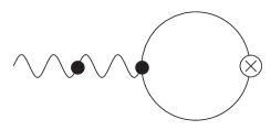
Figure 3: The breaking of fermion number symmetry upon mass generation of fermions in the $\tau_{3}$QED₃ model of [2]. The figure denotes the matrix element of the fermion number current between the vacuum and one ‘photon’ state. The dark blobs denote loop corrections and the crossed-blob denotes an insertion of the fermion number current.

Upon coupling to external electromagnetic fields $A_{\mu}$, the anomalous matrix element (2.4) (c.f. fig. 3) leads to superconductivity in the case of non compact gauge fields $a_{\mu}$, as a result of the existence of a massless pole in the electric current-current correlator [2] (c.f. fig. 4):

$$<0|J_{\mu}(k)J_{\nu}(-k)|0>=\frac{g^{2}}{\pi^{2}}\left(\frac{k_{\mu}k_{\nu}}{k^{2}}-\delta_{\mu\nu}\right)\left(1+\Pi(k)\right)^{-1}$$ (2.5)

where $\Pi(k)$ is the one-loop vacuum polarization graph.

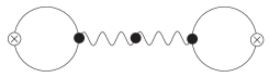
Figure 4: In non compact gauge theories the anomalous graph of fig. 3 gives rise to massless poles in the current-current correlators, as a result of the exchange of the massless statistical gauge boson $a_{\mu}$; upon coupling the system to an external electromagnetic potential, this results in superconductivity (Landau criterion).

Strictly speaking this superconducting behaviour pertains only to zero temperatures $T=0$, since at finite temperature the masslessness of the statistical gauge field $a_{\mu}$ disappears, as a result of a plasmon mass in the longitudinal component $a_{0}$. In view of the above considerations therefore, the novel $T=0$ phase predicted here would result in a modification of the temperature-doping phase diagram of high-$T_{c}$, by a quantum critical line at $T=0$, as shown in figure 5, should the $\tau_{3}$-model describe correctly the underdoped cuprate phase. It has been argued, though, in [2] that despite the plasmon longitudinal mass, the screening of the magnetic field (Meissner effect), associated with the massless transverse component of the statistical gauge field $a_{\mu}$, is still valid at finite temperatures, up to a temperature in which the nodal holon mass gap disappears. Such a temperature has been estimated in [20] to lie at most on the $mK$ scale, i.e. much lower than the optimal-doping critical temperature of $100$ K of high-temperature superconductors.

Figure 5: The anomalous graph of fig. 3 results to a novel quantum critical phase, of Kosterlitz Thouless (KT) type (no local order parameter perturbatively) strictly at $T=0$. Should the model of [2] describe the underdoped cuprate phase, then, this may modify the phase diagram of high temperature superconductors, by connecting the optimal doping superconducting phase and the antiferromagnetic phases, as indicated by the dashed line. It must be stressed, though, that if the screening of the magnetic field lines still occurs for finite temperatures up to a critical $T_{c}^{\star}$ much lower than the optimal $T_{c}\sim 100$ K of high $T_{c}$ [2], then the novel KT superconducting phase extends also inside the pseudogap phase in a region bounded by such small $T_{c}^{\star}$, as indicated by the dashed dotted line.

2.3 QED₃ in the slave-boson approach

The issue we want to bring up in this subsection is that in the non compact gauge $a$-field case, a corresponding $T=0$ anomalous behaviour characterises also the QED₃ models of [6, 5], within the slave-boson approach, but the symmetry that breaks anomalously in this case is not the fermion-number symmetry, but a version of chiral symmetry (but not the standard chiral symmetry which breaks due to the parity-conserving mass generation for fermions). In this sense, the quantum critical point does not imply superconductivity, but an anomalous behaviour within an AF phase. This quantum-critical phenomenon has been missed in the relevant recent literature [5, 6], because the analysis is restricted only to $T\neq 0$. It is our conjecture, therefore, that in QED₃ theories of the pseudogap phase of high-temperature superconductors utilizing non compact gauge fields, there is always an anomalous behaviour in the spin sector at $T=0$, which is realized via the loop graphs of figs. 3,4. By the way, we call this behaviour “anomalous” since at tree level the result is zero, and appears only at one loop.

Let us try to decipher this anomalous behaviour from studies of effective QED₃ models of the slave-boson approach to spin-charge separation developed in [5, 6]. According to the latter, the electron operators are written as:

$$c_{i,\alpha}=\xi_{i,\alpha}{\overline{b}}_{i},\quad\alpha=1,2$$ (2.6)

where $b$ are spinless bosons, carrying electric charge degrees of freedom, and represent the holons, while $\xi_{i,\alpha}$ are electrically neutral fermions, carrying spin, which represent the spinons, with $\alpha=1,2$ a spin SU(2) index. There is of course the corresponding constraint (2.2) again, expressed in terms of the new variables in (2.6).

In [5, 6] an effective continuum field theory for $\xi$ has been constructed, which yields an interacting QED₃ model of two four-component spinors $\Psi$ constructed appropriately out of $\xi_{\alpha}$, $\alpha=1,2$, interacting with a non compact statistical $U(1)$ gauge field, expressing spin frustration responsible for nodes mixing. The lagrangian reads:

$${\cal L}_{QED_{3}}=-\frac{1}{4}f^{2}_{\mu\nu}(a)+\sum_{f=1}^{2}{\overline{\tilde{\Psi}}}_{f}(i\gamma^{\mu}\partial_{\mu}+\gamma_{\mu}a^{\mu}){\tilde{\Psi}_{f}}+\dots$$ (2.7)

where ${\tilde{\Psi}_{f}}$ are electrically neutral four-component continuum spinors (spinons), and $f=1,2$ runs over node pairs as in figure 1. The massive ${\tilde{\Psi}}$ phase is characterised first of all by a breaking of (global) chiral symmetries generated by $\gamma_{5}=i\left(\begin{array}[]{rr}0&I\\ I&0\end{array}\right)$ and $\gamma_{3}=i\left(\begin{array}[]{rr}0&I\\ -I&0\end{array}\right)$, in a four-component notation for spinors with an even number of flavours, in a reducible representation of the Dirac algebra in $(2+1)$-dimensions. Above, $I$ denotes the $2\times 2$ unit matrix. These are global symmetries, whose breaking will result in the appearance of massless Goldstone bosons, to be discussed in the next section.

Figure 6: In the $QED_{3}$ model of [6, 5], the anomalous graph of fig. 3, but for the chiral symmetry breaking current ${\overline{\Psi}}{\tilde{\tau}}_{3}\gamma_{\mu}\Psi$, results to a novel quantum critical phase, of KT type (no local order parameter perturbatively) which is a spin density wave (SDW) (weak AF) phase. This novel KT superconducting phase extends inside the pseudogap phase, and covers a region from the $T=0$ line to a critical temperature which is much smaller than the critical temperature separating the pseudogap from the normal phase. For any $T\neq 0$ it becomes indistinguishable from the conventional chiral symmetry broken phase of [6], but its $T=0$ anomalous behaviour, with a massless pole in the two-point correlator of the $\tau_{3}$-chiral symmetry currents, provides a distinctive discontinuous novel behaviour. Compare/contrast the situation with that in figure 5, where one obtains an anomalous KT superconducting phase connecting the optimal doping superconducting (SC) phase with the AF phase. Here one obtains an anomalous SDW phase that connects the AF and (optimal doping) SC phases.

A dynamical mass generation (spin gap) for the spinons ${\tilde{\Psi}_{f}}$ has been argued in [5, 6] to be related with properties of the pseudogap phase of high temperature superconductors. Most importantly, the massive spinon phase has been interpreted in [6] as implying that the antiferromagnetic (AF) phase is immediately succeeded by the superconducting phase, as indicated in figure 6, in the sense of a region of weak AF (spin density wave (SDW) phase) in which the critical temperature for the new phase is much smaller than the pseudogap critical temperature. This situation is opposite to the graph in figure 5 of the model of [2], where the superconducting phase (for non compact gauge fields) enters the pseudogap region until the AF (Neel) state. The analysis of [6] did a low temperature analysis, attempting to generalize the conclusions down to the $T=0$ region. It is our purpose here to point out some important aspects of this region in QED₃, not discussed in [6], but existing in the literature [3], which like the $\tau_{3}$-QED case, imply a discontinuity of the $T=0$ line (quantum critical line).

Indeed, apart from the conventional chiral symmetry in theories with even number of fermion flavours, discussed in [6], generated by the $4\times 4$ matrix $\gamma_{3},\gamma_{5}$, there is another symmetry of (2.7)  [3, 2], whose breaking is realized in the so-called Kosterlitz-Thouless mode, without a (perturbative) local order parameter, and hence Goldstone bosons. This symmetry is generated by the ${\tilde{\tau}_{3}}=i\left(\begin{array}[]{rr}I&0\\ 0&-I\end{array}\right)$ The corresponding current generator is $J_{\mu}^{{\tilde{\tau}}_{3}}=\sum_{f=1}^{2}\overline{{\tilde{\Psi}}_{f}}{\tilde{\tau}_{3}}\gamma_{\mu}{\tilde{\Psi}_{f}}$ and, as shown in [3] its matrix element between the vacuum and the one photon state (as in fig. 3) is non-zero in the massive $\Psi$ phase:

$$<a_{\mu}|J_{\nu}^{{\tilde{\tau}_{3}}}|0>\sim\frac{{\tilde{M}}}{|{\tilde{M}}|}\epsilon_{\mu\nu\rho}\frac{p^{\rho}}{\sqrt{p_{0}}}$$ (2.8)

This also leads to $J_{\nu}^{{\tilde{\tau}_{3}}}$ current-current correlators with a massless pole for strictly a $T=0$ case, according to the corresponding graphs of fig. 4 (c.f. (2.5)). Our claim is that such a KT $T=0$ phase, with a massless pole in the respective correlator of the generating currents defines a novel quantum critical point which corresponds to an unconventional AF phase in the model of [6], or, in fact, any other QED₃ model (within the slave-boson approach) of doped AF. As in the case of $\tau_{3}$-QED, the critical temperature at which the chiral-symmetry-breaking spinon mass disappears, is also a critical temperature for this anomalous behaviour. This temperature is much smaller than the critical temperature separating the pseudogap from the normal phases in the phase diagram. The distinctive feature of this anomalous symmetry from the standard chiral symmetry, which is used in the approach of [6], is precisely its $T=0$ behaviour, where the current-current correlator for the spinon current ${\overline{\Psi}}{\tilde{\tau}}_{3}\gamma_{\mu}\Psi$ has a massless pole that disappears at any finite $T$, due to plasmon mass. This feature defines the $T=0$ as a quantum critical line, corresponding to a KT breaking of the $\tau_{3}$ chiral symmetry, defined above: we may term this phase as KT SDW (c.f. figure 6). For any $T\neq 0$ the situation is like in [6], but the $T=0$ quantum critical behaviour is distinct, and ‘discontinuous’ from the $T\neq 0$ case, and has been missed in the recent condensed matter literature [6, 5].

2.4 Compact Gauge Theories

In the above analysis the statistical gauge field had been assumed non compact. However, the spin-charge separation Ansatz might be extended to a non-Abelian form [13] by exploiting appropriately an (approximate) particle-hole symmetry of the $t-j$ Hamiltonian for underdoped cuprates:

$$\chi_{\alpha\beta,i}=\psi_{\alpha\gamma,i}z_{\gamma\beta,i}\equiv\left(\begin{array}[]{rr}c_{1}&c_{2}\\ c_{2}^{\dagger}&-c_{1}^{\dagger}\end{array}\right)_{i}=\left(\begin{array}[]{rr}\psi_{1}&\psi_{2}\\ -\psi_{2}^{\dagger}&\psi_{1}^{\dagger}\end{array}\right)_{i}~{}\left(\begin{array}[]{rr}z_{1}&-{\overline{z}}_{2}\\ z_{2}&{\overline{z}}_{1}\end{array}\right)_{i}$$ (2.9)

where the fields $z_{\alpha,i}$ obey canonical bosonic commutation relations, and are associated with the spin degrees of freedom (magnons), whilst the fields $\psi_{a,i},~{}a=1,2$ have fermionic statistics, and are assumed to create holes at the site $i$ with spin index $\alpha$ (holons). The Ansatz (2.9) has spin-electric-charge separation, since only the fields $\psi$ carry electric charge. It is a slave-fermion Ansatz since the holons are fermionic.

The Ansatz has a local SU(2) symmetry, if one defines the transformation properties of the $z$ fields to be given by left multiplication with the SU(2) matrices, and those of the $\psi^{\dagger}_{\alpha\beta}$ matrices by the left multiplication

$$\xi_{\alpha\beta}\rightarrow h_{\alpha}^{\gamma}\xi_{\gamma\beta}$$ (2.10)

In this representation, the gauge group $SU(2)$ is generated by the $2\times 2$ Pauli matrices.

The Ansatz (2.9) possesses an additional local $U_{S}(1)$ ‘statistical’ phase symmetry, which allows fractional statistics of the spin and charge excitations. This is an exclusive feature of the three dimensional geometry. This is similar in spirit, although implemented in an admittedly less rigorous way, to the bosonization technique of the spin-charge separation Ansatz of ref. [9], and allows the alternative possibility of representing the holes as slave bosons and the spin excitations as fermions.

In addition, as a consequence of the fact that the fermions $\psi$ carry electric charge, one has an extra $U_{em}(1)$ symmetry for the problem.

To recapitulate, the above analysis, based on the spin-charge separation Ansatz (2.9) which allows spin flip, leads to the following local-phase (gauge) group structure for the doped large-$U$ Hubbard model:

$$G=SU(2)\otimes U_{S}(1)\otimes U_{em}(1)$$ (2.11)

where the second $U_{em}(1)$ factor refers to electromagnetic symmetry due to the electric charge of the holes. This symmetry appears as a hidden symmetry of the effective holon and spinon degrees of freedom obeying the Ansatz (2.9).

The statistics-changing $U_{S}(1)$ group is strongly coupled, given that in the resulting effective lagrangian appears without a Maxwell Kinetic term, and hence it may be considered of (formally) infinitely string coupling $g_{s}\rightarrow\infty$. In practice, the coupling is cutoff by an effective cutoff which may be defined by the highest scale in the problem (e.g. the strong Hubbard coupling $U$ in Hubbard models with a strong repulsion $U\gg 1$ so as to implement the one-electron per site constraint, or the Heisenberg interaction $J$ in $t-J$ models [13]). Such strong Abelian groups may be responsible for dynamical mass generation of fermions (holons).

The effective continuum theory obtained from (2.9) around the nodes of the underdoped cuprates consists of Dirac spinors, representing the holons, as well as $z$ magnons, interacting via the non-Abelian gauge interactions. The holons are coupled to the full Non-Abelian group G, while the $z$ magnons, being electrically neutral, couple only to the $SU(2)\otimes U_{S}(1)$ subgroup.

The dynamically generated mass for the holons is parity conserving as a result of the vector-like nature of the interactions in the simplest model considered [19]. As discussed in detail in [13], such parity-conserving mass term break dynamically the SU(2) subgroup, due to the fact that the parity conserving mass term for fermions transform like triplets under this SU(2).

As a result of the breaking $SU(2)\rightarrow U_{c}(1)$, two of the gauge bosons of SU(2) acquire heavy masses, and decouple from the effective low-energy theory. One is then left with an effective theory of massless degrees of freedom consisting of the unbroken subgroup associated with the $\tau_{3}=\left(\begin{array}[]{rr}1&0\\ 0&-1\end{array}\right)$ generator of the SU(2) group. This model is then nothing else but the $\tau_{3}$ QED model of [2], discussed above, with the important difference that now the statistical unbroken gauge group $U_{c}(1)$ is compact.

Compact groups are known to have non-perturbative monopole configurations , which in (2+1)-dimensions are like instantons, having a point-like structure. Such monopole instantons are responsible in general for the generation of a small non-perturbative mass of the statistical photons of the $U_{c}(1)$ group [21]:

$${\rm photon~{}mass}\equiv m_{\gamma}\sim e^{-2S_{0}}$$ (2.12)

where the above computations have been performed in a dilute instanton gas, $S_{0}$ is the one-instanton action, and the factor of $2$ in the exponent is due to the fact that the theory has fermions [23]. The presence of a non-perturbative photon mass, implies that in the compact case there is no longer a massless pole in the electric current-current correlator (2.5). As a consequence, the KT $T=0$ superconducting quantum-critical line of the non-compact case is absent, and the AF phase is separated by the (optimal doping) superconducting one in the phase diagram of fig. 5 by a pseudogap phase, which in this case extends all the way down to $T=0$.

3 Counting degrees of freedom: a tricky business

We would now like to address the issue of dynamical generation of the fermion mass per se in all the above cases, (A) and (B). As we have discussed, such a mass generation is crucial for the existence of the novel quantum-critical ‘anomalous’ phases. To this end, in this section we shall briefly review first the non perturbative arguments of [10], according to which dynamical mass generation can only occur in a theory with $N_{f}$ four-component spinors, with $N_{f}\leq N_{c}=3/2$, showing that the previous large-$N$ treatment [18] overestimated $N_{c}$. If this result were true in our case, this would mean that the above-described QED₃ model [6, 5], with two four-component spinors (spinons) constructed as in fig. 1, would never have a quantum phase with broken ${\tilde{\tau}_{3}}$ symmetry, since the spinons would be massless. However, as we shall discuss below, the arguments of [10] may not go through in (2+1)-dimensions for a variety of reasons. At this stage we would like to mention, however, that even if such arguments were assumed to be valid in (2+1)-dimensional gauge theories, nevertheless their application to the $\tau_{3}$-QED model [2] does not select a critical number for mass generation of the electrically charged fermions, leaving this task to a detailed SD analysis or other studies. Below we shall explain in detail why this is so, but we will also provide arguments supporting the point of view that the analysis of [10] are not applicable to the (2+1)-dimensional QED₃ model either.

We commence our discussion by first going over the new proposed constraint on strongly coupled field theories. of [10] The constraint was based on a counting of massless degrees of freedom between IR and UV fixed points, leading to inequalities between the respective values of the renormalized free energy density. This resembles, but is not identical to, the celebrated C-theorem of Zamolodchikov for two-dimensional conformal field theories [24]. The conjectured constraint of [10], has not been proven; nevertheless, its validity has been verified in a number of physically relevant examples. The conjecture of [10] implies a reduction in the massless degrees of freedom as the theory flows under Renormalization Group (RG) from UV to IR fixed points. In what follows we shall therefore examine the applicability of the conditions leading to the constraint for the above-described QED₃-like models of potential interest to the physics of doped antiferromagnets.

For instructive purposes, let us first state the form of the constraint of ref. [10] and the main assumptions leading to it: The main thrust of the constraint is associated with an inequality between the values of an extensive quantity, such as the free energy, at the UV and IR fixed points of asymptotically free field theories. Specifically, it has been argued that the quantity $f_{\rm UV}=-{\rm lim}_{T\rightarrow\infty}\frac{{\cal F}}{T^{4}}\frac{90}{\pi^{2}}$ where ${\cal F}$ is the free energy of the system, and $T$ is the temperature, playing here the rôle of a varying RG scale in the problem, counts the massless degrees of freedom in the UV, while a similar quantity: $f_{\rm IR}=-{\rm lim}_{T\rightarrow 0}\frac{{\cal F}}{T^{4}}\frac{90}{\pi^{2}}$ counts the massless IR degrees of freedom of the system. The conjectured inequality states that:

$$f_{\rm IR}\leq f_{\rm UV}$$ (3.1)

An important ingredient for the validity of Eq. (3.1) is the asymptotic freedom of the theory in question. In fact, there are known examples that do not satisfy the inequality if they exhibit a non-trivial UV fixed point [10].

The inequality (3.1) has been applied to QED₃, which is known to exhibit chiral symmetry breaking in the IR. The theory has a dimensionfull coupling, and in [10], it has been assumed free in the UV. According to [10], this implies the following contributions of massless degrees of freedom to $f_{\rm UV}$ (in three space time dimensions): one from the massless photon in (2+1)-dimensions, and $(3/4)~{}4N$ from $N$ four-component free fermions. Hence one has at the UV:

$$f_{\rm UV}=1+3N$$ (3.2)

On the other hand, in the IR, there is a dynamical generation of fermion masses, which implies a breaking of the global chiral symmetry of the massless theory $U(2N)\rightarrow U(N)\times U(N)$. In this case there are 2N² massless Goldstone bosons. The authors of [10] deal with non compact QED₃, and hence the photon remains massless in the IR, which implies the following contribution to $f_{\rm IR}$ :

$$f_{\rm IR}=1+2N^{2}$$ (3.3)

From the inequality (3.1), and (3.2), (3.3), then, one obtains a critical number of fermion flavours for chiral symmetry breaking to take place; in particular $N<N_{c}=3/2$, a result, which, if true, would imply that the early papers on dynamical mass generation [18] overestimated the critical number, placing it in the region $3<N_{c}<4$.

Now let us go over these assumptions one by one:

• (1) Asymptotic freedom: In the context of perturbation theory QED₃ is super-renormalizable (i.e. it contains a finite number of divergent diagrams); this is a direct consequence of simple power-counting, given that the dimensionfull gauge coupling scales as $[M]^{1/2}$. However, QED₃ is not asymptotically free, in the same way that the super-renormalizable $(\phi^{3})_{4}$ is not (this latter theory has a dimensionfull coupling as well): the coupling does not go to zero for large momenta $p\rightarrow\infty$. In fact, strictly speaking, the coupling does not display any energy dependence at all, because the corresponding $\beta$ function vanishes, i.e. $\beta_{QED_{3}}\equiv\mu\left(de/d\mu\right)=0$. This is true simply because the vacuum polarization in $d=3$ is finite, and thus no wave-function renormalization for the photon is needed. The above renormalization group equation simply states that $e=e_{0}$, where $e_{0}$ is the initial tree-level coupling. Clearly such a theory cannot be asymptotically free (at least in a perturbative context), unless $e_{0}=0$; but then this would imply that the theory is non-interactive (i.e. trivial) throughout. This situation is to be contrasted to what happens in the case of a bona fide asymptotically free theory, such as QCD₄. In this case $\beta_{QCD_{4}}=-b_{0}g^{3}$ ($b_{0}>0)$; when solving this equation one obtains the usual logarithmic dependence of the coupling $g$ on $p$, which, in the limit $p\rightarrow\infty$, leads to an asymptotically non-interactive theory (i.e. the value of the coupling goes to zero, not just to some constant value).

  Given the discussion above, in order to obtain some sort of non-trivial structure in the UV, one must study QED₃ outside the realm of standard perturbation theory. In particular, arguments supporting asymptotic freedom of QED₃, and hence the counting in the UV leading to (3.2), are based on large $N$ treatments. Indeed, in such an approximation [25] one defines a dimensionless effective running number of flavours, which turns out to scale with the momenta as (in the non-local gauge):

  $${\rm(effective~{}coupling)^{2}/scale}=\frac{1}{N_{\rm run}(p)}\sim\frac{1}{1+\frac{g_{0}}{3}{\rm ln}p/\alpha}~{};~{}g_{0}\equiv\frac{8}{\pi^{2}}$$ (3.4)

  An obvious drawback of the large $N$ treatment in this context is the fact that, even though the expansion is in principle systematic due to the presence of a parameter ($N$) which may be formally taken to infinity, in practice the desired effects are obtained by stretching the validity of this approximation into a range of $N$ values which one might consider as “uncomfortably small”. In particular, an upper bound on the critical number of flavours $N<N_{c}\sim 3/2$ is obtained, beyond which chiral symmetry breaking is not possible. In this scheme the fundamental photon-fermion vertex is assumed to have the form $\Gamma_{\mu}=\gamma_{\mu}A^{n}(p)$, where $A(p)$ is the wave function renormalization. For the case $N=2$ there is no running and the model is not asymptotically free. For $N>2$ the theory is asymptotically free, while for $N<2$ the theory behaves like QED₄ with a Landau pole.

  

  Figure 7: The dotted line represents the constant (non-running) coupling obtained from the $\beta_{QED_{3}}=0$ condition, and the solid line is the running obtained through the effective charge of Eq.(3.10). In both cases the theory is not asymptotically free, because the coupling saturates at a non-zero value. For comparison, the $QCD_{4}$ coupling (perforated line) approaches asymptotically the value zero (asymptotic freedom)

  The Effective charge:

  Given that, due to the super-renormalizability of QED₃ one obtains no standard running for the coupling, one might be tempted to explore other field-theoretic alternatives. In particular one may ask what sort of “running” one obtains from the “effective charge” in the case at hand.

  In QED₄ the infinite subset of radiative corrections summed in the Dyson series generated by the one–particle–irreducible vacuum polarization $\Pi_{R}(p^{2})$ defines an effective charge which is gauge–, scale–, and scheme–independent to all orders in perturbation theory:

  $$e^{2}_{\rm eff}(p^{2})=\frac{e_{R}^{2}}{1+\Pi_{R}(p^{2})}=\,\frac{e^{2}}{1+\Pi(p^{2})}\,,$$ (3.5)

  where we have used $e_{R}^{2}=(Z_{2}^{2}Z_{3}/Z_{1}^{2})e^{2}$ and $1+\Pi_{R}=Z_{3}(1+\Pi)$ together with the QED Ward identity $Z_{1}=Z_{2}$ to write $e^{2}_{\rm eff}(q^{2})$ purely in terms of bare quantities. At $p^{2}/m_{f}^{2}\rightarrow\infty$, the effective charge $e^{2}_{\rm eff}(p^{2})$ matches on to the running coupling $\bar{e}^{2}(p^{2})$ defined from the renormalization group: at the one–loop level,

  $$\lim_{p^{2}/m_{f}^{2}\rightarrow\infty}e^{2}_{\rm eff}(p^{2})=\bar{e}^{2}(p^{2})=\frac{e^{2}_{R}}{1-\frac{e^{2}_{R}}{12\pi^{2}}n_{f}\log(p^{2}/m_{f}^{2})}\,,$$ (3.6)

  where $n_{f}$ is the number of fermion flavors. What makes the effective charge a particularly useful concept is its non-trivial dependence on masses, through the analyticity properties of $\Pi(p^{2})$. In particular, when $p^{2}>4m_{0}^{2}$ the vacuum polarization has imaginary part $\Im m\Pi(p^{2})$ given by

  $$\Im m\Pi(p^{2})=\vartheta(p^{2}-4m_{0}^{2})\frac{\alpha}{3}\Bigg{(}1+\frac{2m_{0}^{2}}{p^{2}}\Bigg{)}\sqrt{1-\frac{4m_{0}^{2}}{p^{2}}}\,,$$ (3.7)

  By virtue of analyticity the real part $\Re e\Pi(p^{2})$ may be reproduced from $\Im m\Pi(p^{2})$ by means of a once–subtracted dispersion relation Thus, for the one–loop contribution of the fermion $f$, choosing the on–shell renormalization scheme,

  $$\Re e\Pi(p^{2})=\bigg{(}\frac{1}{\pi}\bigg{)}p^{2}\,\int_{4m_{0}^{2}}^{\infty}ds\frac{\Im m\Pi(s)}{s(s-p^{2})}$$ (3.8)

  Finally, the one-loop $\Im m\Pi(p^{2})$ is directly related, via the optical theorem, to the tree level cross sections for the physical processes $e^{+}e^{-}\rightarrow f^{+}f^{-}$, with $f\neq e$,

  $$\Im m\Pi(s)=\frac{s}{4\pi\alpha}\,\sigma(e^{+}e^{-}\rightarrow f^{+}f^{-})$$ (3.9)

  The aforementioned properties of the 4-$d$ effective charge go through in the case of QED₃, with the appropriate adjustments due to the fact that no renormalization is needed (for example, the 3-$d$ analogue of the dispersion relation in Eq.(3.8) needs no subtraction). In the case of QED₃ the dimensionless effective charge reads

  $$e^{2}_{\rm eff}(p)/\alpha=\frac{1}{1+\Pi(p^{2})}$$ (3.10)

  where $\Pi(p^{2})$ is the scalar co-factor of the one-loop vacuum polarization $\Pi_{\mu\nu}(p)=(p^{2}g_{\mu\nu}-p_{\mu}p_{\nu})\Pi(p^{2})$ in $d=3$; in particular, $\Pi(p^{2})=-\alpha/8p$. The qualitative behavior of $e_{\rm eff}(p)$ is shown in fig.(7), solid line: For large $p$ the effective charge saturates to a non-vanishing value $e_{0}$, i.e. it does not display asymptotic freedom.

• (2) IR infinities and the Mermin-Wagner theorem:

  The argument leading to the inequality (3.1) is based on a finite temperature extension. However, in two spatial dimensions at finite temperature there are IR infinities as $T\rightarrow 0$, which invalidate the well-defined nature of Goldstone bosons. Such IR infinities can be seen in the effective IR cut-off dependence of the running flavour number at any finite temperature $N=N({\rm ln}T)$ which stems from solving large-$N$ SD equations in the presence of an IR cutoff [25, 29, 30]. One may question the robustness of large-$N$ treatments, but the presence of IR infinities is probably indisputable.

  The absence of Goldstone bosons, due to IR infinities (Mermin-Wagner theorem), implies the following counting of massless degrees of freedom in the IR: $f_{\rm IR}=1$. Hence in that case the inequality (3.1) becomes formally (even assuming asymptotic freedom):

  $$f_{\rm IR}=1<f_{\rm UV}=1+3N\quad\rightarrow N>1/3$$ (3.11)

  hence we obtain no non-trivial information from this constraint. In fact the above counting is formal, given that the IR infinities imply ln$T$ divergences as $T\rightarrow 0$ in the effective action, and hence in $f_{\rm IR}$. One therefore has to do the computation explicitly to regularize these divergences [30, 29], which leads to IR-cutoff- (and hence temperature-) dependent critical number of fermion flavours $N_{c}(T)$.

• (3) This and the following items are physical reasons why the inequality (3.1) does not apply to systems of interest in our case.

  In most theories of condensed matter for high temperature superconductors there are four fermion interactions present, in addition to the gauge minimal coupling terms. It is well known that [17] four-Fermi theories in less than four dimensions are renormalizable (in a large $N$ treatment at least), and they exhibit a non-trivial UV fixed point. This is sufficient to invalidate the counting of degrees of freedom leading to $f_{\rm UV}$ (3.2) in this case, and hence the inequality (3.1) for such systems.

• (4) Another important physical system which may imply a different critical number even if one accepts the inequality (3.1) is the model for high temperature superconductivity of [2] known as $\tau_{3}$QED₃, whose lagrangian is given in (2.3). The important difference of this model from QED₃ (2.7) lies in the original global symmetries. Namely, in the $\tau_{3}$QED model (2.3), due to the opposite couplings of the two fermionic ‘colors’ (each color is a four component spinor), the symmetry that is broken is a global fermion number symmetry $J_{\mu}={\overline{\psi}}_{c,f}\gamma_{\mu}\psi_{c,f}$ . As discussed previously the symmetry is broken through the anomaly graph of figure 3. The figure denotes the S-matrix element

  $$<a_{\mu}|J_{\nu}|0>={\rm sgn}(m)\epsilon_{\mu\nu\rho}p_{\rho}/\sqrt{p_{0}}$$ (3.12)

  (where $p_{0}$ is the energy) in the phase where there is mass generation $m$ for the fermions. From the breaking of the global $U(1)$ symmetry there is one Goldstone boson but again there is no local order parameter. In that case the counting of the inequality (3.1) implies $1+3N>2$ i.e. $N>1/3$. Note that in this model, if one applies the Mermin-Wagner theorem, according to which there is no well defined Goldstone boson, then the above inequality would only imply $N\geq 0$. At any rate, the coupling of the system to electromagnetism, promotes the global fermion number $U(1)$ symmetry to a local electromagnetic symmetry, whose breaking results in superconductivity. In that case the would-be Goldstone boson is eaten by the longitudinal component of the electromagnetic potential, which now acquires a mass [2].

This completes our discussion on the limitations of the applicability of the constraints of ref. [10] on the three-dimensional gauge systems of interest to us here. In the next section we proceed to review a SD analysis, which sheds some light on the non-asymptotic freedom of the effective QED₃ model, the absence of a critical number of fermion flavours for chiral symmetry breaking, but the existence of a region of the effective charge where the phenomenon takes place. In addition we also discuss the non-trivial IR fixed point structure of QED₃. We believe that all these features are physically important; especially the last one implies the non-Fermi liquid behaviour of the relativistic spin liquid of nodal excitations under consideration.

4 SD equations and Critical Number of Flavours

In this section we will present a study of the issue of mass generation and chiral symmetry breaking in the framework of the SD equations.

Figure 8: The Schwinger-Dyson (SD) equations for the photon and fermion self energies, and the vertex function. The blobs indicate the full (non-perturbative) corrections.

The derivation of the SD equations for the photon propagator $\Delta_{\mu\nu}$, the electron propagator $S_{F}$, and the photon-electron vertex $\Gamma_{\mu}$ in QED₃ proceeds following standard methods [31, 32]. The result is schematically depicted in fig. 8:

$$\Delta_{\mu\nu}^{-1}(q) = \Delta^{-1}_{0\mu\nu}(q)+e^{2}\int\frac{d^{3}k}{(2\pi)^{3}}{\rm Tr}[\Gamma_{\mu}S_{F}\Gamma_{\nu}S_{F}]~{}+\dots$$

$$S_{F}^{-1}(p) = {S_{0F}^{-1}}(p)-e^{2}\int\frac{d^{3}k}{(2\pi)^{3}}\Gamma_{\mu}S_{F}\Gamma_{\nu}\Delta^{\mu\nu}~{}+\dots$$ (4.1)

$$\Gamma_{\mu}(p_{1},p_{2},p_{3}) = \gamma_{\mu}-e^{2}\int\frac{d^{3}k}{(2\pi)^{3}}\Gamma_{\alpha}S_{F}\Gamma_{\mu}S_{F}\Gamma_{\beta}\Delta^{\alpha\beta}+\dots$$

where $\Delta^{-1}_{0\mu\nu}(q)=q^{2}g_{\mu\nu}+(\xi^{-1}-1)q_{\mu}q_{\nu}$, ${S_{0F}^{-1}}(p)=/p-m$, and $p_{1}+p_{2}+p_{3}=0$. The ellipses on the right-hand sides denote the infinite set of terms containing the two-particle irreducible four-point function [31, 32]. Although we are not working in the context of a large-$N$ analysis, we note that the above truncation is compatible with working to leading order in resummed $1/N$ expansion.

We next define the scalar quantities $A$, $B$ and ${\cal G}$ as follows:

$$S_{F}(k)=\frac{1}{A(k)~{}/k},\,\,\,\,\,\,\,\Delta_{\mu\nu}(k)=\frac{g_{\mu\nu}}{B(k)k^{2}},\,\,\,\,\,\,\,\Gamma_{\mu}(p_{1},p_{2},p_{3})={\cal G}(p_{1},p_{2},p_{3})\gamma_{\mu}$$ (4.2)

Note that the form of Eq.(4.2) implies that the longitudinal pieces of the photon propagator will be discarded in what follows; this is motivated by the PT analysis presented in the Appendix, particularly points (iv) and (v) of the last subsection.

4.1 The semi-amputated vertex

Following [12] and [33] we define the semi-amputated vertex ${\hat{G}}$ as

$${\hat{G}}(p_{1},p_{2},p_{3})\equiv Z(p_{1},p_{2},p_{3}){\cal G}(p_{1},p_{2},p_{3})$$ (4.3)

with

$$Z(p_{1},p_{2},p_{3})=B^{-1/2}(p_{1})A^{-1/2}(p_{2})A^{-1/2}(p_{3})$$ (4.4)

This definition proves very useful in reducing the complexity of the set of SD equations. In addition, as explained in [34] the quantity

$$g_{R}(p_{1},p_{2},p_{3})\equiv e{\hat{G}}(p_{1},p_{2},p_{3})$$ (4.5)

provides a natural generalisation of the concept of the running or “effective” charge in the context of super-renormalizable gauge theories, such as QED₃.

The equation for the semi-amputated vertex $\hat{G}$ may be obtained from the third equation in (4) by multiplying both sides by the factor $Z(p_{1},p_{2},p_{3})$, i.e.

$${\hat{G}}(p_{1},p_{2},p_{3})\gamma_{\mu}=Z(p_{1},p_{2},p_{3})\gamma_{\mu}-e^{2}\int\frac{d^{3}k}{(2\pi)^{3}}{\hat{G}}^{3}\gamma^{\alpha}\frac{1}{/k-/p_{1}}\gamma_{\mu}\frac{1}{/k}\gamma_{\alpha}\frac{1}{(k+p_{2})^{2}}$$ (4.6)

where ${\hat{G}}^{3}\equiv{\hat{G}}(p_{3},k+p_{2},p_{1}-k){\hat{G}}(p_{1},-k,k-p_{1}){\hat{G}}(p_{2},k,-k-p_{2})$. Restricting ourselves to the case where the photon momentum is vanishingly small, one is left with a single momentum scale $p$. One can then define a renormalization-group $\beta$ function from this “running” coupling $G(p)$ by setting $\beta\equiv p\bigg{(}d{\hat{G}}(p)/dp\bigg{)}$. In order to further simplify the SD equation for $G(p)$ we make the additional approximation that ${\hat{G}}^{3}={\hat{G}}^{3}(k)$, i.e. a cubic power of a single ${\hat{G}}(k)$ depending only on the integration variable $k$.

Carrying out the $\gamma$-matrix algebra in $d=3$-dimensional Euclidean space, one obtains:

$${\hat{G}}(p)=Z(p)+\frac{1}{3}e^{2}\int\frac{d^{3}k}{(2\pi)^{3}}{\hat{G}}^{3}(k)\frac{1}{k^{2}(k-p)^{2}}$$ (4.7)

We observe that $Z(p)\rightarrow 1$ for $p\rightarrow\infty$, where perturbation theory is valid. This is expected from the fact that in such a case the functions $A(p),B(p)\rightarrow 1$ trivially. Moreover, from (4.7) we see that, if ${\hat{G}}$ stays positive, which is expected for any physical theory, then, as a result of the positivity of the integrand, $G(p)\geq 1$ for any $p$. Thus, one has the following basic properties of ${\hat{G}}(p)$, which stem directly from the integral equation (4.7): ${\hat{G}}(p)\geq 1$, (for all  $p$), and ${\hat{G}}(p)\rightarrow 1,\quad p\rightarrow\infty$. Assuming that in the IR regime, $k/\alpha<<1$, the inhomogeneous term $Z(p)$ goes to zero, (this assumption has been justified by explicit calculations in [34]) one can decouple the equation for the amputated vertex from the equations for $A(p)$, $B(p)$. Thus, one arrives at the homogeneous integral equation

$${\hat{G}}(p)=\frac{1}{3}e^{2}\int\frac{d^{3}k}{(2\pi)^{3}}{\hat{G}}^{3}(k)\frac{1}{k^{2}(k-p)^{2}}$$ (4.8)

involving only one unknown function, namely ${\hat{G}}$, which must be self-consistently determined. Note that Eq.(4.8)is invariant under the rescaling ${\hat{G}}\rightarrow{\hat{G}}/e$. This indicates a straightforward extension of the analysis to a large-$N$ treatment, given that $N$ appears only as a multiplicative factor. Eq.(4.8) does not admit physically acceptable solutions, i.e. solutions with ${\hat{G}}\geq 0$ and finite. Indeed, setting $p=0$ one obtains after the (trivial) angular integration

$${\hat{G}}(0)=\frac{e^{2}}{12\pi^{2}}\int_{0}^{\infty}\frac{dk}{k^{2}}{\hat{G}}^{3}(k)$$ (4.9)

Finiteness of ${\hat{G}}(0)$ requires that the integrand of the right hand side of (4.9) converges at $y\rightarrow 0~{}{\rm and}~{}\infty$. The UV limit does not present a problem, because the kernel vanishes like $y^{-2}$, which is consistent with the super-renormalizability of the theory as well as the fact that the amputated vertex tends to 1. In the IR limit $y\rightarrow 0$, however, the kernel blows up. For the integral to remain finite at that point, as required by the finiteness assumption for ${\hat{G}}(0)$, $G^{3}(y)$ must approach zero as $y^{\alpha},~{}\alpha>1/3$, thereby implying that ${\hat{G}}(0)=0$. However for that to happen the integrand in (4.9) must change sign, which would in turn imply that ${\hat{G}}(y)$ itself must change sign somewhere in $y$. According to our assumption above this is not a physically acceptable situation.

The way to see that indeed the behaviour $G(y)\sim y^{1/2}$ as $y\rightarrow 0$, would be the only possibility is to convert the integral equation into a non-linear differential equation. To this end, we perform the angular integration in (4.8), to arrive at the equation:

$${\hat{G}}(p)=\frac{2}{3\pi^{2}}\frac{\alpha}{p}\int_{0}^{\infty}\frac{dk}{k}{\hat{G}}^{3}(k){\rm ln}|\frac{k+p}{k-p}|$$ (4.10)

where we have set $e^{2}\equiv 8\alpha$ to make contact with the usual large-$N$ definition [18]. For us, however, the number of fermion flavours is not assumed to be necessarily large. Introducing the dimensionless variables $x\equiv p/\alpha$ and $y\equiv k/\alpha$, one obtains in the limit $x<<1$

$${\hat{G}}(x)=\frac{2}{3\pi^{2}x}\int_{0}^{\infty}\frac{dy}{y}{\hat{G}}^{3}(y){\rm ln}|\frac{y+x}{y-x}|\simeq\frac{4}{3\pi^{2}}\Bigg{(}\frac{1}{x^{2}}\int_{0}^{x}dy{\hat{G}}^{3}(y)+\int_{x}^{\infty}\frac{dy}{y^{2}}{\hat{G}}^{3}(y)\Bigg{)}$$ (4.11)

Differentiating appropriately with respect to $x$, and conveniently rescaling ${\hat{G}}$ by setting $G\equiv\sqrt{\frac{8}{3\pi^{2}}}{\hat{G}}$, we arrive at the following differential equation for small $x$:

$$x^{3}\frac{d^{2}G}{dx^{2}}+3x^{2}\frac{dG}{dx}+G^{3}(x)=0,\qquad x<<1$$ (4.12)

The obvious solution of this equation, for $x<<1$, is $G(x)=\frac{\sqrt{5}}{2}x^{1/2}$. Note that this solution would imply a ‘trivial IR fixed point structure’ given that its associated $\beta$ function vanishes at $x=0$. As we shall demonstrate below this is in fact the only solution with $G\geq 0$. Indeed, upon the change of variables $\xi^{-1}=2x^{2}$, $G=2^{3/4}~{}\eta(\xi)$, the equation becomes of Emden-Fowler type [35, 36]:

$$\frac{d^{2}}{d\xi^{2}}\eta(\xi)-\xi^{-3/2}\eta^{3}(\xi)=0,\qquad\xi\rightarrow+\infty$$ (4.13)

As discussed in the mathematical literature [35], the only positive solution of (4.13), as $\xi\rightarrow+\infty$, has the form as $\xi\rightarrow+\infty$:

$$\eta(\xi)=\frac{\sqrt{5}}{4}\xi^{-1/4},\qquad$$ (4.14)

which is exactly the solution $G(x)=\frac{\sqrt{5}}{2}x^{1/2}$ found above, in the region $x\rightarrow 0$.

The above analysis suggests that no non-trivial IR-fixed point is possible in QED₃ in the absence of an IR cut-off, as already conjectured in ref. [29].

4.2 The IR fixed point

We next study the behaviour of the SD equation for ${\hat{G}}(p)$ in the presence of an IR cut-off. W shall consider the case of a fermion mass gap $m(p)=\Sigma(p)/A(p)$, where $\Sigma(p)$ is the fermion self energy. In that case the fermion propagator $S_{F}^{-1}$ becomes:

$$S_{F}(k)=\frac{1}{A(k)\left(/k+m_{f}(k)\right)}$$ (4.15)

and we assume that $m_{f}(p)\simeq m_{f}(0)\equiv m_{f}\neq 0$. In that case the integral equation (4.8) becomes:

$${\hat{G}}(p)=\frac{e^{2}}{3}\Bigg{(}\int\frac{d^{3}k}{(2\pi)^{3}}\frac{{\hat{G}}^{3}(k)}{(k^{2}+m_{f}^{2})(k-p)^{2}}+2m_{f}^{2}\int\frac{d^{3}k}{(2\pi)^{3}}\frac{{\hat{G}}^{3}(k)}{(k^{2}+m_{f}^{2})^{2}(k-p)^{2}}\Bigg{)}$$ (4.16)

Performing the angular integrations one arrives at:

$${\hat{G}}(x)=\frac{2}{3\pi^{2}x}\int dyf(y){\rm ln}\left|\frac{y+x}{y-x}\right|{\hat{G}}^{3}(y)$$ (4.17)

where $x\equiv p/\alpha$, $m\equiv m_{f}/\alpha$ are dimensionless, and

$$f(y)\equiv y\frac{y^{2}+3m^{2}}{(y^{2}+m^{2})^{2}}\geq 0$$ (4.18)

Differentiation with respect to $x$ yields:

$$x\frac{d}{dx}{\hat{G}}(x)=-\frac{2}{3\pi^{2}x}\int_{0}^{\infty}dyf(y)\left({\rm ln}\left|\frac{y+x}{y-x}\right|+\frac{2xy}{x^{2}-y^{2}}\right){\hat{G}}^{3}(y)$$ (4.19)

One observes that formally as $x\rightarrow 0$ the right-hand-side vanishes, provided that ${\hat{G}}$ is finite. This indicates the existence of a fixed point. As we shall show below this is confirmed analytically by converting the integral equation into a non-linear differential equation. To accomplish this, one expands the logarithms for small $x<<1$, and then differentiates with respect to $x$, arriving at

$$x(x^{2}+m^{2})^{2}\frac{d^{2}}{dx^{2}}{\hat{G}}(x)+3(x^{2}+m^{2})^{2}\frac{d}{dx}{\hat{G}}(x)+\frac{8}{3\pi^{2}}(x^{2}+3m^{2}){\hat{G}}^{3}(x)=0$$ (4.20)

In the IR region $x<<m$ the equation (4.20) is approximated by:

$$x\frac{d^{2}}{dx^{2}}{\hat{G}}(x)+3\frac{d}{dx}{\hat{G}}(x)+\frac{8}{\pi^{2}m^{2}}{\hat{G}}^{3}(x)=0$$ (4.21)

and is immediate to see that a special power-law solution is given by (for positive $G(x)$) by:

$${\hat{G}}(x)=m\pi\frac{\sqrt{3}}{4\sqrt{2}}x^{-1/2}$$ (4.22)

Notice the IR divergence of this type of solutions even in the presence of a (bare) fermion mass. The associated renormalization-group $\beta$ function for this case reads:

$$\beta(x)=-\frac{1}{2}{\hat{G}}\sim x^{-1/2}\rightarrow+\infty,~{}{\rm as}~{}x\rightarrow 0$$ (4.23)

indicating the absence of an IR fixed point. The associated operator appears to be relevant (negative scaling dimension), which implies the possibility of the theory driven to a non-trivial fixed point.

However, in the IR regime $x<<1$, one can find a different type of solution:

$${\hat{G}}=m\pi\frac{\sqrt{3}}{2\sqrt{2}}\frac{c}{1+c^{2}x},\qquad x\rightarrow 0$$ (4.24)

where $c$ is a constant of integration to be fixed by the boundary condition at $x=0$ implied by the integral equation, to be discussed later on. For physical solutions $c$ is assumed positive. This type of solutions has a renormalization-group $\beta$-function of the form:

$$\beta=-{\hat{G}}(x)+\frac{2\sqrt{2}}{\sqrt{3}\pi mc}{\hat{G}}^{2}(x)\sim-\frac{x}{\left(1+c^{2}x\right)^{2}}\rightarrow 0,\qquad x\rightarrow 0$$ (4.25)

from which we observe the existence of a non-trivial (non-perturbative) IR fixed point at ${\hat{G}}^{*}=\frac{\pi m\sqrt{3}c}{2\sqrt{2}}>0$. Such a fixed point is the result of the dynamical generation of a parity-invariant, chiral-symmetry breaking fermion mass [18], indicating the connection of the phenomenon of chiral symmetry breaking in QED₃ with a non-trivial IR fixed point structure.

The non-trivial fixed-point solution (4.24) is compatible with the integral equation (4.16) for some values of the fermion mass $m$ to be specified below. Indeed, one can derive a boundary condition for ${\hat{G}}(0)$ from (4.16), which reads:

$${\hat{G}}(0)=\frac{4}{3\pi^{2}}\int_{0}^{\infty}dy\frac{{\hat{G}}^{3}(y)}{y^{2}+m^{2}}+\frac{8m^{2}}{3\pi^{2}}\int_{0}^{\infty}dy\frac{{\hat{G}}^{3}(y)}{(y^{2}+m^{2})^{2}}$$ (4.26)

In contrast to the massless case (4.9), ${\hat{G}}(0)$ is now a finite constant, $\pi mc\sqrt{3/8}$, as seen from (4.24), and this allows for a compatibility of the solution (4.24) with (4.26), provided that $m{\hat{G}}(0)$ satisfies certain conditions. Such conditions have been derived in [34], where a full analysis of the non linear coupled system of vertex, fermion and photon self-energy integral equations has been performed. The result is summarized in the equation:

$$m<\frac{\frac{8}{3\pi}\left(1-\frac{1}{\pi}\right)}{{\hat{G}}(0)-\frac{12\sqrt{6}}{5}},\qquad{\hat{G}}(0)>\frac{12\sqrt{6}}{5}\simeq 5.88~{}.$$ (4.27)

This condition will act as a boundary condition for the allowed values of $m$ in a mass-coupling diagram, as we shall discuss later on.

4.3 Dynamical generation of the fermion mass gap

In the previous subsection we have assumed the presence of a finite fermion mass, which we have treated effectively as an arbitrary parameter of the model. In this subsection we turn to the full problem, and study the dynamical generation of this mass, by deriving it self-consistently from the corresponding SD mass-gap equation.

The equation for the gap $\Sigma(p)$ reads

$$A(p)~{}/p+\Sigma(p)=/p+A(p)e^{2}\int\frac{d^{3}k}{(2\pi)^{3}}{\hat{G}}^{2}(k)\gamma_{\mu}\frac{1}{/k+M(k)}\gamma^{\mu}\frac{1}{(k-p)^{2}}$$ (4.28)

where $M(k)\equiv\Sigma(k)/A(k)$ is the mass function, and we have pulled out factors of $A(p)$ appropriately so as to be able to define an amputated vertex function ${\cal G}(k)$. After standard algebraic manipulations, using dimensionless variables, in units of $\alpha=e^{2}/8$, ${\tilde{M}}\equiv M(k)/\alpha$, $x\equiv p/\alpha$, $y\equiv k/\alpha$, and working in the regime of low momenta $x<<1$, one arrives at the following differential equation:

$$x\frac{d^{2}}{dx^{2}}{\tilde{M}}(x)+3\frac{d}{dx}{\tilde{M}}(x)+\frac{24}{\pi^{2}}\frac{{\tilde{M}}(x)}{x^{2}+{\tilde{M}}^{2}(x)}{\hat{G}}^{2}(x)=0$$ (4.29)

In the relevant region $x^{2}<<{\tilde{M}}^{2}<<1$, we neglect $x^{2}$ next to ${\tilde{M}}^{2}$ in (4.29) and use the solution (4.24) for ${\hat{G}}(x)\simeq{\tilde{M}}\sqrt{\frac{3}{8}}\pi c$ as $x\rightarrow 0$. The result is:

$$x\frac{d^{2}}{dx^{2}}{\tilde{M}}(x)+3\frac{d}{dx}{\tilde{M}}(x)+9c^{2}{\tilde{M}}(x)=0,\qquad x\rightarrow 0$$ (4.30)

from which one obtains a power series expression for the dynamical mass:

$${\tilde{M}}(x)=C_{1}x^{-1}\sum_{n=0}^{\infty}(-1)^{n}\left(3c\right)^{2n+2}x^{1+n}\frac{1}{n!\Gamma(3+n)}\simeq\frac{9}{2}C_{1}c^{2}+{\cal O}(x),\qquad x\rightarrow 0$$ (4.31)

From this one obtains the following relation between ${\hat{G}}(0)$ and ${\tilde{M}}(0)\equiv m_{f}/\alpha$:

$${\tilde{M}}(0)\equiv m_{f}/\alpha\equiv{\tilde{m}}==\left(\frac{12}{\pi^{2}}\right)^{1/3}C_{1}^{1/3}{\hat{G}}^{2/3}(0)$$ (4.32)

4.4 Comparison with the large $N$

It is important to compare the above results with those obtained within the context of a large-$N$ analysis [18]. In particular, at first sight it seems that the relation (4.32) does not have a critical coupling, above which dynamical mass generation occurs. However, because the result (4.32) has been derived in the context of the solution (4.24), one should bear in mind the restrictions characterizing this situation. In particular, as has been explained in detail in [34] the following conditions must hold:

$${\hat{G}}^{5/3}(0)-\frac{12\sqrt{6}}{5}{\hat{G}}^{2/3}(0)-\frac{8}{3\left(12\pi C_{1}\right)^{1/3}}\left(1-\frac{1}{\pi}\right)<0,\qquad{\hat{G}}(0)>\frac{12\sqrt{6}}{5}$$ (4.33)

This restriction implies a critical coupling, ${\hat{G}}_{c}=12\sqrt{6}/5\simeq 5.88$ but it is derived in a way independent of any large-$N$ analysis. The way to understand (4.33) is the following: one should first fix a range of ${\hat{G}}(0)$, with ${\hat{G}}(0)>5.88$, and then use a $C_{1}$ that will be such that, within this range of the couplings, eq. (4.33) is satisfied for masses ${\tilde{m}}<<1$. As can be readily seen, the bound for $C_{1}$ obtained from the requirement that $m<<1$ is far less restrictive than the one associated with (4.33), provided ${\hat{G}}(0)$ is not too close to the critical ${\hat{G}}_{c}(0)$, where the mass $m$ vanishes of course. For instance, for ${\hat{G}}(0)={\cal O}(8)$, the upper bound on $C_{1}$ from (4.33) is of order ${\cal O}(10^{-4})$, while for ${\hat{G}}(0)=6$ the upper bound is $C_{1}<4$. Notice that the bound is very sensitive to small changes in ${\hat{G}}(0)$.

Figure 9: Fermion mass versus the IR-value of the coupling ${\hat{G}}(0)$ using (4.32) (dashed curves), for two values of $C_{1}=10^{-5}$ (lower dashed curve) and $C_{1}=10^{-2}$ (upper dashed curve). The continuous curve is (4.27), viewed as a boundary condition. The value $C_{1}=10^{-2}$ should be excluded on grounds of yielding too high values of the mass ${\tilde{m}}$.

A typical situation is depicted in fig. 9 for two values of $C_{1}=10^{-5},10^{-2}$. We observe that the case $C_{1}=10^{-2}$ yields an upper bound in the mass which is of order $0.8$ and hence should be discarded on the basis that it is not small enough. On the other hand the value $C_{1}=10^{-5}$ yields an acceptable upper bound $m\sim 0.1$. In that case, from fig. 9, we observe that the allowed region of $m$ is

$$0.08\mathrel{\mathchoice{\vbox{\offinterlineskip\halign{$\m@th\displaystyle\hfil#\hfil$\cr<\crcr\sim\crcr} }}{\vbox{\offinterlineskip\halign{$\m@th\textstyle\hfil#\hfil$\cr<\crcr\sim\crcr} }}{\vbox{\offinterlineskip\halign{$\m@th\scriptstyle\hfil#\hfil$\cr<\crcr\sim\crcr} }}{\vbox{\offinterlineskip\halign{$\m@th\scriptscriptstyle\hfil#\hfil$\cr<\crcr\sim\crcr} }}}m\mathrel{\mathchoice{\vbox{\offinterlineskip\halign{$\m@th\displaystyle\hfil#\hfil$\cr<\crcr\sim\crcr} }}{\vbox{\offinterlineskip\halign{$\m@th\textstyle\hfil#\hfil$\cr<\crcr\sim\crcr} }}{\vbox{\offinterlineskip\halign{$\m@th\scriptstyle\hfil#\hfil$\cr<\crcr\sim\crcr} }}{\vbox{\offinterlineskip\halign{$\m@th\scriptscriptstyle\hfil#\hfil$\cr<\crcr\sim\crcr} }}}0.12$$ (4.34)

The corresponding regime of the couplings ${\hat{G}}(0)$ is:

$$5.88<{\hat{G}}(0)<11$$ (4.35)

The above results are to be compared with the corresponding regimes of masses and couplings derived in a large-$N$ analysis. We recall that, in the context of a large $N$ treatment, and to leading order in $1/N$ resummation, the following solution for the dynamically-generated $m$ is found [18]

$$m\sim{\cal O}(1){\rm exp}\left(-\frac{2\pi}{\sqrt{\frac{g^{2}}{g_{c}^{2}}-1}}\right)$$ (4.36)

where $g_{c}^{2}=\frac{\pi^{2}}{32}$ is the critical coupling, above which dynamical mass generation occurs [18]. In fact $g_{c}$ is interpreted as an inverse critical number $1/N_{c}$ of four component fermion flavours. When $1/N^{2}$ or higher-order corrections are included, the dynamical mass generation procedure yields $3<N_{c}<4$ (a result that as we have seen has been refuted by the inequality of [10], discussed in the previous section).

Compatibility of the solution (4.36) with the constraints obtained from the integral equations for the vertex implies [34] the existence of an upper bound on fermion masses, $m<m_{max}$, where $m_{max}$ is defined through the intersection of appropriate curves coming from the non linear constraints (c.f. fig. 10). This yields $m_{max}\simeq 0.3$.

Figure 10: Fermion mass versus the IR-value of the coupling ${\hat{G}}(0)$. The solid curve represents the condition derived from the integral equation for the vertex, whereas the dashed line represents the solution obtained from the standard gap equation in the large-$N$ treatment.

On the other hand, for large momenta, we know that ${\hat{G}}\rightarrow 1$. Physically one expects a monotonic decrease of ${\hat{G}}(x)$ over the entire range of $x\in[0,\infty)$. This would occur in our case if and only if ${\hat{G}}(0)>1$, which, in the context of the large-$N$ result of [18, 2], implies a minimum bound for the fermion masses $m>m_{min}\simeq 0.03$. Actually, as we shall argue in the next section, ${\hat{G}}(0)$ should be comfortably larger than $\sqrt{3/2}$ for self-consistency of our approximations.

Hence, we see that the monotonicity of the running coupling can be achieved in the context of a large-$N$ treatment, if the mass $m$ lies in the following regime:

$$0.03\mathrel{\mathchoice{\vbox{\offinterlineskip\halign{$\m@th\displaystyle\hfil#\hfil$\cr<\crcr\sim\crcr} }}{\vbox{\offinterlineskip\halign{$\m@th\textstyle\hfil#\hfil$\cr<\crcr\sim\crcr} }}{\vbox{\offinterlineskip\halign{$\m@th\scriptstyle\hfil#\hfil$\cr<\crcr\sim\crcr} }}{\vbox{\offinterlineskip\halign{$\m@th\scriptscriptstyle\hfil#\hfil$\cr<\crcr\sim\crcr} }}}m\mathrel{\mathchoice{\vbox{\offinterlineskip\halign{$\m@th\displaystyle\hfil#\hfil$\cr<\crcr\sim\crcr} }}{\vbox{\offinterlineskip\halign{$\m@th\textstyle\hfil#\hfil$\cr<\crcr\sim\crcr} }}{\vbox{\offinterlineskip\halign{$\m@th\scriptstyle\hfil#\hfil$\cr<\crcr\sim\crcr} }}{\vbox{\offinterlineskip\halign{$\m@th\scriptscriptstyle\hfil#\hfil$\cr<\crcr\sim\crcr} }}}0.3$$ (4.37)

or equivalently if the coupling at the IR point ${\hat{G}}(0)$ is restricted in the regime:

$$1<{\hat{G}}(0)<2.5,\qquad$$ (4.38)

which is to be compared with (4.35).

From the physical point of view of applicability of the QED₃ models to the theory of high temperature superconductors, the above results imply constraints on the microscopic parameters of the underlying lattice models, whose long-wavelength limit is the three dimensional gauge theory under consideration. It must be noted in this case that the above analysis applies equally well to both QED₃ and $\tau_{3}$-QED models. For instance, in the models of [13, 2] the effective (gauge-invariant) coupling ${\hat{G}}(0)$ may be expressed in terms of the parameters of the microscopic condensed-matter lattice systems, as:

$${\hat{G}}(0)^{2}\sim\frac{J}{e^{2}}(1-\delta)$$ (4.39)

where $\delta$ expresses the concentration of impurities in the system (doping), and $J$ denotes the Heisenberg (antiferromagnetic) exchange energy. Hence, on account of (4.35), Eq. (4.39) implies that $6\mathrel{\mathchoice{\vbox{\offinterlineskip\halign{$\m@th\displaystyle\hfil#\hfil$\cr<\crcr\sim\crcr} }}{\vbox{\offinterlineskip\halign{$\m@th\textstyle\hfil#\hfil$\cr<\crcr\sim\crcr} }}{\vbox{\offinterlineskip\halign{$\m@th\scriptstyle\hfil#\hfil$\cr<\crcr\sim\crcr} }}{\vbox{\offinterlineskip\halign{$\m@th\scriptscriptstyle\hfil#\hfil$\cr<\crcr\sim\crcr} }}}(J/e^{2})(1-\delta)\mathrel{\mathchoice{\vbox{\offinterlineskip\halign{$\m@th\displaystyle\hfil#\hfil$\cr<\crcr\sim\crcr} }}{\vbox{\offinterlineskip\halign{$\m@th\textstyle\hfil#\hfil$\cr<\crcr\sim\crcr} }}{\vbox{\offinterlineskip\halign{$\m@th\scriptstyle\hfil#\hfil$\cr<\crcr\sim\crcr} }}{\vbox{\offinterlineskip\halign{$\m@th\scriptscriptstyle\hfil#\hfil$\cr<\crcr\sim\crcr} }}}11$ for superconductivity to occur. In phenomenologically acceptable models [2] $e^{2}/J\sim 0.1$, which implies an upper bound on $\delta\sim 0.4$, which is physically consistent. By slightly modifying this ratio we may even obtain also lower limits for $\delta$, and hence a region where the phenomenon of fermion mass generation of the nodal excitations occurs. However, the reader should bear in mind that the above-described limiting values are rather indicative at present, given that a complete quantitative understanding of the underlying dynamics of high-temperature superconductivity from an effective gauge-theory point of view is still lacking.

5 Conclusions and Outlook

In this review we have described some unconventional phases of $QED_{3}$ and related models, occurring at $T=0$, including KT superconductivity. Such features of QED₃ are important when discussing the phase diagrams of underdoped AF. For the novel phases to occur it is necessary to have a dynamical generation of fermion mass for the case of two four-component spinors, which corresponds to the physical case.

This last feature has been questioned recently in [10], by resorting to a conjectured inequality. Should this inequality be applicable in this context, it would strongly disfavour the generation of chiral symmetry breaking fermion mass for the case two four component spinors, contrary to the findings of various analysis based on SD equations. However, we have presented a number of arguments as to why, in our opinion, the conditions necessary for the applicability of the inequality in question [10] are not fulfilled in the relevant models.

One might expect that a future resolution of some of the above issues can be furnished by lattice models: QED₃ with an even number of fermion flavours can indeed be simulated on the lattice [37], as it does not suffer from a fermion determinant sign problem. However, this is not the case for the non-compact $\tau_{3}$-QED , whose simulations on a lattice still remain a big challenge, due to a sign problem in the respective fermion determinant, as a result of the $\tau_{3}$ structure of the statistical gauge fields. Nevertheless, the compact case of $\tau_{3}$ QED, which can be considered as a broken phase of a SU(2) gauge theory, can be simulated.

However, as remarked, in [30], caution should be exercised when one simulates QED₃ models on the lattice, due to the IR cutoff-dependence of many of the quantities entering the pertinent chiral symmetry breaking dynamics, and in particular the critical number of fermion flavours. This is because of the non-trivial IR divergences of the model, which need regularization by means of the scale $\mu$ .

In [30] both a numerical study and an analytic (approximate) expression have been given for the dependence of $N_{c}$ on $\mu$: $(\nu_{c}/2){\rm ln}(\alpha/\mu)+2{\rm arctan}(\nu_{c})=\pi$, with $\nu_{c}=\sqrt{32/(N_{c}\pi^{2})-1}$, and $\alpha=Ne^{2}/8$, and $e$ the QED₃ bare coupling (with dimensions of square root of mass). ¿From either the above analytic formula or the numerical analysis presented in [30] follows that, in order to find chiral symmetry breaking for $N=2$, one should use at least a ratio $\pi e^{2}/\mu=5\times 10^{3}$.

Note that in order to extract safe conclusions for chiral symmetry breaking on a lattice, with a dimensionless lattice coupling $\beta\simeq 1/e^{2}a$, where $a$ is the lattice spacing, it is imperative that the volume of the lattice $L^{3}$ should be large compared to any other dynamically generated correlations of the system. Thus, the physical volume $(L/\beta)^{3}$ must be large. If we set $La\sim\pi/\mu$ [30], then $L/\beta\sim\pi e^{2}/\mu$, and hence to observe a chiral symmetry breaking for the case of two four-component fermion flavours ($N=2$) one needs $L/\beta>10^{3}$, according to the above remarks. However, typical lattice simulations in the existing literature [37] use $L/\beta={\cal O}(10^{2})$. This, in turn, may explain why chiral symmetry breaking is not seen in such cases (for $N=2$).

Given the practical difficulties in reaching such high values of $L/\beta={\cal O}(5\times 10^{3})$ (with the presently available computing power), one may want to explore the possibility of extracting exact results on some of the physical issues regarding the novel quantum critical phases discussed in the present article. One such possibility would be to embed the gauge theories in question into some supersymmetric (SUSY) theory, with at least ${\cal N}=2$ conserved SUSY charges, which is the minimum number of supersymmetries to allow for exact results in (2+1)-dimensions. This has been argued to be possible in the context of semi-realistic condensed matter situations in [16], from the point of view of a composite operator field theory, based on the dynamics of composites consisting of spinons and holons. The basic idea is that at certain regions of the parameter space of appropriate microscopic condensed matter models (such as extended $t-j$ models with next-to-nearest neighbor interactions [38]), there is an effective supersymmetry between spinons and holons, characterising the dynamics of the effective continuum field theory near nodal points. This symmetry, originally an ${\cal N}=1$ SUSY, can be elevated to an extended ${\cal N}=2$ SUSY, as a result of the low-dimensionality of the model, implying the existence of a topologically conserved current, which supplies the latter supersymmetry structure [16].

The reason for working with composites, instead directly with spinon and holon constituents, lies on the fact that in this way one obtains dynamically massless gauge fields (Abelian), as particular combinations of spinons and holons. The resulting ${\cal N}=2$ SUSY transformations of the composite fields have been ensured up to quartic order in the spinon and holon constituents in [16], where we refer the interested reader for details. In this approach only the spinon (magnon) bosonic fields, $z$, and the fermionic holon fields, $\psi$, are fundamental degrees of freedom. The statistical gauge fields are induced as particular combinations of these fields, consistent with a composite ${\cal N}=2$ SUSY at specific regions of the parameter space of the microscopic condensed-matter model.

The resulting effective continuum model turns out to be the ${\cal N}=2$ SUSY Abelian Higgs model. There are some exact results associated with the phase structure of the model, in particular the topology of the so-called moduli space, i.e. the space of the (complex) parameters of the SUSY model. These results are detailed in [16] and we shall not discuss them here. However, we do note that they include a passage from a pseudogap to an unconventional KT superconducting phase for the composite model, in the compact gauge field case, of similar nature to the one discussed here for the constituent excitations of spinon and holons. This passage may be understood qualitatively as follows: the ${\cal N}=2$ SUSY Abelian Higgs model (as is otherwise called the ${\cal N}=2$ SUSY QED₃ (SQED)) possesses a Higgs phase, where the gauge field is massive; this phase has been argued to correspond to a pseudogap phase, which, in the compact SQED case, may also be characterised by stripe-like configurations, due to domain walls of the compact gauge field [16]. The compact SQED contains monopoles with both negative and positive charges, and the corresponding antimonopoles. The fugacities of the monopole configurations of the compact case may depend on doping concentration in such a way that at certain doping concentrations the fugacities of the negative charge monopoles vanish, leaving only monopoles of positive charge (say +1), and antimonopoles of charge -1. Such a case is similar to the case where the compact U(1) gauge theory is embedded into an SU(2) gauge theory. In such SU(2)-like theories it can be shown [16] that there are no stripe phases, and moreover the statistical photon remains exactly massless [23], thereby implying the onset of a KT superconducting phase, as in [2], and the end of a striped pseudogapped phase.

Finally, in [39] the issue of dynamical mass generation in ${\cal N}=1$ SUSY QED₃ was studied using superfield SD equations. It was shown that the presence of a supersymmetry-preserving mass for the matter multiplet stabilizes the infrared gauge couplings against oscillations present in the massless case, thus inferring that the massive vacuum is dynamically selected at the level of the quantum effective action.

It must be noted that such supersymemtric points in general do not correspond to realistic values of the parameters of the underlying condensed-matter microscopic model. Nevertheless, they may be viewed as implying the possibility of using such extended supersymmetry (between spinon and holon composites) as a tool for extracting exact analytic information on the phase diagram of doped antiferromagnets as follows: one studies first such extended SUSY points, and then breaks the ${\cal N}=2$ SUSY explicitly down to ${\cal N}=0$ by varying the parameters of the model in order to approach the physical regime. One may then hope to construct models in which such a breaking would result in a situation where the SUSY partners of the physical excitations acquire masses higher than the highest mass scale in the problem (e.g. Debye screening), and hence can be safely discarded. Such issues definitely deserve further studies, and indeed may pave the way for obtaining an exact analytic understanding of the complicated phase diagram of doped antiferromagnets, without resorting to lattice simulations of the models. It remains to be seen whether such hopes can be realised within the context of phenomenologically realistic condensed-matter theories.

Appendix: The Pinch Technique

It is well known that off-shell Green’s functions depend in general on the gauge-fixing procedure used to quantize the theory, and in particular on the gauge-fixing parameter (GFP) chosen within a given scheme. The fermion self-energy $\Sigma(p)$, for example, is GFP-dependent already at the one-loop level. The dependence on the GFP is in general non-trivial and affects the properties of a given Green’s function. In QED₄, and in the framework of the covariant gauges, depending on the choice of the GFP $\xi$, one may eliminate the UV divergence of the one-loop electron propagator $\Sigma(p,\xi)$ by choosing the Landau gauge $\xi=0$, or the IR divergence appearing after on-shell renormalization by choosing the Yennie-Fried gauge $\xi=3$. The situation becomes even more complicated in the case of non-Abelian gauge theories, where all Green’s functions depend on the GFP. Of course, when forming observables the gauge dependences of the Green’s functions cancel among each other order by order in perturbation theory, due to powerful field-theoretical properties, a fact which reduces their seriousness. However, these dependences pose a major difficulty when one attempts to extract physically meaningful information from individual Green’s functions. This is the case when studying the SD equations; this infinite system of coupled non-linear integral equations for all Green’s functions of the theory is inherently non-perturbative and can accommodate phenomena such as chiral symmetry breaking and dynamical mass generation. In practice one is severely limited in their use, and a self-consistent truncation scheme is needed. The main problem in this context is that the SD equations are built out of gauge-dependent Green’s functions; since the cancellation mechanism is very subtle, involving a delicate conspiracy of terms from all orders, a casual truncation often gives rise to gauge-dependent approximations for ostensibly gauge-independent quantities [31, 40]. The study of SD equations, and especially of “gap equations”, has been particularly popular in QED [41], and even more so in QCD [42], where it has been intimately associated with the mechanism that breaks the chiral symmetry. Similar equations are relevant in QED₃, where the IR regime of the theory is probed for a non-trivial fixed point [2], for technicolor models [43], gauged Nambu–Jona-Lasinio models [44], and more recently color superconductivity [45]. A similar quest takes place in top-color models, where the mass of the top quark is generated through a gap equation involving a strongly interacting massive gauge field [46]. The usual conceptual drawback is that sooner or later one is forced to choose a gauge, resorting to a variety of arguments; but gauge choices cast in general doubts on the robustness of the conclusions thusly reached.

To address the problems of the gauge-dependence of off-shell Green’s functions a method known as the PT has been introduced [11, 12]. The PT is a diagrammatic method which exploits the underlying symmetries encoded in a physical amplitude such as an $S$-matrix element, or a Wilson loop, in order to construct effective Green’s functions with special properties. The aforementioned symmetries, even though they are always present, they are usually concealed by the gauge-fixing procedure. The PT makes them manifest by means of a fixed algorithm, which does not depend on the gauge-fixing scheme one uses in order to quantize the theory, i.e. regardless of the set of Feynman rules used when writing down the $S$-matrix element. The method exploits the elementary Ward identities triggered by the longitudinal momenta appearing inside Feynman diagrams in order to enforce massive cancellations. The realization of these cancellations mixes non-trivially contributions stemming from diagrams of different kinematic nature (propagators, vertices, boxes). Thus, a given physical amplitude is reorganized into sub-amplitudes, which have the same kinematic properties as conventional $n$-point functions and, in addition, are endowed with desirable physical properties, such as GFP-independence. Finally, the PT amounts to a non-trivial reorganization of the perturbative expansion The role of the PT when dealing with SD equations is to (eventually) trade the conventional SD series for another, written in terms of the new, gauge-independent building blocks [11, 34, 47] The upshot of this program would then be to truncate this new series, by keeping only a few terms in a “dressed-loop” expansion, and maintain exact gauge-invariance, while at the same time accommodating non-perturbative effects. We hasten to emphasize that the aforementioned program has not been completed; however, a great deal of important insight on the precise GFP-cancellation mechanism has been accumulated, and the field-theoretic properties of gauge-independent Green’s functions have been established in detail.

An explicit one-loop example.

We next explain how the PT gives rise to effective, gauge-independent fermion self-energies at one-loop, for the case of QED and QCD [48]. As will become clear in what follows, the procedure described does not depend on the dimensionality of space-time; in particular, it applies unaltered at $d=3,4$. We will assume that the theory has been gauge-fixed by introducing in the gauge-invariant Lagrangian a gauge-fixing term of the form $\frac{1}{2\xi}(\partial_{\mu}A^{\mu})^{2}$, i.e. a linear, covariant gauge; the parameter $\xi$ is the GFP. This gauge-fixing term gives rise to a bare gauge-boson propagator of the form

$$\Delta_{\mu\nu}(\ell,\xi)=-\frac{\displaystyle i}{\displaystyle\ell^{2}}\left[\ g_{\mu\nu}-(1-\xi)\frac{\displaystyle\ell_{\mu}\ell_{\nu}}{\displaystyle\ell^{2}}\right]$$ (5.1)

which explicitly depends on $\xi$. The trivial color factor $\delta_{ab}$ appearing in the (gluon) propagator has been suppressed. The form of $\Delta_{\mu\nu}(\ell,\xi)$ for the special choice $\xi=1$ (Feynman gauge) will be of central importance in what follows; we will denote it by $\Delta_{\mu\nu}^{F}(\ell)$, i.e.

$$\Delta_{\mu\nu}(\ell,1)\equiv\Delta_{\mu\nu}^{F}(\ell)=-\frac{\displaystyle i}{\displaystyle\ell^{2}}\,g_{\mu\nu}\,.$$ (5.2)

$\Delta_{\mu\nu}(\ell,\xi)$ and $\Delta_{\mu\nu}^{F}(\ell)$ will be denoted graphically as follows:

For the diagrammatic proofs that will follow, in addition to the propagators $\Delta_{\mu\nu}(\ell)$ and $\Delta_{\mu\nu}^{F}(\ell)$ introduced above, we will need six auxiliary propagator-like structures, as shown below:

All of these six structures will arise from algebraic manipulations of the original $\Delta_{\mu\nu}(\ell)$. For example, in terms of the above notation we have the following simple relation (we will set $\lambda\equiv\xi-1$):

We next turn to the study of the gauge-dependence of the fermion self-energy (electron in QED, quarks in QCD). The inverse electron propagator of order $n$ in the perturbative expansion has the form (again suppressing color)

$$S_{n}^{-1}(p,\xi)=p/-m-\Sigma^{(n)}(p,\xi)$$ (5.3)

where $\Sigma^{(n)}(p,\xi)$ is the $n-th$ order self-energy. Clearly $\Sigma^{(0)}=0$, and $S_{0}^{-1}(p)=p/-m$. The quantity $\Sigma^{(n)}(p,\xi)$ depends explicitly on $\xi$ already for $n=1$. In particular

$$\Sigma^{(1)}(p,\xi)=\int[d\ell]\gamma^{\mu}S_{0}(p+\ell)\gamma^{\nu}\Delta_{\mu\nu}(\ell,\xi)=\Sigma^{(1)}_{F}(p)+\lambda\Sigma^{(1)}_{L}(p)$$ (5.4)

with

$$\Sigma^{(1)}_{F}(p)\equiv\Sigma^{(1)}(p,1)=\int[d\ell]\gamma^{\mu}S_{0}(p+\ell)\gamma^{\nu}\Delta_{\mu\nu}^{F}(\ell)$$ (5.5)

and

$$\Sigma^{(1)}_{L}(p) = -S_{0}^{-1}(p)\int\frac{[d\ell]}{\ell^{4}}\,S_{0}(p+\ell)\gamma^{\nu}\ell_{\nu}=-\int\frac{[d\ell]}{\ell^{4}}\,\ell_{\mu}\gamma^{\mu}S_{0}(p+\ell)\,\,S_{0}^{-1}(p)$$ (5.6)

$$= S_{0}^{-1}(p)\,\int\frac{[d\ell]}{\ell^{4}}S_{0}(p+\ell)\,\,S_{0}^{-1}(p)-S_{0}^{-1}(p)\int\frac{[d\ell]}{\ell^{4}}.$$

In the above formulas $[d\ell]\equiv g^{2}\mu^{2\epsilon}\frac{d^{D}\ell}{(2\pi)^{D}}$, with $D=4-2\epsilon$ the dimension of space-time, $\mu$ the ’t Hooft mass, and $g$ the gauge coupling ($g\equiv e$ for QED, and $g\equiv g_{s}$ for QCD). The subscripts “F” and “L” stand for “Feynman” and “Longitudinal”, respectively. Notice that $\Sigma^{(1)}_{L}$ is proportional to $S_{0}^{-1}(p)$ and thus vanishes “on-shell”. The most direct way to arrive at the results of Eq.(5.6) is to employ the fundamental WI

$$\ell/=S_{0}^{-1}(p+\ell)-S_{0}^{-1}(p),$$ (5.7)

which is triggered every time the longitudinal momenta of $\Delta_{\mu\nu}(\ell,\xi)$ gets contracted with the appropriate $\gamma$ matrix appearing in the vertices. Diagrammatically, this elementary WI gets translated to

Then, the diagrammatic representation of Eq.(5.4), Eq.(5.5), and Eq.(5.6) will be given by

(5.8)

When considering physical amplitudes, the characteristic structure of the longitudinal parts established above allows for their cancellation against identical contributions originating from diagrams which are kinematically different from fermion self-energies, such as vertex-graphs or boxes, without the need for integration over the internal virtual momenta. This last property is important because in this way the original kinematical identity is guaranteed to be maintained; instead, loop integrations generally mix the various kinematics. Diagrammatically, the action of the WI is very distinct: it always gives rise to unphysical effective vertices, i.e. vertices which do not appear in the original Lagrangian; all such vertices cancel in the full, gauge-invariant amplitude.

Figure 11: One loop diagram contributing to the QED/QCD fermion self-energy.

To actually pursue these special cancellations explicitly one may choose among a variety of gauge invariant quantities. For example, one may consider the current correlation function $I_{\mu\nu}$ defined as (in momentum space)

$$I_{\mu\nu}(q)=i\int d^{4}xe^{iq\cdot x}\langle 0|T\left[J_{\mu}(x)J_{\nu}(0)\right]|0\rangle=(g_{\mu\nu}q^{2}-q_{\mu}q_{\nu})I(q^{2})\,,$$ (5.9)

where the current $J_{\mu}(x)$ is given by $J_{\mu}(x)=\ :\!\bar{Q}(x)\gamma_{\mu}Q(x)\!:$. $I_{\mu\nu}(q)$ coincides with the photon vacuum polarization of QED.

To see explicitly the mechanism enforcing these cancellations in the QED and QCD cases, we first consider the one-loop photonic or gluonic corrections, respectively, to the quantity $I_{\mu\nu}$. Clearly either set of corrections is GFP-independent, since the current $J_{\mu}(x)$ is invariant under both the $U(1)$ and the $SU(3)$ gauge transformations.

The relevant diagrams are those shown in Fig.11. To see the appearance of the unphysical vertices, we carry out the manipulations presented in Eq.(5.4), Eq.(5.5), and Eq.(5.6), or, equivalently, in Eq.(5.8), this time embedded inside $I_{\mu\nu}(q)$. Thus, from diagrams (b) and (c) we arrive at

We thus see that since the action of the elementary WI of Eq.(5.7) amounts to the cancellation of internal propagators, its diagrammatic consequence is that of introducing an unphysical effective vertex, describing an interaction of the form $\gamma\gamma\bar{Q}Q$ or $\gamma G\bar{Q}Q$, depending on whether we consider photonic or gluonic corrections. This type of vertex may be depicted by means of a Feynman rule of the form

being $\mu$ the index of the external current.

To see how the above unphysical contributions cancel inside $I_{\mu\nu}$ we turn to diagram (a). The action of the WI may be translated to the following diagrammatic picture

It is then elementary to establish that the two diagrams on the right-hand side of the above diagrammatic equation add up.

Summing up the two equations above, it is clear how the gauge dependent part of the one loop amplitude cancel completely. Having proved that the GFP-dependent contributions coming from the original graphs containing $\Sigma^{(1)}(p,\xi)$, i.e. Fig.11(b) and Fig.11(c) cancel exactly against equal but opposite propagator-like contributions coming from Fig.11(a), one is left with the “pure” GFP-independent one-loop fermion self-energy, $\widehat{\Sigma}^{(1)}(p)$. Clearly, it coincides with the $\Sigma^{(1)}_{F}(p)$ of Eq.(5.5), i.e.

$$\widehat{\Sigma}^{(1)}(p)=\Sigma^{(1)}_{F}(p).$$ (5.10)

All-order results.

The generalization of the PT to all orders has been recently accomplished [49, 50]. The main points are the following:

(i) In a fully non-Abelian context the longitudinal momenta responsible for the various rearrangements between different Green’s functions do not stem solely from the tree-level propagator of the gauge boson (as in the previous one-loop example) but also from the vertices carrying momenta, i.e. the three-boson vertex $\Gamma^{eab,[0]}_{\alpha\mu\nu}$ [12]. It turns out that this latter type of longitudinal momenta triggers a fundamental cancellation taking place between graphs of distinct kinematic nature ($s$-channel versus $t$-channel graphs), shown to lowest order in 12. In particular, when the $s$-channel and $t$-channel diagrams of Fig.12) are contracted by a common longitudinal momentum, one obtains from either graph a common, propagator-like part, which eventually cancels against the other [26]. These parts display the characteristic feature that, when depicted by means of Feynman diagrams, they contain unphysical vertices (Fig.12), i.e., vertices which do not exist in the original Lagrangian, and cancel in any observable quantity.

(ii) The generalization of the above cancellation to all orders in perturbation theory has been demonstrated recently in [49, 50]. In the all-order case one considers the divergence of the four-point function $A_{\mu}^{a}\,A_{\nu}^{b}\,q^{i}\,\bar{q}^{j}$, with the gluons $A^{a}_{\mu}$, $A^{b}_{\nu}$ off-shell, and the quarks $q^{i}$, $\bar{q}^{j}$ on-shell. The aforementioned four-point function constitutes a common kernel to all self-energy and vertex diagrams appearing in the process $q^{m}\bar{q}^{n}\rightarrow q^{i}\bar{q}^{j}$ (note that the diagrams of Fig.12 are simply the tree-level contribution to the amplitude $A_{\mu}^{a}\,A_{\nu}^{b}\,q^{i}\,\bar{q}^{j}$). As has been shown in [49, 50] the judicious exploitation of the all-order Slavnov-Taylor identity that this Green’s function satisfies allows for the all-order generalization of the PT procedure.

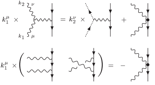
Figure 12: The tree-level version of the fundamental $s$-$t$ channel cancellation.

(iii) The effective gauge-independent Green’s function constructed by the PT coincide to all orders with the the background field method Green’s functions when the latter are computed in the (quantum) Feynman gauge [49, 50].

(iv) The equality of Eq (5.10) persists to all orders: after all gauge-cancellation have been carried out, the gauge-independent PT fermion self-energy coincides with the conventional one computed in the renormalizable Feynman gauge. The general statement of (iii) is of course valid in this case as well, simply because the fermion self-energy computed in the renormalizable Feynman gauge happens to be identical (to all orders) to the fermion self-energy computed in the background field method Feynman gauge. This last statement is of course not true in general; Green’s functions computed in the renormalizable Feynman gauge do not coincide with the corresponding Green’s functions computed in the background field method Feynman gauge. What is always true however is (iii).

(v) In QED (but not in QCD) the statement of (iv) is true also for the off-shell photon-fermion vertex $\Gamma_{\mu}$.

References

- [1] M. C. Diamantini, P. Sodano, E. Langmann and G. W. Semenoff, Nucl. Phys. B 406, 595 (1993) [arXiv:hep-lat/9301014].
- [2] N. Dorey and N. E. Mavromatos, Phys. Lett. B 250, 107 (1990); N. Dorey and N. E. Mavromatos, Nucl. Phys. B 386, 614 (1992); N. E. Mavromatos, Nucl. Phys. Proc. Suppl. 33C, 145 (1993).
- [3] A. Kovner and B. Rosenstein, Phys. Rev. B42, 4748 (1990).
- [4] D. H. Kim and P. A. Lee, Annals Phys. 272, 130 (1999) [arXiv:cond-mat/9810130] and references therein; L. Balents, M.P.A. Fisher and C. Nayak, Int. J. Mod. Phys. B10, 1033 (1998); Phys. Rev. B60, 1654 (1999).
- [5] M. Franz, Z. Tesanovic and O. Vafek, Phys. Rev. B 66, 054535 (2002) [arXiv:cond-mat/0203333]; see also [4],[6].
- [6] I. F. Herbut, Phys. Rev. B 66, 094504 (2002) [arXiv:cond-mat/0202491].
- [7] P.W. Anderson, Science 235, 1196 (1987); G. Baskaran and P.W. Anderson, Phys. Rev. B37, 580 (1988).
- [8] L.B. Ioffe and P.W. Wiegmann, Phys. Rev. Lett. 65 (1990), 653.
- [9] J. Frohlich and P. A. Marchetti, Phys. Rev. 46, 6535 (1992); J. Frohlich, T. Kerler and P. A. Marchetti, Nucl. Phys. B 374, 511 (1992).
- [10] T. Appelquist, A. G. Cohen and M. Schmaltz, Phys. Rev. D 60, 045003 (1999) [arXiv:hep-th/9901109].
- [11] J. M. Cornwall, Phys. Rev. D 26, 1453 (1982).
- [12] J. M. Cornwall and J. Papavassiliou, Phys. Rev. D 40, 3474 (1989).
- [13] K. Farakos and N. E. Mavromatos, Phys. Rev. B57, 3017 (1998). [arXiv:cond-mat/9611072]; N. E. Mavromatos and Sarben Sarkar, Int. J. Mod. Phys. B 17, 251 (2003) [arXiv:cond-mat/0210248], and references therein.
- [14] P.A. Lee, N. Nagaosa, T-K. Ng and X-G. Wen, Phys. Rev. B57, 6003 (1998).
- [15] R. Shankar, Phys. Rev. Lett. 63, 203 (1989); Nucl. Phys. B330, 433 (1990).
- [16] J. Alexandre, N. E. Mavromatos and Sarben Sarkar, Int. J. Mod. Phys. B 17, 2359 (2003) [arXiv:cond-mat/0303611]; New J. Phys. 5, 25 (2003) [arXiv:hep-th/0207232]; New J. Phys. 4, 24 (2002) [arXiv:hep-th/0202047].
- [17] B. Rosenstein, B. Warr and S. H. Park, Phys. Rev. Lett. 62, 1433 (1989); Phys. Rept. 205, 59 (1991).
- [18] R. Pisarski, Phys. Rev. D29, 2423 (1984); T. Appelquist, M. Bowick, D. Karabali, and L.C.R. Wijewardhana, Phys. Rev. D 33, 3704 (1986); T. Appelquist, D. Nash and L.C.R. Wijewardhana, Phys. Rev. Lett. 60, 2575 (1988).
- [19] C. Vafa and E. Witten, Nucl. Phys. B 234, 173 (1984); Comm. Math. Phys. 95, 257 (1984).
- [20] K. Farakos and N. E. Mavromatos, Int. J. Mod. Phys. B12, 809 (1998) [arXiv:cond-mat/9710288].
- [21] A. M. Polyakov, Nucl. Phys. B 120, 429 (1977).
- [22] M. J. Case, B. H. Seradjeh and I. F. Herbut, arXiv:cond-mat/0308260; I. F. Herbut and B. H. Seradjeh, Phys. Rev. Lett. 91, 171601 (2003) [arXiv:cond-mat/0305296]; F. S. Nogueira, J. Smiseth, E. Smorgrav and A. Sudbo, arXiv:hep-th/0310100.
- [23] I. Affleck, J. A. Harvey and E. Witten, Nucl. Phys. B 206, 413 (1982).
- [24] A. B. Zamolodchikov, JETP Lett. 43, 730 (1986) [Pisma Zh. Eksp. Teor. Fiz. 43, 565 (1986)].
- [25] K. i. Kondo and H. Nakatani, Prog. Theor. Phys. 87, 193 (1992); K. I. Kondo and T. Murakami, Phys. Lett. B 410, 257 (1997) [arXiv:hep-ph/9708260].
- [26] J. Papavassiliou and A. Pilaftsis, Phys. Rev. D 54, 5315 (1996) [arXiv:hep-ph/9605385].
- [27] J. Papavassiliou, E. de Rafael and N. J. Watson, Nucl. Phys. B 503, 79 (1997) [arXiv:hep-ph/9612237].
- [28] M. Binger and S. J. Brodsky, arXiv:hep-ph/0310322.
- [29] I. J. R. Aitchison, N. Dorey, M. Klein-Kreisler and N. E. Mavromatos, Phys. Lett. B 294, 91 (1992) [arXiv:hep-ph/9207246]; I.J.R. Aitchison and N.E. Mavromatos, Physical Review B 53, 9321 (1996); I.J.R. Aitchison, G. Amelino-Camelia, M. Klein-Kreisler, N.E. Mavromatos, and D. Mc Neill, Phys. Rev. B56, 2836 (1997); I. J. R. Aitchison, N. E. Mavromatos and D. McNeill, Phys. Lett. B 402, 154 (1997) [arXiv:hep-th/9701087].
- [30] V. P. Gusynin and M. Reenders, Phys. Rev. D 68, 025017 (2003) [arXiv:hep-ph/0304302].
- [31] J. M. Cornwall, R. Jackiw and E. Tomboulis, Phys. Rev. D 10, 2428 (1974).
- [32] J. M. Cornwall and D. A. Morris Phys. Rev D 52, 6074 (1995).
- [33] J. Papavassiliou and J. M. Cornwall, Phys. Rev. D 44, 1285 (1991).
- [34] N. E. Mavromatos and J. Papavassiliou, Phys. Rev. D 60, 125008 (1999).
- [35] Emden, Gaskugeln; R.H. Fowler, Quarterly Journal 45, 289 (1914); Quarterly Journal Oxford 2, 259 (1931).
- [36] E. Kamke, Differentialgleichungen, Lösungsmethoden und Lösungen (Akademische Verlagsgesellschaft, Geest & Portig K.G., Leipzig 1959).
- [37] S. J. Hands, J. B. Kogut and C. G. Strouthos, Nucl. Phys. B 645, 321 (2002) [arXiv:hep-lat/0208030] and references therein.
- [38] N. E. Mavromatos and Sarben Sarkar, Phys. Rev. B 62, 3438 (2000) [e-Print Archive: cond-mat/9912323].
- [39] A. Campbell-Smith, N. E. Mavromatos and J. Papavassiliou, Phys. Rev. D 60, 085002 (1999) [arXiv:hep-th/9905132].
- [40] W. J. Marciano and H. Pagels, Phys. Rept. 36, 137 (1978).
- [41] K. Johnson, M. Baker and R. Willey, Phys. Rev. 136 (1964) B1111; S. L. Adler and W. A. Bardeen, Phys. Rev. D 4 (1971) 3045 [Erratum-ibid. D 6 (1971) 734]; T. Maskawa and H. Nakajima, Prog. Theor. Phys. 52 (1974) 1326; 54 (1975) 860; V. A. Miransky, Phys. Lett. B 91 (1980) 421; P. I. Fomin, V. P. Gusynin, V. A. Miransky and Y. A. Sitenko, Riv. Nuovo Cim. 6N5 (1983) 1.
- [42] K. D. Lane, Phys. Rev. D 10 (1974) 2605; K. Higashijima, Phys. Rev. D 29 (1984) 1228; H. Pagels, Phys. Rev. D 19 (1979) 3080; D. Atkinson and P. W. Johnson, Phys. Rev. D 37 (1988) 2290; C. D. Roberts and B. H. McKellar, Phys. Rev. D 41 (1990) 672.
- [43] For example, T. Appelquist, D. Carrier, L. C. Wijewardhana and W. Zheng, Phys. Rev. Lett. 60 (1988) 1114; T. Appelquist, K. D. Lane and U. Mahanta, Phys. Rev. Lett. 61 (1988) 1553.
- [44] C. N. Leung, S. T. Love and W. A. Bardeen, Nucl. Phys. B 323 (1989) 493.
- [45] D. K. Hong, V. A. Miransky, I. A. Shovkovy and L. C. Wijewardhana, Phys. Rev. D 61, 056001 (2000) [Erratum-ibid. D 62, 059903 (2000)] [arXiv:hep-ph/9906478].
- [46] W. A. Bardeen, C. T. Hill and M. Lindner, Phys. Rev. D 41, 1647 (1990).
- [47] V. Sauli, JHEP 0302, 001 (2003) [arXiv:hep-ph/0209046].
- [48] D. Binosi and J. Papavassiliou, Phys. Rev. D 65, 085003 (2002)
- [49] D. Binosi and J. Papavassiliou, Phys. Rev. D 66, 111901 (2002)
- [50] D. Binosi and J. Papavassiliou, arXiv:hep-ph/0301096.