Metastable liquid lamellar structures in binary and ternary mixtures of Lennard-Jones fluids

Abstract

We have carried out extensive equilibrium molecular dynamics (MD) simulations to investigate the Liquid-Vapor coexistence in partially miscible binary and ternary mixtures of Lennard-Jones (LJ) fluids. We have studied in detail the time evolution of the density profiles and the interfacial properties in a temperature region of the phase diagram where the condensed phase is demixed. The composition of the mixtures are fixed, 50% for the binary mixture and 33.33% for the ternary mixture. The results of the simulations clearly indicate that in the range of temperatures $78<T<102~{}^{\rm o}$K, –in the scale of argon– the system evolves towards a metastable alternated liquid-liquid lamellar state in coexistence with its vapor phase. These states can be achieved if the initial configuration is fully disordered, that is, when the particles of the fluids are randomly placed on the sites of an FCC crystal or the system is completely mixed. As temperature decreases these states become very well defined and more stables in time. We find that below $90~{}^{\rm o}$K, the alternated liquid-liquid lamellar state remains alive for 80 ns, in the scale of argon, the longest simulation we have carried out. Nonetheless, we believe that in this temperature region these states will be alive for even much longer times.

I introduction

In the past decade there has been a growing interest in studying the structure and interfacial properties of the liquid-liquid (LL) and liquid-vapor (LV) phase coexistence of binary and ternary mixtures of simple fluids. The reason for this is that they are of fundamental importance to understand the behavior of more complex fluids. A few examples where a better understanding of these phenomena may have impact are, in the design, operation and optimization of the extraction processes, in tertiary oil recovery, in the adsorption or coating processes, in biological processes, etc. Different analytical approaches dagamma1 ; tarazona1 ; jlee1 ; almeida , and density functional theory implementations wendall ; fortsman97 ; nader2002 , as well as numerical simulationschapela ; salomons ; holcomb ; li95 ; mecke99 ; alejandre99 ; diaz99 have been used to investigate these issues in simple fluids and in more complex systems strey95 ; guerra98 ; endo2000 ; isamu2001 . Binary mixtures of LJ fluids have been investigated with the aim at understanding the phase coexistence as well as the interfacial and structural properties of the LV and LL interfaces. The dependence of the surface tension on the composition of the bulk phases and surface segregation at the LV interface have also been analyzed jlee1 ; salomons ; nijmeijer88 . For two immiscible LJ fluids the structure of the LL interface, the capillary waves and pressure effects on the interfacial tension have also been studied toxvaerd95 ; stecki95 ; padilla96 . In addition, the structure of LV and LL interfaces in binary mixtures of LJ fluids have been investigated using density functional theory fortsman97 as well as molecular dynamics simulations mecke99 . In the present paper we have investigated the time evolution of the density profiles and interfacial properties of binary and ternary mixtures of partially miscible LJ fluids in a temperature region of the phase diagram where the condensed phase is demixed. The phase diagram that better describes our model binary mixture is one that has the usual low temperature triple point and a higher temperature triple point where the vapor phase coexists with a mixed and a demixed liquid phases wilding97 . These types of mixtures have received attention until recently and need to be studied more extensively. Our findings indicate that by properly tuning the temperature, $78<T<102~{}^{\rm o}$K, –in the scale of argon– and the interactions between the species, long lived metastable alternated lamellar states in the liquid-liquid phase coexist with the vapor phase. These states are found in binary and ternary mixtures at compositions of 50%, and 33.33%, respectively. As temperature decreases these states become sharper and more stables in time. We find that below $90~{}^{\rm o}$K, the alternated liquid lamellar state remains alive for at least 80 ns in the scale of argon. This is the longest simulation that we have carried out. However, we believe that below this temperature these states will remain there for even very long times, suggesting that the alternated liquid-liquid phases are a manifestation of the existence of a number of local equilibria. The layout of the remainder of this paper is as follows. In section II we describe the model potentials that define the type of mixtures that we have investigated. Then we continue in section III with a description of the parameters of the MD simulations. The results and discussion of them are presented in section IV. Finally, we end the paper with the conclusions that are in section V.

II The models.

Let us start this section by defining the model system for the binary fluid mixture. This is made up of spherical particles A and B that interact between themselves through a LJ potential defined by

$$u_{ij}=4\epsilon_{ij}\left[\left(\frac{\sigma_{ij}}{r_{ij}}\right)^{12}-\left(\frac{\sigma_{ij}}{r_{ij}}\right)^{6}\right],$$ (1)

where i,j=A,B. We will use $\sigma_{AA}$ and $\epsilon_{AA}$ as the reference parameters, that is, $\epsilon_{ij}=\epsilon_{AA}\alpha_{ij}$ and $\sigma_{ij}=\sigma_{AA}=1.0$. This choice of parameters represents a system in which all the particles are of equal size and the interactions are tuned by properly choosing the elements of the symmetrical matrix $\alpha_{ij}$. Since we want to study a partially miscible binary mixture the attractive part of the interaction potential between particles of fluids A and B is chosen to be weaker than the attraction between particles of the same specie. Therefore all the matrix elements $\alpha_{ij}$ are equal to unity except those corresponding to the crossed AB interactions that are $\alpha_{AB}$=0.75. This choice of potential favors the demixing of fluids A and B. On the other hand, the ternary mixture we have considered is formed by fluids A, B and C which particles are of the same size for the three fluid components. The potential interactions between fluids of different kind are chosen such that they favor the mixing of the pairs of fluids B,C and A,C (alike interactions). However, the A-B fluids interactions disfavor their mixing (unlike interactions). Bearing this in mind we can define the interaction potential in a similar way as we did for the binary mixture. It is defined by Eq. 1 where i,j=A,B,C, and the matrix elements $\alpha_{ij}$ are equal to unity for particles of the same type as well as the crossed interactions BC and AC. Nonetheless, the AB crossed interactions have matrix elements $\alpha_{AB}=0.75$. With this choice of potentials, fluid C may be considered as a surfactant. The reason for this is that particles of fluid C mediate the unlike A-B fluids interactions, that is, particles of fluid C interact favorably with particles of fluids A and B, while particles of fluids A and B interact unfavorably diaz99 . In the following section we present information concerning the parameters and details of the numerical simulations.

III Parameters and description of the simulations.

We have carried out extensive equilibrium molecular dynamics simulations in the (N,V,T) ensemble. In each time step iteration we monitor the temperature of the system via the equipartition theorem and rescale the linear momentum of the particles to keep the temperature constant. In all the simulations performed in this work the interparticle potentials have been shifted in such a way that they are equal to zero right at the cutoff $r_{c}=3\sigma_{AA}$. It has been shown that this cutoff is the appropriate to account for the long tail of the potential alejandre99 . We have simulated systems with as many as 4096 particles for the binary mixture and 8192 particles for the ternary mixture. They are located inside a parallelepiped of volume $12\sigma_{AA}\times 12\sigma_{AA}\times L_{z}$, with $L_{z}>12\sigma_{AA}$. We have applied periodic boundary conditions in all three directions. To minimize finite size effects in the interfacial properties we have followed reference li95 . There it is shown that in order to have interfacial properties independent of the size of the area it should be at least $12\sigma_{AA}\times 12\sigma_{AA}$. We have found that for the type of mixtures –interactions– studied in this work the choice of the initial configuration is crucial so we leave this discussion for the next section. At this point all we can say is that the initial velocities of the particles are chosen from an equilibrium Boltzmann distribution. The thermodynamic variables used to describe the system’s behavior are, the reduced temperature $T^{*}=\frac{k_{{}_{B}}T}{\epsilon_{AA}}$ with $k_{{}_{B}}=$ Boltzmann’s constant and the reduced density $\rho^{*}={{\rho}{\sigma_{AA}^{3}}}$. To investigate the interfacial properties we need to define the reduced interfacial tension, $\gamma^{*}=(\sigma^{2}_{AA}/\epsilon_{AA})\gamma$. The total density of the system is given by $\rho=N/V$, where $N$ is the total number of particles and $V$ is the volume of the system. The equations of motion that describe the dynamics of the particles of the fluids are solved using a leap-frog scheme with an integration step-size $\Delta t^{*}\leq 5\times 10^{-3}$. To be able to compare the time scale and temperatures of our simulations in the remaining of this paper we will use as a reference scale that corresponding to argon. In this scale the time step is equal to $1.1\times 10^{-5}$ nanoseconds (ns). The shortest equilibration times that we considered in the simulations were of the order of $5\times 10^{5}$ time steps (5.5 to 11 ns) and the total length of the simulations after equilibration is in the range of 4-7 million time steps (5.5 to 11 ns). To minimize correlations between measurements we calculated thermodynamic and structural quantities every 50 time steps. Since we want to study the liquid-vapor phase coexistence the total density of the system has been chosen to be right inside the LV coexistence curve. In this way we are able to study directly the structural properties of the interfaces and explicitly obtain the distribution of the species in the directions parallel and perpendicular to the interfaces.

IV Results and discussion.

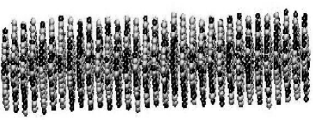
Figure 1: Snapshot of the binary mixture “disordered initial configuration”. At $t=0$ the particles of fluids A (black) and B (gray) are randomly located on the sites of an FCC crystal.

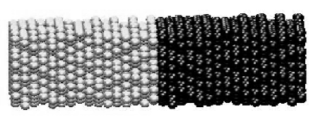
Figure 2: Snapshot of the binary mixture “ordered initial configuration”. At $t=0$ the particles of fluids A (black) and B (gray) are separated and located on the sites of two adjacent FCC crystals.

We would like to recall that our main objective is to focus on the time evolution of the demixed liquid-liquid-vapor (LLV) phase coexistence of the binary mixture whose phase diagram is described in reference wilding98 . These types of mixtures have received much less attention than those based on the Lorentz-Berthelot rule that usually yield a mixed liquid phase. We have found that in the partially miscible mixtures studied here, care should be exercised when choosing the initial configuration of the simulations since there are long lived metastable states. It is known that an equilibrium state can be reached from any two different initial configurations. Nonetheless, for practical purposes, one always chooses an initial configuration that is close to the expected equilibrium state. So, in the case of a partially miscible mixture it is natural to start from a configuration in which the species are separated if one expects to obtain a demixed liquid state. On the contrary, if in the final equilibrium state the liquids are mixed then one should initiate the simulation from a mixed configuration. In this paper we show evidence that long lived metastable alternated liquid-liquid lamellar states in coexistence with the vapor phase can be achieved if the simulations start from a “disordered initial configuration” defined as one in which fluids A and B are fully mixed in the liquid-liquid phase or their particles are randomly located on the sites of an FCC crystal, as it is shown in Fig. 1. However, if we start the simulations from an “ordered initial configuration” defined as one in which the particles of fluids A and B are placed on the sites of two adjacent FCC crystals or they are distributed on two contiguous slabs containing fluids A and B respectively, as shown in Fig. 2, the system ends up in an equilibrium configuration where the distribution of fluids essentially remains the same as in the initial configuration.

To allow the formation of the vapor phase in the MD simulations we have left a free volume on both sides of the initial distribution of particles. However, this empty space is not shown in the snapshots. In the next two subsections we show and discuss the results of the time evolution of a binary and a ternary mixtures.

IV.1 Binary mixture.

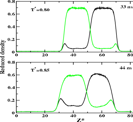
Figure 3: Density profiles of the binary mixture in the demixed liquid state in coexistence with the vapor phase. Notice that the density profiles of the fluid phase that is less rich show a peak structure close to the LV interface. See text for an explanation of this result.

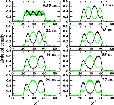
Figure 4: Density profiles for the mixed condensed state of the system in coexistence with its vapor phase at $T^{*}=0.85$.

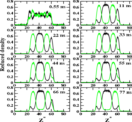
Figure 5: Density profiles for the mixed condensed state of the system in coexistence with its vapor phase at $T^{*}=0.80$.

Let us start by considering a typical LLV interface structure when the simulation begins from an “ordered configuration” as that shown in Fig. 2. The mixture has a total of 4096 particles with a concentration of fluids A and B of 50%. We have considered an average particle density of $\rho^{*}_{\rm tot.}=\rho^{*}_{A}+\rho^{*}_{B}=0.35$. In figure 3 we show the density profiles of the LLV coexistence at the reduced temperatures $T^{*}=0.85$ and $0.80$. In our reference scale these temperatures correspond to $T=101.83~{}^{\rm o}$K, and $T=95.84~{}^{\rm o}$K, respectively, and are in the demixing region of the phase diagram wilding98 . Therefore we obtain two partially separated liquid phases, one rich in fluid A and the other rich in fluid B and both of them in coexistence with the vapor phase. Notice that this is the minimum number of interfaces that one can obtain using periodic boundary conditions. Observe that in the phase of fluid A or B one can also find fewer amounts of fluid B or A, whose average density is small and constant in the bulk phase and develops a peak structure at the LV interfaces as can be seen in density profiles. This distribution of particles occurs as a consequence of the difference in the local densities and the unlike potential interactions between the fluids. It is important to point out that this kind of structure can only be obtained by means of the construction of the interfaces as we have done in the present MD simulations. Another important fact to bear in mind is the amount of simulational time required to obtain the equilibrium density profiles such that the two liquid phases are completely symmetric. So we needed to simulate these systems for as long as 33 ns and 44 ns at each one of these two temperatures, respectively. On the other hand, figures 4 and 5 show the time evolution of the density profiles of the mixture at the same temperatures, $T^{*}=0.85$ and $0.80$. When the simulations started from a “disordered initial configuration” as the one shown in Fig. 1 we observe that at both temperatures, and at the early stages of the time evolution, $11$ ns, the system clearly shows the signature of an alternated A-rich and B-rich liquid lamellar structure in coexistence with the vapor phase. One would expect that the number of lamellae should be proportional to the number of particles in the system. To test the time stability of these alternated structures we performed quite long MD simulations, as long as $77$ ns for each temperature. The time length of these simulations is about 1.75 to 2.3 times longer than the time we followed the evolution of the systems initiated from an “ordered initial configuration”, that in turn yielded the structure shown in Fig. 3. We find that at high temperatures the lifetime of the lamellar structure is relatively short because the kinetic energy overcomes easily the LL interfacial energy barrier. In Fig. 4 it is seen that for $T^{*}=0.85$ one of the lamellae has dissapeared at 33 ns. Nonetheless, at a lower temperature $T^{*}=0.80$ the time required for this disappearance to occur is between 66-77 ns, about two times longer than at $T^{*}=0.85$. This is due to the diffusion of particles from the narrowest lamella that becomes unstable, in this case, the one on the right hand side, towards the lamella at the middle, that in turn becomes thicker. The fact that the right hand side lamella is the narrowest is due to a local density fluctuation in the system. However, this local density fluctuation may also occur in any one of the lamellae. To understand why this diffusion of particles occurs in this direction and not in the direction of the vapor phase we estimated the LV and LL interfacial energies at both temperatures. In doing so we integrated the difference between the normal and tangential pressure profiles diaz99 . One more test of the reliability of the simulations is to check that this difference is zero in the bulk phases and that the normal pressure is constant through the length of the simulational parallelepiped. Our results indicate that the LV interfacial tensions $\gamma^{*}_{LV}(T^{*}=0.85)=0.290\pm 0.005$ and $\gamma^{*}_{LV}(T^{*}=0.80)=0.420\pm 0.006$) are significantly greater than those corresponding to the LL interfacial tensions ($\gamma^{*}_{LL}(T^{*}=0.85)=0.07\pm 0.01$ and $\gamma^{*}_{LL}(T^{*}=0.80)=0.150\pm 0.001$). Consequently, the fluid particles forming the lamella at the right end of the LL structure have to diffuse towards the liquid lamellar phase since more energy is required to move towards the vapor phase.

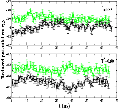
Figure 6: Time evolution of the potential energy of the mixture at reduced temperatures $T^{*}=0.85\>{\rm and}\>0.80$. The data in gray color correspond to a demixed fluid phase configuration while the data in black correspond to an ordered initial configuration.

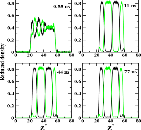
Figure 7: Density profiles for the mixed condensed state of the system in coexistence with its vapor phase at $T^{*}=0.65$. Note that in the bulk phase, but close to the LV interface, the density profile of fluid C shows peaks as a consequence of the unlike interactions between the A and B particles.

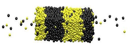
Figure 8: Snapshot of the particles arrangement in the long lived alternated lamellar state in coexistence with its vapor phase at $T^{*}=0.65$ at 77 ns of the simulation.

To show that the system at $T^{*}=0.85$ has a shorter lifetime and eventually will end up forming two liquid slabs in coexistence with the vapor phase we followed the time evolution of the potential energies when the simulations are started from an ordered and a disordered configurations. The results are plotted in Fig. 6 where one sees that for $T^{*}=0.85$ the behavior of the potential energy is such that after about $t_{a}=27.5$ ns both curves are very close to each other within the size of the error bars. This indicates that for $t>t_{a}$ the potential energies of both systems are the same within the accuracy of the simulations, suggesting that in both cases the system is approaching the same thermodynamic state. However, this appears not to be the case for $T^{*}=0.80$ in which case the time evolution of the potential energy indicates that the curves are clearly separated when the initial configurations are different. Thus one can say that the system may converge to two possible states. One in which the free energy is minimum, –just one LL interface– and the other with many LL interfaces –alternated lamellar state– whose free energy appears not to be the minimum due to the existence of several interfaces. As we decrease further the temperature we find that the liquid lamellar state becomes very well defined –sharper– and more stable. In Figure 7 we show the time evolution of the density profiles at the reduced temperature $T^{*}=0.65$ where once more, the simulations started from a disordered configuration. It is important to note that if the simulation starts from an ordered configuration then the system ends up forming two separated liquid slabs in coexistence with the vapor phase. At this temperature the alternated lamellar structure is very well defined at early times of the simulations ($t=11$ ns). Notice that in this case the LL interfaces are sharper and the width of the lamellae is narrower and very well defined as compared to those obtained at higher temperatures. Note that the simulations are quite long, $77$ ns and the structure is stable during all this time. This is not totally unexpected since as temperature decreases the diffusion of the particles of fluid A in the phase of fluid B decreases as a consequence of the values of the interfacial tension of the LL interface, $(\gamma^{*}_{LL}=0.46\pm 0.02)$. This value is about 6.6 times greater than the value of $\gamma^{*}$ at $T^{*}=0.85$. In Fig. 8 we show a snapshot of the system at $T^{*}=0.65$ after 77 ns of the simulation. There one can see explicitly the lamellar structure whose density profiles are shown in the fourth panel of Fig. 7. In the next subsection we address the issue of how a surfactant fluid –third specie– affects the stability of the lamellar state of the binary mixture at $T^{*}=0.65$.

IV.2 Ternary mixture

Let us now consider a ternary mixture of fluids A, B and C such that fluids A and B are partially miscible, unlike interactions, while the other possible mixtures are miscible, that is, the A-C and B-C interactions are alike. Therefore, all the matrix elements $\alpha_{i,j}$ of the interparticle potential, Eq. 1, are equal to unity except those corresponding to the A-B interactions for which $\alpha_{A,B}=0.75$, as defined in section II. Here the concentrations of fluids A,B and C are approximately one third of the total concentration,that is, $C_{A}=C_{B}=C_{C}\simeq 33.33\%$. In order to obtain a well defined lamellar state –at least four lamellae– with these concentrations we needed a total of 8192 particles of which 2730 particles correspond to fluid C and 2731 for the other two fluids. As a consequence of the increase in the number of particles the calculations become very demanding and the the CPU time increases substantially. As indicated at the beginning of this section to study the time evolution of the mixture we considered an “ordered” and a “disordered” initial configurations, as described in what follows. The ordered initial configuration was obtained from the two LL slabs in coexistence with the vapor phase of the binary mixture at $T^{*}=0.65$ and the particles of the third specie were taken from the two liquid slabs. The disordered initial configuration is defined as one in which the particles of the three fluids are randomly placed on the sites of an FCC crystal. For each initial configuration the mixture was simulated for as long as 55 ns. Fig. 9 shows the time evolution of the density profiles when the simulation initiated from a random configuration. Each panel represents the average of the density profiles over 11 ns. One sees that a pretty well defined alternated liquid A-liquid B lamellar state with the number of lamellae constant is reached. In addition, one observes that the distribution of fluid C is uniform at the liquid phases. However, its concentration increases at the LL interfaces. This is consistent with a recent study as reported in reference diaz99 . Because of this the interfacial tension of the LL interface decreases significantly as compared to the corresponding values of the binary mixture, as will be shown below. On the other hand, Fig. 10 shows the time evolution of the mixture when the simulation started from an ordered configuration. One sees that the basic structure of the initial configuration remains stable in time with the surfactant uniformly distributed in the liquid phases and an increase in concentration at the LL interface. This distribution of fluid C is similar to that found in the alternated lamellar state. The oscillations that are seen in the density profiles are mainly due to local fluctuations of the concentration since a rearrangement of the fluid particles is taking place. One would expect that after a very long time the system will eventually end up forming two separated liquid slabs of the same width in coexistence with the vapor phase. At this point we are not able to indicate clearly which one of these states corresponds to the equilibrium state because it is very difficult to evaluate explicitly the free energy of the system. To try to circumvent this difficulty we proceed as in the binary mixture case, that is, we follow the time evolution of the potential energy for both structures at $T^{*}=0.65$ and the results are plotted in Fig. 11. In the upper panel we observe that the lines representing the potential energies are pretty close to each other within the error bars. To see which system has more potential energy we removed the error bars from these curves. The curves are plotted in the lower panel of the same figure where we observe that for most of the time of the simulations the potential energies are essentially the same within the accuracy of the calculations. This may be an indication that both states are approaching the same thermodynamic state. To try to clarify this issue we proceed further and evaluate the interfacial energy per unit area of both states. To evaluate the reduced interfacial tension we used the Kirwood-Buff formula kirwood-buff that has proved to give reasonable estimates diaz99 . The results of this calculation for the liquid-vapor plus liquid-liquid interfaces are plotted as a function of time for both configurations in Fig. 12. In the upper panel one can observe that the interfacial tension shows strong fluctuations in both cases. To understand the time evolution of $\gamma^{*}$ we carried out a smoothing procedure of the data and the results are shown in the lower panel of the figure. In doing so we averaged $\gamma^{*}$ every four points. We observe that for both configurations the trend in $\gamma^{*}$ is about the same, however, the interfacial tension of the lamellar state is systematically above the the interfacial tension of the two liquid slabs system. The time average difference of this quantity is about $0.13$. It is important to point out that the difference between the total interfacial tensions of these two states comes mainly from the LL interfaces since the LV interfacial tensions are similar and thus cancell out. The decrease in $\gamma^{*}$ relative to the binary system is due to the surfactant character of the fluid C which concentration is slightly higher at the LL interfaces. These results for the potential and interfacial energies indicates that in spite of the surfactant character of fluid C, the alternated LL lamellar state remains stable for quite a long time. This happens because there should be an energy barrier that is large enough to be overcome by the system when the initial configuration of fluids A,B and C is fully random. Therefore, our results strongly suggest that the alternated LL lamellar state is a long lived metastable state even in the case when fluid C plays the role of a surfactant. Of course as one would expect, if the concentration of fluid C increased one should reach a concentration at which the lamellar state would become into two liquid A liquid B slabs. Increasing further the concentration of C would finally lead to a mixed state.

V Conclusions.

We have shown from extensive MD simulations that by properly choosing the interaction parameters of the interparticle potentials and the initial conditions, long lived metastable alternated LL lamellar states can be achieved in partially miscible binary and ternary mixtures of LJ fluids. These lamellar states are found to be stable and sharper at relatively low temperatures, in the temperature range of the fluid phase ($78-102~{}^{\rm o}$K). At temperatures well above $102~{}^{\rm o}$K we obtain a mixed liquid phase in coexistence with the vapor and the mixture reaches relatively easy the equilibrium state. However, at temperatures below this value the liquid phase of the system is demixed and relaxes slowly to the equilibrium state. We have also found that for disordered initial conditions we obtain long lived LL alternated lamellar states. One important question to be answered in a future research is how is related the number of lamellae with the number of local equilibria. For the ternary mixture that is essentially formed by the partially miscible binary mixture and a surfactant fluid, we have found that even in this case pretty stable long lived alternated liquid-liquid lamellar structures can be achieved by considering a disordered the initial state as well. The alternated LL lamellar structures found here are more or less similar to those obtained in a recent density functional study of the LV coexistence of amphiphile dumbells in coexistence with a LJ fluid nap00 . Nonetheless, in this latter case the alternated lamellar state constitutes an equilibrium state. Bearing in mind this model one may consider the ternary mixture studied in the present paper as one in which particles B-C (or A-C) form effective amphiphile-like molecules interacting with fluid A (or B). It is important to stress the fact that here we have obtained these LL lamellar structures in coexistence with the vapor phase by considering spherical single particle LJ fluids. Nevertheless, these appear to be long lived metastable states that are stable and sharper in time at relatively low temperatures.

VI Acknowledgements

EDH would like to acknowledge enlightening discussions with F. Forstmann. This work has been supported by CONACYT research grants Nos. L0080-E (EDH), and 25298-E, G32723-E (GRS).

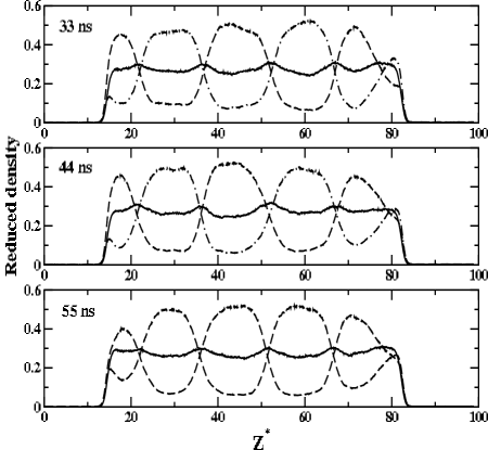
Figure 9: Time evolution of the density profiles of the lamellar state at $T^{*}=0.65$. Averages are calculated using three subsequent blocks of one million time steps each. The initial configuration is disordered.

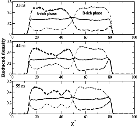
Figure 10: Time evolution of the density profiles of the lamellar state at $T^{*}=0.65$. Averages are calculated using three subsequent blocks of one million time steps each. Here the system started from an ordered configuration. Notice that in the third block the density profiles of fluid A show oscillations.

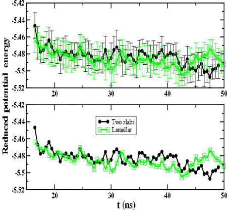
Figure 11: Time evolution of the potential energy of the mixture at $T^{*}=0.65$.

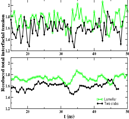
Figure 12: Upper figure shows the time evolution of the interfacial energy and its fluctuations for both, the alternated lamellar and the two liquid slab state in coexistence with the vapor phase. The large size of the fluctuations is mainly attributed to the relatively high concentration of fluid C at the LL interfaces. In the lower figure we show the same quantity after a smoothing process has taken place. As a result one sees that on the average, the lamellar state has a consistently but slightly higher interfacial tension.

References

- (1) M.M. Telo da Gamma and R. Evans, Mol. Phys. 41, 1091 (1980), ibid, Faraday Symp. Chem. Soc. 16, 45 (1981).
- (2) P. Tarazona, M.M. Telo da Gamma and R. Evans, Mol. Phys. 49, 283 (1983), ibid, 49, 301 (1983).
- (3) J. Lee, M.M. Telo da Gamma and K. E. Gubbins, Mol. Phys. 53, 1113 (1984), ibid J. Phys. Chem. 89, 1514 (1985).
- (4) B. S. Almeida and M.M. Telo da Gamma J. Phys. Chem. 93,4132 (1989).
- (5) M. Wendland, Fluid Phase Equilibria 141, 25 (1997), ibid, 147, 105 (1998).
- (6) Stanislav Iatsevitch and Frank Forstmann, J. Chem. Phys. 107, 6925, (1997).
- (7) N. Lotfohalli, Mohammad, Modarres, Hamid, J. Chem. Phys. 166, 2487 (2002).
- (8) G. A. Chapela, G. Saville, S. M. Thompson, and J. S. Rowlinson, J. Chem. Soc., Faraday Trans. 2 73, 1133 (1977).
- (9) E. Salomons and M. Mareschal, J. Phys.: Condens. Matter 3, 3645 (1991), ibid, 3, 9215 (1991).
- (10) C. D. Holcomb, P. Clancy, S. M. Thompson, and J. A. Zolweg, Fluid Phase Equilibria 75, 185 (1992); ibid 88, 303 (1993); C. D. Holcomb, P. Clancy, and J. A. Zolweg, Mol. Phys. 78, 437 (1993).
- (11) Li-Jen Chen, J. Chem. Phys. 103, 10214 (1995).
- (12) M. Mecke and J. Winkelmann, J. Chem. Phys. 110, 1188 (1999).
- (13) Andrij Trokhymchuck and José Alejandre, J. Chem. Phys. 111, 8510, (1999).
- (14) Enrique Díaz-Herrera, José Alejandre, Guillermo Ramírez-Santiago and F. Forstmann, J. Chem. Phys. 110, 8084, (1999).
- (15) R. Strey, Y. Viisanen, and P. E. Wagner, J. of Chem. Phys. 103, 4333 (1995).
- (16) C. Guerra, A. M. Somoza and M.M. Telo da Gamma, J. Phys. Chem. 109, 1152 (1998).
- (17) H. Endo, M. Mihailescu, M. Monkenbusch, J. Allgaier, G. Gompper, D. Richter, B. Jakobs, T. Sottmann, R. Strey and I. Grillo, J. Chem. Phys. 115, 580 (2001).
- (18) I. Kusaka, D. W. Oxtoby, J. Chem. Phys. 115, 4883 (2001).
- (19) M.J.P. Nijmeijer, A. F. Bakker, C. Bruin, and J. H. Sikkenk, J. Chem. Phys. 89,3789 (1988).
- (20) S. Toxvaerd and J. Stecki, J. Chem. Phys. 102, 7163 (1995).
- (21) J. Stecki and S. Toxvaerd, J. Chem. Phys. 103, 4352 (1995); ibid. J. Chem. Phys. 103, 9763 (1995).
- (22) P. Padilla and J. Stecki, J. Chem. Phys. 104, 7249 (1996).
- (23) N. B. Wilding, Phys. Rev. E 55, 6624 (1997).
- (24) N. B. Wilding, F. Schmid, P. Nielaba, Phys. Rev. E 58, 2201 (1998).
- (25) Jian-Gang Weng, Seungho Park, Jennifer R. Lukes, and Chang-Lin Tien, J. Chem. Phys. 113, 5917, (2000).
- (26) J. G. Kirwood and F. P. Buff, J. Chem. Phys. 17, 338 (1949).
- (27) Ismo Napari and Ari Laaksonen, Phys. Rev. Lett. 84, 2184 (2000).