Plaquette operators used in the rigorous study of ground-states of the Periodic Anderson Model in $D=2$ dimensions.

Abstract

The derivation procedure of exact ground-states for the periodic Anderson model (PAM) in restricted regions of the parameter space and $D=2$ dimensions using plaquette operators is presented in detail. Using this procedure, we are reporting for the first time exact ground-states for PAM in 2D and finite value of the interaction, whose presence do not require the next to nearest neighbor extension terms in the Hamiltonian. In order to do this, a completely new type of plaquette operator is introduced for PAM, based on which a new localized phase is deduced whose physical properties are analyzed in detail. The obtained results provide exact theoretical data which can be used for the understanding of system properties leading to metal-insulator transitions, strongly debated in recent publications in the frame of PAM. In the described case, the lost of the localization character is connected to the break-down of the long-range density-density correlations rather than Kondo physics.

I Introduction

The periodic Anderson model (PAM) is one of the basic models describing strongly correlated systems whose characteristics fit to be interpreted in a two-band picture [1]. The model is largely applied in the study of heavy-fermion systems [2], intermediate-valence compounds [3], or even high critical temperature superconductors [4]. In contrast however with other models used in the understanding of phenomena created by strong correlation effects, where at least in one dimension exact solutions exist (for example the Hubbard model [5]), the physics described by PAM is almost exclusively interpreted based on approximations. This is due to the fact that only few results are exactly known about the behavior of PAM.

Indeed, what we know about the physical behavior of PAM in rigorous terms can be summarized as follows: The first results, related to the ground-state of decorated hyper-cubic lattices in the limit of infinite interaction strength has been provided by Brandt and Giesekus [6] followed by a non-magnetic ground-state restricted to 1D and on-site repulsion $U=\infty$ case obtained by Strack [7]. This solution has been extended to $D=2,3$ as well, at $U=\infty$ [8, 9]. Again for infinite on-site Hubbard repulsion has been demonstrated that at quarter filling the ground-state is unique with a defined total spin [10]. It has been also underlined that the model becomes solvable in the case of constant and infinite range hopping [11]. We further know, that for only on-site hybridization and without direct hopping in the correlated band: the symmetric half-filled case is spin-singlet [12] and in 1D also pseudo-spin singlet [13], at half filling anti-ferromagnetic correlations are present [14], and in 1D,2D long-range order of ferro, anti-ferro and pairing type is absent [15]. Recently have been published the first exact ground-states at finite $U$ in 1D [16, 17] and 2D [18], respectively. Concerning 2D, the reported ground-states [18] require next to nearest-neighbor (NNN) one-particle terms as well in the Hamiltonian ($\hat{H}$), and from the obtained solutions, especially the physical properties of the itinerant one has been described in detail.

The deduction of exact ground-states in $D=2$ dimensions is of large interest in general, and for strongly correlated systems in special. In the case of PAM, at finite and nonzero value of the interaction, the only one procedure doable working at the moment in this respect, is based on plaquette operators introduced in Ref.[18], and a decomposition of the on-site Hubbard interaction as described in Ref. [16]. During this procedure, $\hat{H}$ is such transformed to contain in a positive semidefinite form products of plaquette operators. Since in 2D the product of plaquette operators generates NNN one-particle terms as well, the general impression created by the method suggests that the applicability of the procedure is intimately connected to NNN contributions in 2D, and the deduced exact ground-states are fingerprints of this fact.

In this paper, presenting for the first time exact ground-states for PAM in 2D at finite value of the interaction, in restricted regions of the parameter space and without NNN type of extension terms in $\hat{H}$, we demostrate that the plaquette operator procedure and the ground-states deduced with it are not necessarily connected to the presence of NNN extensions in $\hat{H}$. In order to clarify these aspects (i) the plaquette operator technique is analysed in detail in general terms and 2D, (ii) a completely new type of plaquette operator is introduced which allows the deduction of the presented results, (iii) the obtained new localized exact ground-state is analyzed and described in detail, and (iv) implications of the results relating the metal-insulator transition in frame of PAM are presented.

The deduced new ground-state is a completely localized state. In order to characterize this phase, after obtaining the exact ground-state, all relevant ground-state expectation values and correlation functions have been exactly calculated and analyzed. The obtained state is paramagnetic, and based on a coherent control which it has on the occupation number of all lattice sites, it introduces long-range density-density correlations into the system, producing a localized state.

Concerning implications to physical systems, we mention the intense activity in the field related to the understanding of the metal-insulator transition (MIT) in frame of PAM. The subject has an almost 30 years of history [19], and gained renewed interest in the last period based on the observed MIT similarities between the Hubbard model and PAM, used for example in the understanding of the iso-structural electronically driven MIT transitions (like the $\gamma\to\alpha$ transition in $Ce$ compounds) [20, 21, 22, 23, 24, 25]. Since the exactly deduced ground-state energy values presented in this paper are not containing exponential factors characteristique to Kondo type of behavior, the results reported here underline that at least in some regions of the parameter space, a localization-delocalization transition in frame of PAM is not necessarily connected to Kondo physics.

The remaining part of the paper is structurated as follows: Section II. presents the Hamiltonian we use, Section III. describes the plaquette operator technique, Section IV. presents the transformation of the starting Hamiltonian into a new expression containing plaquette operators, Section V. describes the detected new exact ground-states, Section VI. concludes the paper, and Appendices A.- D. containing the mathematical details of the starting points of the paper close the presentation.

II The expression of the Hamiltonian.

We start with a generic PAM Hamiltonian written for 2D square lattice as

$$\hat{H}=\hat{T}_{d}+\hat{T}_{f}+\hat{E}_{f}+\hat{V}+\hat{U}\>,$$ (1)

where, the contributing terms in order, are representing the kinetic energy of $d$ electrons ($\hat{T}_{d}$), the kinetic energy of $f$ electrons ($\hat{T}_{f}$), the on-site $f$ electron energy ($\hat{E}_{f}$), the hybridization ($\hat{V}$), and the on-site Hubbard interaction written for $f$ electrons $\hat{U}=U\hat{U}_{f}$, the last contribution representing the interaction term, and $U>0$ being considered during this paper. The presence of $\hat{T}_{f}$ in $\hat{H}$ is motivated by the overwhelming evidence, that the heavy-fermion materials contain in their real band structure around the Fermi level ($E_{F}$) very narrow, hybridized bands, which exist already at temperatures far above the thermodynamically determined Kondo temperature, being relatively $T$ independent and holding an accentuate $f$ character [26].

The interaction term during this paper is exactly transformed in the form

$$\hat{U}_{f}=\sum_{i}\hat{n}^{f}_{i,\uparrow}\hat{n}^{f}_{i,\downarrow}=\hat{P}^{\prime}+\sum_{i}(\sum_{\sigma}\hat{n}^{f}_{i,\sigma}-1)\>,$$ (2)

where, the positive semidefinite operator $\hat{P}^{\prime}=\sum_{i}(1-\hat{n}^{f}_{i,\uparrow}-\hat{n}^{f}_{i,\downarrow}+\hat{n}^{f}_{i,\uparrow}\hat{n}^{f}_{i,\downarrow})$ defined by Eq.(2) requires for its lowest zero eigenvalue at least one $f$ electron on every lattice site [16]. As will be clarified in Section V., the representation presented in Eq.(2) is a key feature from the point of view of the interaction term in the process of the deduction of exact ground-states in the frame presented here.

The hybridization $\hat{V}$ is considered to be build up from a local $\hat{V}_{0}$, and a nonlocal $\hat{V}_{nl}$ contribution, $\hat{V}=\hat{V}_{0}+\hat{V}_{nl}$. Thus, the local one-particle terms of the Hamiltonian are $\hat{E}_{f}$ and $\hat{V}_{0}$ whose expressions become

$$\hat{E}_{f}=E_{f}\sum_{i,\sigma}\hat{n}^{f}_{i,\sigma}\>,\quad\hat{V}_{0}=\sum_{i,\sigma}(V_{0}\hat{d}^{\dagger}_{i,\sigma}\hat{f}_{i,\sigma}+H.c.)\>.$$ (3)

The non-local one-particle contributions remain to be presented. In order to make the notations clear, instead of the site-numbering notation (i) we use here the ${\bf i}$ vectorial notation for the lattice sites. The kinetic energy contribution $\hat{T}=\hat{T}_{d}+\hat{T}_{f}$ thus is given by

$$\hat{T}=\sum_{{\bf i},{\bf r},\sigma}\>(\>t^{d}_{\bf r}\>\hat{d}^{\dagger}_{{\bf i},\sigma}\hat{d}_{{\bf i}+{\bf r},\sigma}\>+\>t^{f}_{\bf r}\>\hat{f}^{\dagger}_{{\bf i},\sigma}\hat{f}_{{\bf i}+{\bf r},\sigma}\>+\>H.c.\>)\>,$$ (4)

and the non-local hybridization becomes

$$\hat{V}_{nl}=\sum_{{\bf i},{\bf r},\sigma}\>(\>V^{df}_{\bf r}\>\hat{d}^{\dagger}_{{\bf i},\sigma}\hat{f}_{{\bf i}+{\bf r},\sigma}\>+\>V^{fd}_{\bf r}\>\hat{f}^{\dagger}_{{\bf i},\sigma}\hat{d}_{{\bf i}+{\bf r},\sigma}\>+\>H.c.\>)\>.$$ (5)

The notation of the non-local hybridization matrix elements by the superscripts $(df)$ and $(fd)$ is given by mathematical convenience, and through the paper

$$V^{df}_{\bf r}=V^{fd}_{\bf r}=V_{\bf r}\>,$$ (6)

will be considered. We note that at the level of one-particle contributions, $\hat{H}$, and as a consequence $\hat{T}$ and $\hat{V}_{nl}$, contain at the start all contributions entering in an elementary plaquette (unit cell for the system) [27]. In these circumstances, for both Eqs.(4,5), it is important that ${\bf r}$ to be rigorously defined. This is because (i) we would like to represent different contributions correctly in term of plaquette operators, and (ii) we must avoid multiple counting of different terms entering in the expression of $\hat{H}$. For this reason, we mention that for a given lattice site, taking into account nearest neighbor (NN) and NNN contributions as well (these will be present in an elementary plaquette), 8 hopping possibilities exist. From these, only 4 are taken into account explicitly by $\sum_{\bf r}$, and, the remaining 4 contributions are introduced into the Hamiltonian by the $H.c.$ operation. In these conditions, the defined 4 different ${\bf r}$ contributions entering in $\sum_{\bf r}$ are

$${\bf x}=a{\bf x_{1}}\>,\quad{\bf y}=a{\bf x_{2}}\>,\quad{\bf x}+{\bf y}=a({\bf x_{1}}+{\bf x_{2}})\>,\quad{\bf y}-{\bf x}=a({\bf x_{2}}-{\bf x_{1}})\>,$$ (7)

where $a$ is the lattice constant, and ${\bf x_{1}}$, ${\bf x_{2}}$, are the versors of the $Ox$, $Oy$ axis, respectively. The hopping and hybridization matrix elements generated by the contributions from Eq.(7) are represented for clarity in Fig. 1. Also for clarity, the explicit expressions of $\hat{T}$ and $\hat{V}_{nl}$ from Eqs.(4,5) are presented in Appendix. A.

In the case of concrete materials, the NNN one-particle contributions are small, and as a consequence are often neglected. Furthermore, it is important to know in rigorous terms if NNN contributions are introducing small corrections into the results or are able to provide qualitatively new effects. In the case of PAM, which is in a relatively early stage of its exact description, this issue must be also clarified. Because of this reason, during this paper, even if we start with NNN terms in $\hat{H}$ for technical reasons, we try to obtain exact ground-state solutions for PAM in the absence of NNN contributions as well. This task is also enhanced by the aim to extend the potential possibilities of the plaquette operator procedure we use. Starting from these motivations, we are reporting in this paper for the first time exact ground-states for PAM in 2D at finite and nonzero $U$, in the absence of NNN extension terms in $\hat{H}$.

In order to be able to obtain exact ground-states in $D=2$ dimensions for the PAM Hamiltonian presented in Eq.(1), we use a plaquette operator procedure which will be described in details in the following Section. Concerning the method itself, in our knowledge, it is used now for the second time (see also [18]), and other methods in obtaining exact ground-states for PAM in $D=2$ dimensions are not known at the moment. In principle, the procedure can be applied for other model Hamiltonians as well containing itinerant degrees of freedom. The technique needs the transformation of $\hat{H}$ in a positive semidefinite expression based on plaquette operators. In 2D, the plaquette operators (as block operator units used for description) generate local, NN and NNN terms as well. This suggests that also the studied 2D Hamiltonian must contain such type of contributions. If this would be the case, the application possibility of the procedure in 2D would be strongly limited to Hamiltonians that contain NNN extension terms as well. We demonstrate in this paper that this impression is not correct, and the procedure can be extended and applied even in the absence of NNN contributions in $\hat{H}$. We further mention that for Hamiltonians containing main long range terms (next to NNN or higher range contributions), the block unit used for description must be enlarged.

III Plaquette operators used for the transformation of the Hamiltonian.

Let us consider a 2D finite $N_{\Lambda}=N_{L}\times N_{L}$ square lattice, with lattice constant $a$. In order to identify the lattice sites, we are numbering them by $i$ starting from the left-down corner, taking into account first the lowest row, and inside a row counting from left to right (we mention that for a vectorial position notation we are going to use ${\bf i}$ instead of i, when this is necessary). For example, in the simple case of $N_{L}=4$, we obtain the lattice site numbering presented in Fig. 2. As can be seen in this figure, we are denoting by $Pi$ the elementary plaquettes. Using this notation, we start from the lowest elementary plaquette row, counting from left to right inside a row, and then going upward with the notation.

Taking periodic boundary conditions into account in both directions, the number of plaquettes becomes equal to the number of lattice sites $N_{\Lambda}$. In this case, it is advantageous to denote every plaquette $Pi$ by its down-left corner $j$, as $p_{j}$. Concerning the notation of a plaquette through its down-left corner, for clarity we mention that for example, in Fig. 2., the plaquette $P5$ defined by the lattice sites $(6,7,10,11)$ becomes $p_{6}$, or, the plaquette $P7$, defined by the lattice sites $(9,10,13,14)$ becomes $p_{9}$, etc.

Let us now consider for pedagogical reasons, some $\hat{c}^{\dagger}_{i}$ fermionic operators creating particles on lattice sites within the system. In general, the $\hat{c}_{i}$ operators can be labelled also by a supplementary $\alpha$ index which contains all relevant quantum numbers as well (in the case of PAM, $\alpha=(\sigma,g)$, where $\sigma=\uparrow,\downarrow$ denotes the spin, and $g=d,f$ the type of particle). In this Section, being interested in the presentation of the method, we are neglecting the $\alpha$ index for simplicity. If the reader understands how the procedure works, the presented relations can be easily generalized for $\hat{c}_{i,\alpha}$ as well.

Using the $\hat{c}_{i}$ operators, plaquette operators can be constructed by a linear combination of $\hat{c}_{i}$ acting on the corners of an elementary plaquette. We are denoting the coefficients of this linear combination by $a_{p,i,c}$, where $p$ denotes the plaquette, $i$ labels a given corner of the plaquette $p$ analyzed, and $c$ denotes the type of operator considered (this becomes the $\alpha$ index when $\hat{c}_{i,\alpha}$ is used instead of $\hat{c}_{i}$), respectively. For example, in case of the plaquettes $p(i1)$ and $p(i1+1)$ from Fig. 3A. we obtain

$$\hat{A}_{i1}\>=\>a_{p(i1),i1,c}\hat{c}_{i1}+a_{p(i1),i1+1,c}\hat{c}_{i1+1}+a_{p(i1),j1,c}\hat{c}_{j1}+a_{p(i1),j1+1,c}\hat{c}_{j1+1}\>,$$ (8)

$$\hat{A}_{i1+1}=a_{p(i1+1),i1+1,c}\hat{c}_{i1+1}+a_{p(i1+1),i1+2,c}\hat{c}_{i1+2}+a_{p(i1+1),j1+1,c}\hat{c}_{j1+1}+a_{p(i1+1),j1+2,c}\hat{c}_{j1+2}\>.$$ (9)

Working with plaquettes, we must observe that all one-particle contributions of a given Hamiltonian can be obtained starting from plaquette operators. For example, let us consider the hopping matrix element connecting the nearest-neighbor lattice sites $(i1+1,j1+1)$ from Fig. 3A, namely $\hat{T}_{i1+1,j1+1}=(t^{c}_{i1+1,j1+1}\hat{c}^{\dagger}_{i1+1}\hat{c}_{j1+1}+H.c.)$. This Hamiltonian contribution can be obtained for example, from the expression $\hat{A}_{i1}^{\dagger}\hat{A}_{i1}+\hat{A}_{i1+1}^{\dagger}\hat{A}_{i1+1}$. Indeed, we have

$$\hat{A}_{i1}^{\dagger}\hat{A}_{i1}+\hat{A}_{i1+1}^{\dagger}\hat{A}_{i1+1}=\hat{T}_{i1+1,j1+1}+\hat{O}\>,$$ (10)

where, the operator $\hat{O}$ concentrates all the other terms obtained from the left side of Eq.(10). The operator $\hat{O}$ will not be neglected in our considerations. It contains 30 terms that can be easily calculated from Eq.(9) (see also Appendix B.). The important aspect here, which must be keeped in mind, is that $\hat{O}$ do not contains contributions entering in $\hat{T}_{i1+1,j1+1}$. Otherwise, the concrete expression of $\hat{O}$ is not important at the moment. The relation from Eq.(10) is obtained since, $\hat{A}_{i1}^{\dagger}\hat{A}_{i1}$ gives rise to $(a^{*}_{p(i1),i1+1,c}a_{p(i1),j1+1,c}\hat{c}^{\dagger}_{i1+1}\hat{c}_{j1+1}+H.c.)$, and $\hat{A}_{i1+1}^{\dagger}\hat{A}_{i1+1}$ creates the term $(a^{*}_{p(i1+1),i1+1,c}a_{p(i1+1),j1+1,c}\hat{c}^{\dagger}_{i1+1}\hat{c}_{j1+1}+H.c.)$, respectively. Because the bond $(i1+1,j1+1)$ is not present in other elementary plaquettes, even if we take into consideration all the plaquettes from the whole lattice in a sum of the form $\sum_{i}\hat{A}^{\dagger}_{i}\hat{A}_{i}$, the hopping matrix element $t^{c}_{i1+1,j1+1}$ becomes unambiguously expressed as

$$t^{c}_{i1+1,j1+1}=a^{*}_{p(i1),i1+1,c}a_{p(i1),j1+1,c}+a^{*}_{p(i1+1),i1+1,c}a_{p(i1+1),j1+1,c}\>.$$ (11)

The obtained Eq.(11) shows that the Hamiltonian parameters (at least the one-particle once in the present case), can be expressed in term of plaquette operator parameters if we succeed to express the corresponding Hamiltonian terms into a sum of the form $\sum_{i}\hat{A}^{\dagger}_{i}\hat{A}_{i}$.

Similarly, the next-nearest-neighbor hopping amplitude for the $(i1,j1+1)$ hopping from the plaquette $p(i1)$ of Fig. 3A., contained in the Hamiltonian term $\hat{T}_{i1,j1+1}=(t^{c}_{i1,j1+1}\hat{c}^{\dagger}_{i1}\hat{c}_{j1+1}+H.c.)$ becomes

$$t^{c}_{i1,j1+1}=a^{*}_{p(i1),i1,c}a_{p(i1),j1+1,c}\>.$$ (12)

In Eq.(12) only the plaquette operator product $\hat{A}^{\dagger}_{i1}\hat{A}_{i1}$ contributes, because, the NNN hopping described by $\hat{T}_{i1,j1+1}$ is contained only in the plaquette $p(i1)$. These examples illustrate that plaquette operators can be extremely useful in the study of different model Hamiltonians $\hat{H}$, since as seen from Eq.(10), different emerging contributions in $\hat{H}$ can be represented in diagonal, or positive semidefinite form via the operators $\hat{A}_{i}$. As can be observed from Eqs.(11,12), a such type of representation in term of plaquette operators, from the point of view of $\hat{H}$ parameters, simply means a parametrization in term of plaquette operator coefficients $a_{p,i,c}$. For this to be possible, the plaquette operator products summed up over lattice sites of the form $\sum_{i}\hat{A}^{\dagger}_{i}\hat{A}_{i}$ (i) must generate terms present in $\hat{H}$, or (ii) must generate terms that are constants of motion (for example total number of particles, or lattice sites), or (iii) must generate terms that can be cancelled out if the (i) and (ii) conditions cannot be applied. We will return back to this problem after presenting the new plaquette operators defined in this paper (see after Eq.(23)), and the following Section exemplifies in detail a such type of transformation.

When the one-particle $\hat{H}$ parameters are not local (for example $t^{c}_{i1,j1}=t^{c}_{i1+1,j1+1}=t^{c}_{i1+2,j1+2}$ for all vertical nearest-neighbor hoppings), which means

$$t^{c}_{i1+1,j1+1}=t_{y}^{c}\>,$$ (13)

the parameters $a_{p,i,c}$ of different plaquette operators are not independent. In the case of translational invariant Hamiltonians, we can chose for example translational invariant plaquette operator parameters as illustrated by Fig. 3B. Denoting the sites inside a given plaquette starting from the down-left corner and counting anti-clockwise, the corners of the plaquette $p(i1)$ (and $p(i1+1)$) in Fig.3B., will be denoted by $n$ (and $m$), respectively. Given by the considered translational invariance of plaquette operators, the plaquette operator parameters of the plaquettes $p(i1)$ and $p(i1+1)$ with $n=m=\tau$ equal indices will have the same value $a_{\tau,c}$, $\tau=1,2,3,4$. This property is extended as well to all plaquettes. In the examples contained in Fig. 3B., the plaquette operators $\hat{A}_{i1}$, $\hat{A}_{i1+1}$ become in this case

$$\hat{A}_{i1}=a_{1,c}\hat{c}_{i1}+a_{2,c}\hat{c}_{i1+1}+a_{4,c}\hat{c}_{j1}+a_{3,c}\hat{c}_{j1+1}\>,$$ (14)

$$\hat{A}_{i1+1}=a_{1,c}\hat{c}_{i1+1}+a_{2,c}\hat{c}_{i1+2}+a_{4,c}\hat{c}_{j1+1}+a_{3,c}\hat{c}_{j1+2}\>.$$ (15)

From Eqs.(11,13,15), the unique NN hopping matrix element in $y$ direction of $c$ particles, based on Eq.(11) becomes

$$t^{c}_{y}=a^{*}_{2,c}a_{3,c}+a^{*}_{1,c}a_{4,c}\>,$$ (16)

and, from Eqs.(12,15), the unique NNN hopping of the same particles along the main diagonal of every elementary plaquette will be described by

$$t^{c}_{x+y}=a^{*}_{1,c}a_{3,c}\>.$$ (17)

Similarly, all one-particle Hamiltonian matrix elements can be expressed in term of plaquette operator parameters. When the so obtained equations (as Eqs.(16,17)) allow solutions for the plaquette operator parameters (this is possible usually in a restricted parameter space region ${\cal{P}}_{H}$ determined by the values of $\hat{H}$ parameters), the one-particle part of the Hamiltonian can be expressed via $\sum_{i}\hat{A}_{i}^{\dagger}\hat{A}_{i}$ (see Eq.(10)). Based on these relations and using for example properties related to positive semidefinite operators, the Hamiltonian of the system can be diagonalized exactly, at least for the ground-state, inside ${\cal{P}}_{H}$.

After testing this method in 1D [16, 17] (using bonds instead of plaquettes), a such type of procedure has been recently used by us [18] in order to provide the first exact ground-state wave-functions for the periodic Anderson model in 2D in restricted regions of the parameter space. This has been done by choosing $\hat{c}_{i}=\hat{d}_{i,\sigma},\hat{f}_{i,\sigma}$ for $d,f$ electrons with ${\it fixed}$ ${\it spin}$ in PAM, and defining based on this choice, the $\hat{A}_{i,\sigma}$ spin-dependent plaquette operators containing spin-independent $a_{n,g}$ parameters with $g=d,f$, $n=1,2,3,4$ as follows (the example is taken for the plaquette $p(i1)$ of Fig. 3B.)

$$\hat{A}_{i1,\sigma}=a_{1,d}\hat{d}_{i1,\sigma}+a_{1,f}\hat{f}_{i1,\sigma}+a_{2,d}\hat{d}_{i1+1,\sigma}+a_{2,f}\hat{f}_{i1+1,\sigma}+$$ (18)

$$a_{3,d}\hat{d}_{j1+1,\sigma}+a_{3,f}\hat{f}_{j1+1,\sigma}+a_{4,d}\hat{d}_{j1,\sigma}+a_{4,f}\hat{f}_{j1,\sigma}\>.$$ (19)

The obtained ground-state solutions based on Eq.(19) were connected to $3/4$ filling [18], and are highly non-trivial states. One of them is a completely localized state, and the second one is itinerant, with the momentum distribution function for the half-filled upper diagonalized band as shown in Fig. 4, presenting a clear evidence of (exactly deduced) non-Fermi liquid behavior in normal phase and $D=2$ spatial dimensions. This shows that the procedure detects ground-states which are far to be trivial. However, the inconvenience of the plaquette operator from Eq.(19) is that via $\sum_{i,\sigma}\hat{A}^{\dagger}_{i,\sigma}\hat{A}_{i,\sigma}$ it creates NNN terms, these must be present in $\hat{H}$ as well, so the deduced ground-states, and the procedure itself, seem to be related to the presence of NNN extensions in the Hamiltonian. We present below how this inconvenience can be removed.

For this reason, we must observe, that the choice of the operators $\hat{c}_{i}$ in Eq.(15) and the form of the plaquette operator itself is not fixed a ${\it priori}$. This means that the possibility presented in Eq.(19) for the plaquette operators is not unique, even if we are interested in the study of a fixed model (as PAM in the present case). As a consequence, we can chose other possible forms for the plaquette operators, and using them, we can deduce other ground-states in other regions of the $T=0$ phase diagram of the model. To exemplify this statement, in the present paper we define for the decomposition of the studied PAM Hamiltonian in translational invariant case, a completely new type of plaquette operators $\hat{A}_{\bf i}$ and $\hat{B}_{\bf i}$. Each of these has different plaquette operator parameters $a_{n,g,\sigma}$ and $b_{n,g,\sigma}$, $n=1,2,3,4$, $g=d,f$, $\sigma=\uparrow,\downarrow$. Furthermore, both plaquette operators $\hat{A}_{\bf i}$ and $\hat{B}_{\bf i}$ are containing both spin components with different numerical prefactors, i.e. $a_{n,g,\sigma}$, $b_{n,g,\sigma}$ are considered independent, and $\sigma$ dependent. Exemplifying the new form for the case of the plaquette $p(i1)$ of Fig. 3B., where ${\bf i}$ denotes the vectorial position of the site $i1$, the new $\hat{A}_{\bf i}$ operator is defined as

$$\hat{A}_{i1} = a_{1,d,\uparrow}\hat{d}_{i1,\uparrow}+a_{2,d,\uparrow}\hat{d}_{i1+1,\uparrow}+a_{3,d,\uparrow}\hat{d}_{j1+1,\uparrow}+a_{4,d,\uparrow}\hat{d}_{j1,\uparrow}$$ (20)

$$+ a_{1,d,\downarrow}\hat{d}_{i1,\downarrow}+a_{2,d,\downarrow}\hat{d}_{i1+1,\downarrow}+a_{3,d,\downarrow}\hat{d}_{j1+1,\downarrow}+a_{4,d,\downarrow}\hat{d}_{j1,\downarrow}$$ (21)

$$+ a_{1,f,\uparrow}\hat{f}_{i1,\uparrow}+a_{2,f,\uparrow}\hat{f}_{i1+1,\uparrow}+a_{3,f,\uparrow}\hat{f}_{j1+1,\uparrow}+a_{4,f,\uparrow}\hat{f}_{j1,\uparrow}$$ (22)

$$+ a_{1,f,\downarrow}\hat{f}_{i1,\downarrow}+a_{2,f,\downarrow}\hat{f}_{i1+1,\downarrow}+a_{3,f,\downarrow}\hat{f}_{j1+1,\downarrow}+a_{4,f,\downarrow}\hat{f}_{j1,\downarrow}\>.$$ (23)

Similar expression is used for the $\hat{B}_{\bf i}$ operator as well for the same plaquette $p(i1)$, in which, the plaquette operator parameters are considered $b_{n,g,\sigma}$, instead of $a_{n,g,n}$. Note the plaquette independent values of the $a_{n,g,\sigma}$ and $b_{n,g,\sigma}$ parameters, which, as explained in this Section, is given by the translational invariance of the considered system.

Comparing Eq.(19) and Eq.(23), we realize that the $\hat{A}_{i,\sigma}$ plaquette operators for both $\sigma=\uparrow,\downarrow$ values have 8 independent $a_{n,g}$ parameters, while in the present case, for both $\hat{A}_{i}$, $\hat{B}_{i}$ operators, the number of independent plaquette operator parameters is 32. This enlargement of the number of parameters give us the possibility to demonstrate that the described procedure is able to detect also ground-states whose presence do not require the NNN terms in $\hat{H}$ of the system, even if the $\hat{A}^{\dagger}_{\bf i}\hat{A}_{\bf i}$ products are providing such type of terms at the start. The key feature for this to work is the presence of two plaquette operators $\hat{A}_{i}$ and $\hat{B}_{i}$ containing different spin-dependent coefficients. Indeed, in this case, by $\sum_{i}\hat{B}^{\dagger}_{i}\hat{B}_{i}$ we can cancel out not only the $\uparrow\downarrow$ terms created by $\sum_{i}\hat{A}^{\dagger}_{i}\hat{A}_{i}$ which are not present in $\hat{H}$ (these would represent for example hopping terms containing spin-flip), but also the NNN terms generated by $\sum_{i}\hat{A}^{\dagger}_{i}\hat{A}_{i}$. Because of this reason becomes to be possible to obtain the expression of a Hamiltonian not containing NNN contributions in term of plaquette operator products which create such type of elements. The concrete transformation of the Hamiltonian is presented in the following Section.

IV The Hamiltonian written in term of plaquette operators.

Comparing the expression of the Hamiltonian presented in the previous Section together with the explicitations contained in Appendices A. and B., Eqs.( 3,A2,A6,B4), we realize that the following relation holds

$$\hat{T}_{d}+\hat{T}_{f}+\hat{V}_{0}+\hat{V}_{nl}=-\sum_{\bf i}^{N_{\Lambda}}\hat{A}^{\dagger}_{\bf i}\hat{A}_{\bf i}-\sum_{\bf i}^{N_{\Lambda}}\hat{B}^{\dagger}_{\bf i}\hat{B}_{\bf i}$$ (24)

$$+\sum_{\sigma}[\sum_{n=1}^{4}(|a_{n,d,\sigma}|^{2}+|b_{n,d,\sigma}|^{2})]\sum_{\bf i}^{N_{\Lambda}}\hat{d}^{\dagger}_{{\bf i},\sigma}\hat{d}_{{\bf i},\sigma}+\sum_{\sigma}[\sum_{n=1}^{4}(|a_{n,f,\sigma}|^{2}+|b_{n,f,\sigma}|^{2})]\sum_{\bf i}^{N_{\Lambda}}\hat{f}^{\dagger}_{{\bf i},\sigma}\hat{f}_{{\bf i},\sigma}\>,$$ (25)

if, the hopping and hybridization matrix elements are related to the parameters of the plaquette operators $\hat{A}_{\bf i}$ and $\hat{B}_{\bf i}$ via

$$F(t^{g}_{\bf r},V_{\bf r};a_{n,g,\sigma},b_{n,g,\sigma})=0\>,$$ (26)

where the non-linear system of equations from Eq.(26) is presented explicitly in the Appendix. C., and $g=d,f$. These equations arise as Eqs.(16,17) in Section I. The system of equations Eq.(26) must be considered as containing known $\hat{H}$ parameters ($t^{g}_{\bf r},V_{\bf r}$), and unknown plaquette operator numerical prefactors ($a_{n,g,\sigma},b_{n,g,\sigma}$). In fact, a simple (but lengthy) algebraic calculation shows that Eq.(25) exactly holds if the relations between the parameters of $\hat{H}$ and the numerical prefactors of the plaquette operators, presented explicitly in Appendix C, are satisfied. The number of equations contained in Eq.(26) is $70$, and the 32 unknown complex plaquette operator parameters provides 64 unknown variables (the real and imaginary parts). These are entering in Eq.(26) in a nonlinear, but complex-algebraic manner. Since the number of equations is higher that the number of unknown variables, solutions will be allowed only if some inter-dependences (fixed by Eq.(26)) will be present between the $\hat{H}$ parameters. These relations contribute in the definition of ${\cal P}_{H}$ (see also the observations below Eq.( 34)).

We underline that since the structure of plaquette operators used in this paper (see Eq.(23)) is completely different from the structure of the plaquette operators from Eq.(19) (in that case, instead of Eq.(26), we have 17 equations presented in Eq.(9) of Ref.[18], containing 16 unknown variables), the problem set up here, from mathematical point of view, is completely different from that analysed in our previous work.

We also note that as can be seen from Appendix B, $\sum_{\bf i}\hat{A}_{\bf i}^{\dagger}\hat{A}_{\bf i}$ introduces $(\uparrow,\downarrow)$ like terms as well, which are missing from the Hamiltonian. Because of this reason we need a second plaquette operator product $\sum_{\bf i}\hat{B}^{\dagger}_{\bf i}\hat{B}_{\bf i}$, whose role is exactly to cancel out these supplementary terms not present in $\hat{H}$, Eq.(1). Furthermore, the presence of $\sum_{\bf i}\hat{B}^{\dagger}_{\bf i}\hat{B}_{\bf i}$ allows also to cancel out the NNN terms created by $\sum_{\bf i}\hat{A}^{\dagger}_{\bf i}\hat{A}_{\bf i}$. Via Eq.(25), this give as the possibility to express $\hat{H}$ through $\sum_{\bf i}(\hat{A}^{\dagger}_{\bf i}\hat{A}_{\bf i}+\hat{B}^{\dagger}_{\bf i}\hat{B}_{\bf i})$ even in the absence of NNN terms in the Hamiltonian, and to obtain ground-state wave-functions in this case as well.

Using now Eqs.(2,3), we have

$$\hat{U}+\hat{E}_{f}=U\hat{P}^{\prime}+(E_{f}+U)\sum_{{\bf i},\sigma}\hat{f}^{\dagger}_{{\bf i},\sigma}\hat{f}_{{\bf i},\sigma}-UN_{\Lambda}\>,$$ (27)

where, the positive semidefinite operator $\hat{P}^{\prime}$ has been defined in Sec.II. Adding Eq.(27) to Eq.(25) and using for the plaquette operators the anti-commutation property presented in Eq.(B5), we find

$$\hat{H} = \sum_{\bf i}(\hat{A}_{\bf i}\hat{A}^{\dagger}_{\bf i}+\hat{B}_{\bf i}\hat{B}^{\dagger}_{\bf i})+U\hat{P}^{\prime}-N_{\Lambda}(U+K^{d}_{\uparrow}+K^{d}_{\downarrow}+K^{f}_{\uparrow}+K^{f}_{\downarrow})$$ (28)

$$+ \hat{N}^{d}_{\uparrow}K^{d}_{\uparrow}+\hat{N}^{d}_{\downarrow}K^{d}_{\downarrow}+\hat{N}^{f}_{\uparrow}K^{f}_{\uparrow}+\hat{N}^{f}_{\downarrow}K^{f}_{\downarrow}+(E_{f}+U)(\hat{N}^{f}_{\uparrow}+\hat{N}^{f}_{\downarrow})\>,$$ (29)

where, the introduced constants are defined by $K^{g}_{\sigma}=\sum_{n=1}^{4}(|a_{n,g,\sigma}|^{2}+|b_{n,g,\sigma}|^{2})$, and the particle number operators by $\hat{N}^{g}_{\sigma}=\sum_{\bf i}\hat{n}^{g}_{\sigma}$, with $g=d,f$. Imposing the relations

$$K^{d}_{\uparrow}=K^{d}_{\downarrow}=K\>,\quad K^{f}_{\uparrow}=K^{f}_{\downarrow}=K^{f}\>,\quad E_{f}+U=K-K^{f}\>,$$ (30)

the expression of $\hat{H}$ from Eq.(29) becomes

$$\hat{H} = \sum_{\bf i}(\hat{A}_{\bf i}\hat{A}^{\dagger}_{\bf i}+\hat{B}_{\bf i}\hat{B}^{\dagger}_{\bf i})+U\hat{P}^{\prime}+K\hat{N}-N_{\Lambda}(4K-2E_{f}-U)\>.$$ (31)

Since we are working at fixed number of particles $N$, from Eq.(31) we obtain

$$\hat{H}=\hat{P}+E_{g}\>,$$ (32)

where $\hat{P}$ for $U>0$ is a positive semidefinite operator defined by

$$\hat{P}=\sum_{\bf i}(\hat{A}_{\bf i}\hat{A}^{\dagger}_{\bf i}+\hat{B}_{\bf i}\hat{B}^{\dagger}_{\bf i})+U\hat{P}^{\prime}\>,$$ (33)

and the number $E_{g}$ is given by

$$E_{g}=KN-N_{\Lambda}(4K-2E_{f}-U)\>.$$ (34)

The transformation of Eq.(1) into Eq.(32) is possible only if the system of equations Eqs.(26,30) allows solutions for the plaquette operator parameters. The presence of these solutions will be possible only on restricted domains ${\cal{P}}_{H}$ of the parameter space of the problem given by the inter-dependences between the $\hat{H}$ parameters mentioned below Eq.(26). As a consequence, the solutions that will be presented below are valid only in this ${\cal{P}}_{H}$ region.

V Exact ground-state wave-function solutions.

In this Section we are presenting first the derivation of the exact ground-states, then we discuss the possible solutions for the plaquette operator parameters, and finally, we analyse in extreme details the solution obtained for zero NNN contributions.

A The derivation of the exact ground-states.

Starting from Eq.(32), taking into account that $\hat{P}$ is a positive semidefinite operator, we realize that the ground-state of $\hat{H}=\hat{P}+E_{g}$ is the wave function $|\Psi_{g}\rangle$, for which $\hat{P}|\Psi_{g}\rangle=0$. To find $|\Psi_{g}\rangle$, we have to keep in mind Eq.(33) which defines $\hat{P}$. Given by

$$\hat{A}_{\bf i}^{\dagger}\hat{A}_{\bf i}^{\dagger}=0\>,\hat{B}_{\bf i}^{\dagger}\hat{B}_{\bf i}^{\dagger}=0\>,\hat{A}_{\bf i}^{\dagger}\hat{A}_{\bf j}^{\dagger}=-\hat{A}_{\bf j}^{\dagger}\hat{A}_{\bf i}^{\dagger}\>,\hat{B}_{\bf i}^{\dagger}\hat{B}_{\bf j}^{\dagger}=-\hat{B}_{\bf j}^{\dagger}\hat{B}_{\bf i}^{\dagger}\>,\hat{A}_{\bf i}^{\dagger}\hat{B}_{\bf j}^{\dagger}=-\hat{B}_{\bf j}^{\dagger}\hat{A}_{\bf i}^{\dagger}\>,$$ (35)

we observe that the plaquette operator part of Eq.(33) applied to $\prod_{\bf i}\hat{A}^{\dagger}_{\bf i}\hat{B}^{\dagger}_{\bf i}$ gives zero. Furthermore, since $\hat{P}^{\prime}$ requires for its zero (and minimum) eigenvalue at least one $f$-electron on every lattice site, we add to the ground-state the contribution $\hat{F}_{\mu}=\prod_{\bf i}(\mu_{{\bf i},\uparrow}\hat{f}^{\dagger}_{{\bf i},\uparrow}+\mu_{{\bf i},\downarrow}\hat{f}^{\dagger}_{{\bf i},\downarrow})$, where $\mu_{{\bf i},\sigma}$ are arbitrary coefficients. As a consequence, the ground-state with the property $\hat{P}|\Psi_{g}\rangle=0$ becomes

$$|\Psi_{g}\rangle=\prod_{\bf i}[\hat{A}^{\dagger}_{\bf i}\hat{B}^{\dagger}_{\bf i}(\mu_{{\bf i},\uparrow}\hat{f}^{\dagger}_{{\bf i},\uparrow}+\mu_{{\bf i},\downarrow}\hat{f}^{\dagger}_{{\bf i},\downarrow})]|0\rangle\>,$$ (36)

where, $|0\rangle$ is the bare vacuum with no fermions present. The product in Eq.(36) must be taken over all lattice sites. Because of this reason, the product of the creation operators in Eq.(36) introduces $N=3N_{\Lambda}$ particles within the system, so the deduced ground-state wave-function corresponds to $3/4$ filling. All degeneration possibilities of the ground-state are contained in Eq.(36), since the wave function with the property $\hat{P}|\Psi\rangle=0$ at $3/4$ filling always can be written in the presented $|\Psi_{g}\rangle$ form. We underline however that PAM contains two hybridized bands, and $3/4$ filling for a two-band system means in fact half filled upper hybridized band (the lower band being completely filled up).

The wave-vector $|\Psi_{g}\rangle$ represents the ground-state of the starting Hamiltonian, only if Eq.(1) can be transformed in Eq.(32). This is possible only if we are situated inside the region ${\cal{P}}_{H}$ of the parameter space, i.e. the system of equations Eq.(26) detailed in Appendix C. allows solutions for the plaquette operator parameters, in conditions in which also the constrains from Eqs.(6,30) hold. In the remaining part of the paper we will concentrate on these possible solutions.

We underline, that $|\Psi_{g}\rangle$ presented in Eq.(36) describes rigorously only the $U>0$ case, since the presence of the $\hat{F}_{\mu}$ operator into the ground-state is required only by the non-zero $U$ value. As a consequence, the ground-state at $U=0$ cannot be expressed in the form presented in Eq.(36). We emphasize that the differences between Eq.(36) and the ground-states deduced previously [18] are present because instead of $\prod_{{\bf i},\sigma}\hat{A}^{\dagger}_{{\bf i},\sigma}$ obtained in the old case with $\hat{A}_{{\bf i},\sigma}$ defined by Eq.(19), we now have in the ground-state wave function $\prod_{\bf i}\hat{A}^{\dagger}_{\bf i}\hat{B}^{\dagger}_{\bf i}$.

Before going further, we mention that the physical properties of the ground-state wave-function written mathematically in Eq.(36) strongly depend on the nature of the concrete solutions provided by Eq.(26).

B Solutions for the plaquette operator parameters.

The solutions for the plaquette operator parameters which lead to the ground-state $|\Psi_{g}\rangle$ must be obtained solving together Eqs.(6,30,C11). These taken together represent 74 nonlinear complex-algebraic coupled equations, so a relatively difficult mathematical task.

A study of the next-nearest neighbor contributions entering in Eq.(C11) shows that the solutions exist only if the following inter-dependences are present between the plaquette operator parameters

$$\frac{a^{*}_{1,d,\sigma}}{b^{*}_{1,d,\sigma}}=-\frac{b_{3,d,-\sigma}}{a_{3,d,-\sigma}}=-\frac{b_{3,f,-\sigma}}{a_{3,f,-\sigma}}=\frac{a^{*}_{1,f,\sigma}}{b^{*}_{1,f,\sigma}}=x_{\sigma}\>,$$ (37)

$$\frac{a^{*}_{2,d,\sigma}}{b^{*}_{2,d,\sigma}}=-\frac{b_{4,d,-\sigma}}{a_{4,d,-\sigma}}=-\frac{b_{4,f,-\sigma}}{a_{4,f,-\sigma}}=\frac{a^{*}_{2,f,\sigma}}{b^{*}_{2,f,\sigma}}=y_{\sigma}\>,$$ (38)

where, $x_{\sigma},\>y_{\sigma}$ are complex, finite, nonzero, otherwise arbitrary parameters defined by the ratios presented in Eq.(38). Using Eq.(38), the studied system of equations can be completely transcribed for the $b_{n,g,\sigma}$ unknown variables with $n=1,2,3,4$; $g=f,d$; $\sigma=\uparrow,\downarrow$ (the $a_{n,g,\sigma}$ parameters being given through $b_{n,g,\sigma}$ via Eq.(38)). Since the so obtained equations for the $b_{n,g,\sigma}$ variables are representing the starting point of the description of physical properties provided by the deduced ground-states, they are presented in Eqs.(D4,D15) of Appendix D. Starting from this moment, we must solve the system of equations presented in Appendix D.

We have found for the system of equations Eqs.(D4,D15) several mathematical solutions, which will be briefly presented below.

a) Taking $x_{\uparrow}=y_{\uparrow}=y,\>x_{\downarrow}=y_{\downarrow}=-1/y^{*}$, we find the first class of solutions. The interesting aspect of this case is that the 20 equations contained in Eq.(D4) are automatically satisfied, and we must concentrate only on equations presented in Eq.(D15). This last system provides a solution for $b_{n,g,\downarrow}=yb_{n,g,\uparrow}$, $g=d,f$, which however do not has new aspects in comparison to the solutions we find in Ref.([18]).

b) As can be seen, in order to obtain new solutions, we must take $x_{\uparrow}\neq y_{\uparrow},\>x_{\downarrow}\neq y_{\downarrow}$ into account. The first attempt that can be made, is to consider $x_{\uparrow}=x_{\downarrow}=x$, $y_{\uparrow}=y_{\downarrow}=y$, and $x=y$. This solution presents the interesting property that reduces the system to 1D case. This means that the solution emerges only for $t^{d}_{y}=t^{f}_{y}=V_{y}=0$ and $t^{d}_{y\pm x}=t^{f}_{y\pm x}=V_{y\pm x}=0$. New aspects related to PAM in comparison with those reported in Refs.([16, 17]) are not present. This case merits however attention in the future, since it allows to study at the level of exact ground-states (taken in the form of Eq.(36)) the modification of the 1D properties to 2D characteristics by taking into account small and smooth deviations from the $x=y$ condition.

c) The third solution that we have found was deduced in $x_{\uparrow}=x_{\downarrow}=x$, $y_{\uparrow}=y_{\downarrow}=y$, and $x\neq y$ case. This solution will be presented here in details, since presents a 2D ground-state that emerges for zero next-nearest-neighbor $\hat{H}$ contributions. A such type of exact solution for PAM is completely new, because it cannot be obtained by the decomposition used previously [18].

d) We have studied also the general $x_{\sigma}\neq x_{-\sigma},y_{\sigma^{\prime}}$, $y_{\sigma}\neq y_{-\sigma},x_{\sigma^{\prime}}$, case as well, obtaining only localized solution which require the presence of next-nearest neighbor $\hat{H}$ terms as well.

C Detailed analysis of the solution obtained in the absence of next-nearest neighbor Hamiltonian terms.

Herewith, we analyze in detail the solution c) described above requiring $x\neq y$. This emerges at

$$t^{d}_{y\pm x}=t^{f}_{y\pm x}=V^{df}_{y\pm x}=V^{fd}_{y\pm x}=0\>,$$ (39)

so it describes a ground-state wave function for PAM not containing in its Hamiltonian NNN extension terms. A such type of exact ground-state in 2D at finite nonzero value of the interaction is presented for the first time in this paper.

Solving for the plaquette operator parameters the system of equations Eqs.(D4,D15) we have found

$$a_{1,d,\uparrow}=x^{*}p_{d}\>,\quad a_{1,d,\downarrow}=\frac{yx^{*}\tau_{2}^{*}}{z_{1}}p_{d}\>,\quad a_{2,d,\uparrow}=\frac{y^{*}}{z_{1}^{*}}p_{d}\>,\quad a_{2,d,\downarrow}=-\frac{1}{\tau_{1}}p_{d}\>,$$ (40)

$$a_{3,d,\uparrow}=\frac{\tau_{2}y^{*}}{z_{1}^{*}}p_{d}\>,\quad a_{3,d,\downarrow}=-p_{d}\>,\quad a_{4,d,\uparrow}=-\frac{1}{y\tau_{1}^{*}}p_{d}\>,\quad a_{4,d,\downarrow}=-\frac{1}{z_{1}}p_{d}\>,$$ (41)

$$a_{1,f,\uparrow}=x^{*}p_{f}\>,\quad a_{1,f,\downarrow}=\frac{yx^{*}\tau_{2}^{*}}{z_{1}}p_{f}\>,\quad a_{2,f,\uparrow}=\frac{y^{*}}{z_{1}^{*}}p_{f}\>,\quad a_{2,f,\downarrow}=-\frac{1}{\tau_{1}}p_{f}\>,$$ (42)

$$a_{3,f,\uparrow}=\frac{\tau_{2}y^{*}}{z_{1}^{*}}p_{f}\>,\quad a_{3,f,\downarrow}=-p_{f}\>,\quad a_{4,f,\uparrow}=-\frac{1}{y\tau_{1}^{*}}p_{f}\>,\quad a_{4,f,\downarrow}=-\frac{1}{z_{1}}p_{f}\>,$$ (43)

$$b_{1,d,\uparrow}=p_{d}\>,\quad b_{1,d,\downarrow}=\frac{y\tau_{2}^{*}}{z_{1}}p_{d}\>,\quad b_{2,d,\uparrow}=\frac{1}{z_{1}^{*}}p_{d}\>,\quad b_{2,d,\downarrow}=-\frac{1}{\tau_{1}y^{*}}p_{d}\>,$$ (44)

$$b_{3,d,\uparrow}=-\frac{x\tau_{2}y^{*}}{z_{1}^{*}}p_{d}\>,\quad b_{3,d,\downarrow}=xp_{d}\>,\quad b_{4,d,\uparrow}=\frac{1}{\tau_{1}^{*}}p_{d}\>,\quad b_{4,d,\downarrow}=\frac{y}{z_{1}}p_{d}\>,$$ (45)

$$b_{1,f,\uparrow}=p_{f}\>,\quad b_{1,f,\downarrow}=\frac{y\tau_{2}^{*}}{z_{1}}p_{f}\>,\quad b_{2,f,\uparrow}=\frac{1}{z_{1}^{*}}p_{f}\>,\quad b_{2,f,\downarrow}=-\frac{1}{\tau_{1}y^{*}}p_{f}\>,$$ (46)

$$b_{3,f,\uparrow}=-\frac{x\tau_{2}y^{*}}{z_{1}^{*}}p_{f}\>,\quad b_{3,f,\downarrow}=xp_{f}\>,\quad b_{4,f,\uparrow}=\frac{1}{\tau_{1}^{*}}p_{f}\>,\quad b_{4,f,\downarrow}=\frac{y}{z_{1}}p_{f}\>.$$ (47)

The conditions imposed for the parameters entering in Eq.(47) are $xy^{*}\neq-1$, $x\neq y$, $\tau_{1}\neq\tau_{2}$, $\tau_{1}\tau_{2}^{*}=$ real, $p_{d}p_{f}^{*}=$ real. Together with Eq.(47), the nonzero $\hat{H}$ parameters become

$$t^{d}_{x}=-R_{1}|p_{d}|^{2}\>,\quad t^{d}_{y}=-R_{2}|p_{d}|^{2}\>,\quad t^{f}_{x}=-R_{1}|p_{f}|^{2}\>,\quad t^{f}_{y}=-R_{2}|p_{f}|^{2}\>,$$ (48)

$$V_{x}=-R_{1}p_{d}^{*}p_{f}\>,\quad V_{y}=-R_{2}p_{d}^{*}p_{f}\>,\quad V_{0}=-R_{3}p_{d}^{*}p_{f}\>,\quad U+E_{f}=K-K^{f}\>,$$ (49)

$$K=R_{3}|p_{d}|^{2}\>,\quad K^{f}=R_{3}|p_{f}|^{2}\>.$$ (50)

The $R_{n}$, $n=1,2,3$ factors present in this relation are given by

$$R_{1}=\frac{(1+xy^{*})}{z_{1}^{*}}(1-\frac{\tau_{2}}{\tau_{1}})\>,\quad R_{2}=\frac{(y-x)}{y\tau_{1}^{*}}(1+\frac{\tau_{2}\tau_{1}^{*}|y|^{2}}{|z_{1}|^{2}})\>,$$ (51)

$$R_{3}=(1+|x|^{2})(1+\frac{|\tau_{2}|^{2}|y|^{2}}{|z_{1}|^{2}})+\frac{1+|y|^{2}}{|z_{1}|^{2}}(1+\frac{|z_{1}|^{2}}{|\tau_{1}|^{2}|y|^{2}})\>.$$ (52)

We further mention, that the obtained solution, for $y=z_{1}=\tau_{1}$ and $x=\tau_{2}$ reduces to the isotropic case, where $t^{g}_{x}=t^{g}_{y}=t^{g}$, $g=d,f$, and $V_{x}=V_{y}=V$.

The ground-state wave function from Eq.(36) in the case of the solution from Eq.(47) reduces to the simple form

$$|\Psi_{g}(loc)\rangle=\prod_{\bf i}(p_{d}^{*}\hat{d}^{\dagger}_{{\bf i},\uparrow}+p_{f}^{*}\hat{f}^{\dagger}_{{\bf i},\uparrow})(p_{d}^{*}\hat{d}^{\dagger}_{{\bf i},\downarrow}+p_{f}^{*}\hat{f}^{\dagger}_{{\bf i},\downarrow})(\mu_{{\bf i},\uparrow}\hat{f}^{\dagger}_{{\bf i},\uparrow}+\mu_{{\bf i},\downarrow}\hat{f}^{\dagger}_{{\bf i},\downarrow})|0\rangle\>.$$ (53)

The result presented in Eq.(53) is obtained because $\hat{P}_{1}=\prod_{\bf i}\hat{A}_{\bf i}^{\dagger}\hat{B}_{\bf i}^{\dagger}$, in the studied case, is unable to introduce three particles on the same lattice site. Since $\hat{P}_{1}$ introduces $N=2N_{\Lambda}$ electrons in the system, being unable to put three electrons on a given site, an uniform particle distribution will be obtained with two electrons per site, which generates the product $\prod_{\bf i}(p_{d}^{*}\hat{d}^{\dagger}_{{\bf i},\uparrow}+p_{f}^{*}\hat{f}^{\dagger}_{{\bf i},\uparrow})(p_{d}^{*}\hat{d}^{\dagger}_{{\bf i},\downarrow}+p_{f}^{*}\hat{f}^{\dagger}_{{\bf i},\downarrow})$ in $|\Psi_{g}(loc)\rangle$ in Eq.(53). The added term contained in $\hat{F}_{\mu}$ (see Eq.(36)) introduces one more $f$ electron on each site, and as a consequence, do not modify the created uniform particle distribution within the system, and Eq.(53) arise. This wave-function has a well defined norm

$$\langle\Psi_{g}(loc)|\Psi_{g}(loc)\rangle=(|p_{d}|^{2}+|p_{f}|^{2})^{N_{\Lambda}}\prod_{\bf i}(|\mu_{{\bf i},\uparrow}|^{2}+|\mu_{{\bf i},\downarrow}|^{2})\>,$$ (54)

and as mentioned above, coherently maintains three particles on every lattice site

$$\hat{n}_{\bf i}|\Psi_{g}(loc)\rangle=[\sum_{\sigma}(\hat{d}^{\dagger}_{{\bf i},\sigma}\hat{d}_{{\bf i},\sigma}+\hat{f}^{\dagger}_{{\bf i},\sigma}\hat{f}_{{\bf i},\sigma})]|\Psi_{g}(loc)\rangle=3|\Psi_{g}(loc)\rangle\>.$$ (55)

Denoting by $\langle...\rangle=\langle\Psi_{g}(loc)|...|\Psi_{g}(loc)\rangle/\langle\Psi_{g}(loc)|\Psi_{g}(loc)\rangle$ the ground-state expectation values, we obtain long-range density-density correlations within the system

$$\frac{1}{\langle\hat{n}_{\bf i}\rangle}\langle\hat{n}_{\bf i}\hat{n}_{{\bf j}\neq{\bf i}}\rangle=3\>.$$ (56)

Furthermore, it can be observed that $|\Psi_{g}(loc)\rangle$ prohibits in the same time the hopping and non-local hybridization between all site pairs

$$\langle\hat{T}_{d}\rangle=\langle\hat{T}_{f}\rangle=\langle\hat{V}_{nl}\rangle=0\>,$$ (57)

since, for $\hat{g},\hat{g}^{\prime}=\hat{f},\hat{d}$, we have $\langle\hat{g}_{{\bf i},\sigma}^{\dagger}\hat{g}^{\prime}_{{\bf j},\sigma^{\prime}}\rangle=0$, for all ${\bf j}\neq{\bf i}$. As a consequence, the ground-state $|\Psi_{g}(loc)\rangle$ clearly represents a completely localized state.

The remaining non-zero ground-state expectation values of different $\hat{H}$ terms are given by

$$\frac{\langle\hat{E}_{f}\rangle}{N_{\Lambda}}=E_{f}\frac{2|p_{f}|^{2}+|p_{d}|^{2}}{|p_{d}|^{2}+|p_{f}|^{2}}\>,\quad\frac{\langle\hat{U}\rangle}{N_{\Lambda}}=U\frac{|p_{f}|^{2}}{|p_{d}|^{2}+|p_{f}|^{2}}\>,\quad\frac{\langle\hat{V}_{0}\rangle}{N_{\Lambda}}=-\frac{K|p_{f}|^{2}+K^{f}|p_{d}|^{2}}{|p_{d}|^{2}+|p_{f}|^{2}}\>.$$ (58)

Because of $U>0$, and as seen from Eqs.(50,52), $K,K^{f}>0$, the non-zero on-site hybridization, coupling the two bands, decreases the energy of the system ($\langle\hat{V}_{0}\rangle<0,\>\langle\hat{E}_{f}\rangle>0,\>\langle\hat{U}\rangle>0$). The ground-state energy becomes $E_{g}=\langle\hat{V}_{0}+\hat{E}_{f}+\hat{U}\rangle$.

In average, the number of $f$-electrons per site becomes

$$\langle\sum_{\sigma}\hat{f}^{\dagger}_{{\bf i},\sigma}\hat{f}_{{\bf i},\sigma}\rangle=1+\frac{x^{2}}{1+x^{2}}\>,$$ (59)

where, $x=p_{f}/p_{d}$ and we have $x^{2}=|t^{f}/t^{d}|$ in the isotropic case, and $x^{2}=|t^{f}_{\alpha}/t^{d}_{\alpha}|$, $\alpha=x,y$ in general, for the considered solution. Since in concrete physical situations $x<<1$, the number of $f$ electrons per site is close to one, but not exactly one in the ground-state. Excepting the small number of sites with double $f$-electron occupancy, the local $f$-moments are not compensated. In fact, defining $\hat{m}_{\bf i}^{g}=\hat{n}^{g}_{{\bf i},\uparrow}-\hat{n}^{g}_{{\bf i},\downarrow}$, with $g=d,f$, we have $\langle\hat{m}^{d}_{\bf i}\rangle=x\langle\hat{m}^{f}_{\bf i}\rangle$, and $\langle\hat{m}^{f}_{\bf i}\rangle+\langle\hat{m}^{d}_{\bf i}\rangle=(|\mu_{{\bf i},\uparrow}|^{2}-|\mu_{{\bf i},\downarrow}|^{2})/(|\mu_{{\bf i},\uparrow}|^{2}+|\mu_{{\bf i},\downarrow}|^{2})$, where as presented before, $\mu_{{\bf i},\sigma}$ are arbitrary.

Concentrating on the magnetic properties of the ground-state, the total spin of the system can be standardly expressed via $S_{z}=1/2\sum_{\bf i}(\hat{d}^{\dagger}_{{\bf i},\uparrow}\hat{d}_{{\bf i},\uparrow}+\hat{f}^{\dagger}_{{\bf i},\uparrow}\hat{f}_{{\bf i},\uparrow}-\hat{d}^{\dagger}_{{\bf i},\downarrow}\hat{d}_{{\bf i},\downarrow}-\hat{f}^{\dagger}_{{\bf i},\downarrow}\hat{f}_{{\bf i},\downarrow})$, $S^{+}=\sum_{\bf i}(\hat{d}^{\dagger}_{{\bf i},\uparrow}\hat{d}_{{\bf i},\downarrow}+\hat{f}^{\dagger}_{{\bf i},\uparrow}\hat{f}_{{\bf i},\downarrow})$, $S^{-}=(S^{+})^{\dagger}$, and $S^{2}=S_{z}^{2}+1/2(S^{+}S^{-}+S^{-}S^{+})$. Calculating the ground-state expectation values, we find

$$\langle S^{2}\rangle=\frac{3N_{\Lambda}}{4}+\sum_{{\bf i}\neq{\bf j}}\frac{(|\mu_{{\bf i},\uparrow}|^{2}-|\mu_{{\bf i},\downarrow}|^{2})(|\mu_{{\bf j},\uparrow}|^{2}-|\mu_{{\bf j},\downarrow}|^{2})+2(\mu_{{\bf i},\downarrow}\mu^{*}_{{\bf i},\uparrow}\mu_{{\bf j},\uparrow}\mu^{*}_{{\bf j},\downarrow}+c.c.)}{4(|\mu_{{\bf i},\uparrow}|^{2}+|\mu_{{\bf i},\downarrow}|^{2})(|\mu_{{\bf j},\uparrow}|^{2}+|\mu_{{\bf j},\downarrow}|^{2})}\>,$$ (60)

$$\langle S^{2}_{z}\rangle=\frac{N_{\Lambda}}{4}+\sum_{{\bf i}\neq{\bf j}}\frac{(|\mu_{{\bf i},\uparrow}|^{2}-|\mu_{{\bf i},\downarrow}|^{2})(|\mu_{{\bf j},\uparrow}|^{2}-|\mu_{{\bf j},\downarrow}|^{2})}{4(|\mu_{{\bf i},\uparrow}|^{2}+|\mu_{{\bf i},\downarrow}|^{2})(|\mu_{{\bf j},\uparrow}|^{2}+|\mu_{{\bf j},\downarrow}|^{2})}\>.$$ (61)

Taking now two extremum $\{\mu_{{\bf i},\sigma}\}$ distributions, a) for $\mu_{{\bf i},\uparrow}=\mu_{\uparrow},\>\mu_{{\bf i},\downarrow}=0$, we find $\langle S_{z}^{2}\rangle=(N_{\Lambda}/2)^{2}$, and $\langle S^{2}\rangle=(N_{\Lambda}/2)(N_{\Lambda}/2+1)$. This situation corresponds to maximum total spin in the system, with average total spin absolute value per site $(\langle S^{2}\rangle/N_{\Lambda}^{2})^{1/2}=\sqrt{1/2(1/2+1/N_{\Lambda})}$, which is of order $1/2$ for large $N_{\Lambda}$. b) Dividing however the square lattice into two equal sub-lattices with $\mu_{{\bf i},\uparrow}=\mu,\>\mu_{{\bf i},\downarrow}=0$ in one sub-lattice, and $\mu_{{\bf i},\uparrow}=0,\>\mu_{{\bf i},\downarrow}=\mu$ in the other one, we obtain $\langle S_{z}^{2}\rangle=0,\>\sqrt{\langle S^{2}\rangle/N^{2}_{\Lambda}}=1/(\sqrt{2N_{\Lambda}})$, i.e. in the thermodynamic limit, the total spin in absolute value per site is zero in this case. As can be observed, the degeneration of the ground-state physically is given by the fact that all possible total spin values are contributing in its construction. As a consequence, the ground-state behaves paramagnetically. We must further observe, that not all different $\{\mu_{{\bf i},\sigma}\}$ sets provide linearly independent ground-state wave-function contributions. For example, choosing for all ${\bf i}$ the values $\mu_{{\bf i},\uparrow}=\mu_{\uparrow},\>\mu_{{\bf i},\downarrow}=0$, or $\mu_{{\bf i},\uparrow}=0,\>\mu_{{\bf i},\downarrow}=\mu_{\downarrow}$, or $\mu_{{\bf i},\uparrow}=\mu_{\uparrow},\>\mu_{{\bf i},\downarrow}=\mu_{\downarrow}$, we recover the same ground-state with maximum value of $\langle S^{2}\rangle$. As a consequence, in order to find orthogonal wave-functions that belong to the ground-state, the $\mu_{{\bf i},\sigma}$ coefficients cannot be chosen completely random and independent. Also the normalization to unity of $|\Psi_{g}(loc)\rangle$ represents a constraint to the value of these coefficients. Neglecting the trivial multiplicity obtained from the spatial orientation of the total spin ${\vec{S}}$, the degree of the degeneration of the ground-state is $N_{\Lambda}/2$.

The spin-spin correlation functions can be also calculated, and for ${\bf i}\neq{\bf j}$ we obtain in the case of a fixed $\{\mu_{{\bf i},\sigma}\}$ set

$$\langle{\vec{S}}_{\bf i}\cdot{\vec{S}}_{\bf j}\rangle=\frac{1}{4}\frac{(|\mu_{{\bf i},\uparrow}|^{2}-|\mu_{{\bf i},\downarrow}|^{2})(|\mu_{{\bf j},\uparrow}|^{2}-|\mu_{{\bf j},\downarrow}|^{2})+2(\mu_{{\bf i},\uparrow}\mu^{*}_{{\bf i},\downarrow}\mu^{*}_{{\bf j},\uparrow}\mu_{{\bf j},\downarrow}+c.c.)}{(|\mu_{{\bf i},\uparrow}|^{2}+|\mu_{{\bf i},\downarrow}|^{2})(|\mu_{{\bf j},\uparrow}|^{2}+|\mu_{{\bf j},\downarrow}|^{2})}\>.$$ (62)

Since, as shown before, the $\mu_{{\bf i},\sigma}$ coefficients are not completely independent, the spin-spin correlations given by Eq.(62) are quasi-random. Resembling behavior is experimentally seen in heavy-fermion cases [28].

The phase diagram region where the solution occurs is presented in Fig. 5. for the isotropic case. The general aspect of this region remains the same in the anisotropic case as well. It represents a surface in the parameter space which extends from the low $U$ region up to the high $U$ region as well. This region is completely different from that obtained in Ref.([18]) which emerges for nonzero values of next-nearest-neighbor hopping and non-local hybridizations.

The non-local nearest-neighbor hybridization matrix element in the isotropic case is related to hopping matrix elements by $(V/t^{d})^{2}=t^{f}/t^{d}$. In the anisotropic case this relation becomes $(V_{\alpha}/t^{d}_{\alpha})^{2}=t^{f}_{\alpha}/t^{d}_{\alpha}$, $\alpha=x,y$. Modifying the values of hopping or/and hybridization matrix elements, we can leave ${\cal P}_{H}$, destroying the ground-state character of $|\Psi_{g}(loc)\rangle$. This process can be tuned by pressure which strongly influences the $t_{\bf r},V_{\bf r}$ parameters (see for example Ref.([29])). Since the reduction of Eq.(36) into the completely localised $|\Psi_{g}(loc)\rangle$ from Eq.(53) it is itself based on a delicate balance between $\hat{H}$ parameters (contained in Eqs.(50)), the loss of the localization character of particles in principle can be easily achieved. This localization-delocalization transition represents in fact a MIT transition provided by PAM. Since the exactly deduced ground-state energy do not contains the exponential term characteristic for a Kondo type behavior (see for example the discussion presented in Ref.([2])), a such type of MIT transition cannot be connected to Kondo physics. Instead, the MIT transition connected to the destruction of the localized $|\Psi_{g}(loc)\rangle$ ground-state is related to the break-down of the long-range density-density correlations.

VI Summary and conclusions

We are presenting for the first time exact ground-states for the periodic Anderson model (PAM) at finite $U$ in $D=2$ dimensions in the case in which the Hamiltonian does not contain next to nearest neighbor (NNN) extension terms. For this reason, and based on this frame (i) The used plaquette operator procedure is presented in detail and it is underlined that its applicability is not connected to the presence of NNN extension terms in the Hamiltonian. We underline that this is the only one procedure known at the moment, which is able to provide exact ground-states for PAM in $D=2$ dimensions and finite $U$ interaction values. (ii) A new plaquette operator has been introduced for the study of the PAM Hamiltonian. The plaquette operator contains contributions coming from all spin components, possesses spin dependent numerical prefactors, and allows the detection of ground-states even in the absence of NNN extension terms in the Hamiltonian in restricted regions of the parameter space. (iii) The physical properties of the deduced ground-state have been analysed in detail. All relevant ground-state expectation values and correlation functions have been deduced for this reason. (iv) The implications of the deduced results relating the metal-insulator transition in the frame of PAM have been analysed. It has been pointed out that the lost of the localization character in the studied case is connected to the break-down of the long-range density-density correlations rather than Kondo physics.

The obtained new exact ground-state emerges at $3/4$ filling, not requires the presence of NNN extension terms in the Hamiltonian, it is paramagnetic, and presents quasi-random spin-spin correlations. It represents a fully quantum-mechanical state (in the sense that it is far to be quasi-classical), and it is build up through superposition effects. The ground-state wave-function coherently controls the occupation number on all lattice sites, introducing in this manner long-range density-density correlations within the system, and prohibiting in the same time the hopping and non-local hybridizations. The local $f$ moments are not compensated and the $f$ electron occupation number per site in average is close to, but not exactly one.

Concerning the question of the physical relevance, we would like to mention that in general terms, even a solution detected in a restricted parameter-space region which behaves completely repulsively in the renormalization group language could have significant physical implications [30]. In the present case, besides presenting open roots toward the deduction possibilities of exact ground-states in $D=2$ dimensions for strongly correlated systems, the presented results provide exact theoretical data which can be used in the process of understanding and description of the metal-insulator transition in the frame of PAM.

A The explicit expression of the non-local one particle contributions in the Hamiltonian.

The kinetic energy term for $d$ electrons has the explicit form

$$\hat{T}_{d} = \sum_{{\bf i},\sigma}[(t^{d}_{x}\hat{d}^{\dagger}_{{\bf i},\sigma}\hat{d}_{{\bf i}+{\bf x},\sigma}+H.c.)+(t^{d}_{y}\hat{d}^{\dagger}_{{\bf i},\sigma}\hat{d}_{{\bf i}+{\bf y},\sigma}+H.c.)$$ (A1)

$$+ (t^{d}_{x+y}\hat{d}^{\dagger}_{{\bf i},\sigma}\hat{d}_{{\bf i}+({\bf x}+{\bf y}),\sigma}+H.c.)+(t^{d}_{y-x}\hat{d}^{\dagger}_{{\bf i},\sigma}\hat{d}_{{\bf i}+({\bf y}-{\bf x}),\sigma}+H.c.)]\>.$$ (A2)

The kinetic energy term for $f$ electrons can be simply obtained from Eq.( A2) interchanging the $d$ index with the $f$ index, and $\hat{d}$ by $\hat{f}$.

The explicit expression of the non-local hybridization becomes

$$\hat{V}_{nl} = \sum_{{\bf i},\sigma}[(V^{df}_{x}\hat{d}^{\dagger}_{{\bf i},\sigma}\hat{f}_{{\bf i}+{\bf x},\sigma}+H.c.)+(V^{fd}_{x}\hat{f}^{\dagger}_{{\bf i},\sigma}\hat{d}_{{\bf i}+{\bf x},\sigma}+H.c.)$$ (A3)

$$+ (V^{df}_{y}\hat{d}^{\dagger}_{{\bf i},\sigma}\hat{f}_{{\bf i}+{\bf y},\sigma}+H.c.)+(V^{fd}_{y}\hat{f}^{\dagger}_{{\bf i},\sigma}\hat{d}_{{\bf i}+{\bf y},\sigma}+H.c.)$$ (A4)

$$+ (V^{df}_{x+y}\hat{d}^{\dagger}_{{\bf i},\sigma}\hat{f}_{{\bf i}+({\bf x}+{\bf y}),\sigma}+H.c.)+(V^{fd}_{x+y}\hat{f}^{\dagger}_{{\bf i},\sigma}\hat{d}_{{\bf i}+({\bf x}+{\bf y}),\sigma}+H.c.)$$ (A5)

$$+ (V^{df}_{y-x}\hat{d}^{\dagger}_{{\bf i},\sigma}\hat{f}_{{\bf i}+({\bf y}-{\bf x}),\sigma}+H.c.)+(V^{fd}_{y-x}\hat{f}^{\dagger}_{{\bf i},\sigma}\hat{d}_{{\bf i}+({\bf y}-{\bf x}),\sigma}+H.c.)]\>.$$ (A6)

B The plaquette operator contributions summed up over the lattice sites.

The expression $\hat{A}^{\dagger}_{\bf i}\hat{A}_{\bf i}$ summed up over the whole lattice considered with periodic boundary conditions in both directions is presented below in condensed form ($\hat{g},\hat{g}^{\prime}=\hat{d},\hat{f}$ ; $g,g^{\prime}=d,f$).

$$\sum_{\bf i}\hat{A}^{\dagger}_{\bf i}\hat{A}_{\bf i}=\sum_{\sigma,\sigma^{\prime}}\sum_{g,g^{\prime}}\sum_{\bf i}^{N_{\Lambda}}\{$$ (B1)

$$[\hat{g}^{\dagger}_{{\bf i},\sigma}\hat{g}^{\prime}_{{\bf i}+{\bf x},\sigma^{\prime}}(a^{*}_{1,g,\sigma}a_{2,g^{\prime},\sigma^{\prime}}+a^{*}_{4,g,\sigma}a_{3,g^{\prime},\sigma^{\prime}})+H.c.]+[\hat{g}^{\dagger}_{{\bf i},\sigma}\hat{g}^{\prime}_{{\bf i}+{\bf y},\sigma^{\prime}}(a^{*}_{1,g,\sigma}a_{4,g^{\prime},\sigma^{\prime}}+a^{*}_{2,g,\sigma}a_{3,g^{\prime},\sigma^{\prime}})+H.c.]+$$ (B2)

$$[\hat{g}^{\dagger}_{{\bf i},\sigma}\hat{g}^{\prime}_{{\bf i}+({\bf x}+{\bf y}),\sigma^{\prime}}(a^{*}_{1,g,\sigma}a_{3,g^{\prime},\sigma^{\prime}})+H.c.]+[\hat{g}^{\dagger}_{{\bf i},\sigma}\hat{g}^{\prime}_{{\bf i}+({\bf y}-{\bf x}),\sigma^{\prime}}(a^{*}_{2,g,\sigma}a_{4,g^{\prime},\sigma^{\prime}})+H.c.]+$$ (B3)

$$[\hat{g}^{\dagger}_{{\bf i},\sigma}\hat{g}^{\prime}_{{\bf i},\sigma^{\prime}}(\sum_{n=1}^{4}a^{*}_{n,g,\sigma}a_{n,g^{\prime},\sigma^{\prime}})+H.c.][1-\frac{1}{2}\delta_{g,g^{\prime}}\delta_{\sigma,\sigma^{\prime}}]\}\>.$$ (B4)

Furthermore, the following property is satisfied

$$\hat{A}^{\dagger}_{\bf i}\hat{A}_{\bf i}+\hat{A}_{\bf i}\hat{A}^{\dagger}_{\bf i}=\sum_{n=1}^{4}(|a_{n,d,\uparrow}|^{2}+|a_{n,d,\downarrow}|^{2}+|a_{n,f,\uparrow}|^{2}+|a_{n,f,\downarrow}|^{2})\>.$$ (B5)

For the $\hat{B}_{\bf i}$ plaquette operators the Eqs.(B4,B5) hold as well by changing the coefficients $a_{n,g,\sigma}$ to $b_{n,g,\sigma}$, where $g=d,f$.

C The nonlinear system of equations.

The explicit expression of the system of equations Eq.(26) containing 70 equalities is presented below in condensed form. The used abreviations are $g,g^{\prime}=d,f$, $\sigma=\uparrow,\downarrow$, and $(g,g_{1})$ represents $(d,f)$ or $(f,d)$.

$$-t^{g}_{x} = a^{*}_{1,g,\sigma}a_{2,g,\sigma}+a^{*}_{4,g,\sigma}a_{3,g,\sigma}+b^{*}_{1,g,\sigma}b_{2,g,\sigma}+b^{*}_{4,g,\sigma}b_{3,g,\sigma}\>,$$ (C1)

$$-t^{g}_{y} = a^{*}_{1,g,\sigma}a_{4,g,\sigma}+a^{*}_{2,g,\sigma}a_{3,g,\sigma}+b^{*}_{1,g,\sigma}b_{4,g,\sigma}+b^{*}_{2,g,\sigma}b_{3,g,\sigma}\>,$$ (C2)

$$0 = a^{*}_{1,g,\sigma}a_{2,g^{\prime},-\sigma}+a^{*}_{4,g,\sigma}a_{3,g^{\prime},-\sigma}+b^{*}_{1,g,\sigma}b_{2,g^{\prime},-\sigma}+b^{*}_{4,g,\sigma}b_{3,g^{\prime},-\sigma}\>,$$ (C3)

$$0 = a^{*}_{1,g,\sigma}a_{4,g^{\prime},-\sigma}+a^{*}_{2,g,\sigma}a_{3,g^{\prime},-\sigma}+b^{*}_{1,g,\sigma}b_{4,g^{\prime},-\sigma}+b^{*}_{2,g,\sigma}b_{3,g^{\prime},-\sigma}\>,$$ (C4)

$$-t^{g}_{x+y} = a^{*}_{1,g,\sigma}a_{3,g,\sigma}+b^{*}_{1,g,\sigma}b_{3,g,\sigma}\>,\quad-t^{g}_{y-x}=a^{*}_{2,g,\sigma}a_{4,g,\sigma}+b^{*}_{2,g,\sigma}b_{4,g,\sigma}\>,$$ (C5)

$$0 = a^{*}_{1,g,\sigma}a_{3,g^{\prime},-\sigma}+b^{*}_{1,g,\sigma}b_{3,g^{\prime},-\sigma}\>,\quad 0=a^{*}_{2,g,\sigma}a_{4,g^{\prime},-\sigma}+b^{*}_{2,g,\sigma}b_{4,g^{\prime},-\sigma}\>,$$ (C6)

$$-V^{g,g_{1}}_{x} = a^{*}_{1,g,\sigma}a_{2,g_{1},\sigma}+a^{*}_{4,g,\sigma}a_{3,g_{1},\sigma}+b^{*}_{1,g,\sigma}b_{2,g_{1},\sigma}+b^{*}_{4,g,\sigma}b_{3,g_{1},\sigma}\>,$$ (C7)

$$-V^{g,g_{1}}_{y} = a^{*}_{1,g,\sigma}a_{4,g_{1},\sigma}+a^{*}_{2,g,\sigma}a_{3,g_{1},\sigma}+b^{*}_{1,g,\sigma}b_{4,g_{1},\sigma}+b^{*}_{2,g,\sigma}b_{3,g_{1},\sigma}\>,$$ (C8)

$$-V^{g,g_{1}}_{x+y} = a^{*}_{1,g,\sigma}a_{3,g_{1},\sigma}+b^{*}_{1,g,\sigma}b_{3,g_{1},\sigma}\>,\quad-V^{g,g_{1}}_{y-x}=a^{*}_{2,g,\sigma}a_{4,g_{1},\sigma}+b^{*}_{2,g,\sigma}b_{4,g_{1},\sigma}\>,$$ (C9)

$$-V_{0} = \sum_{n=1}^{4}a^{*}_{n,d,\sigma}a_{n,f,\sigma}+\sum_{n=1}^{4}b^{*}_{n,d,\sigma}b_{n,f,\sigma}\>,$$ (C10)

$$0 = \sum_{n=1}^{4}a^{*}_{n,g,\sigma}a_{n,g^{\prime},-\sigma}+\sum_{n=1}^{4}b^{*}_{n,g,\sigma}b_{n,g^{\prime},-\sigma}\>.$$ (C11)

D The equations for the plaquette operator parameters

After using Eq.(38), the remaining equations for the plaquette operator parameters are presented in detail in this Appendix. These equations can be divided in two parts: a homogeneous part (Eq.(D4)), and a non-homogeneous one (Eq.(D15)), see below. These two system of equations are presented here in detail in condensed form. Written explicitely, Eq.(D4) (Eq.(D15)) contains 20 (41) different equations, respectively.

The homogeneous part of the equations is as follows ($\sigma=\uparrow,\downarrow$, $g=d,f$, $g^{\prime}=d,f$)

$$(x_{\sigma}x^{*}_{-\sigma}+1)b^{*}_{1,g,\sigma}b_{1,g^{\prime},-\sigma}+(y_{\sigma}y^{*}_{-\sigma}+1)b^{*}_{2,g,\sigma}b_{2,g^{\prime},-\sigma}+$$ (D1)

$$(\frac{1}{x_{\sigma}x^{*}_{-\sigma}}+1)b^{*}_{3,g,\sigma}b_{3,g^{\prime},-\sigma}+(\frac{1}{y_{\sigma}y^{*}_{-\sigma}}+1)b^{*}_{4,g,\sigma}b_{4,g^{\prime},-\sigma}=0\>,$$ (D2)

$$(x_{\sigma}y^{*}_{-\sigma}+1)b^{*}_{1,g,\sigma}b_{2,g^{\prime},-\sigma}+(\frac{1}{x_{\sigma}y^{*}_{-\sigma}}+1)b^{*}_{4,g,\sigma}b_{3,g^{\prime},-\sigma}=0\>,$$ (D3)

$$(-\frac{x_{\sigma}}{y_{\sigma}}+1)b^{*}_{1,g,\sigma}b_{4,g^{\prime},-\sigma}+(-\frac{y_{\sigma}}{x_{\sigma}}+1)b^{*}_{2,g,\sigma}b_{3,g^{\prime},-\sigma}=0\>,$$ (D4)

The non-homogeneous part of the equations is presented below. The abbreviations used here are $(g,g_{1})=$ $(d,f)$ or $(f,d)$, and the presence of $\sigma$ means that two equations are simultaneously present with $\sigma=\uparrow$ and $\sigma=\downarrow$. For a single $g$ index we have $g=d,f$.

$$-V_{0}=(|x_{\sigma}|^{2}+1)b^{*}_{1,d,\sigma}b_{1,f,\sigma}+(|y_{\sigma}|^{2}+1)b^{*}_{2,d,\sigma}b_{2,f,\sigma}+$$ (D5)

$$(\frac{1}{|x_{-\sigma}|^{2}}+1)b^{*}_{3,d,\sigma}b_{3,f,\sigma}+(\frac{1}{|y_{-\sigma}|^{2}}+1)b^{*}_{4,d,\sigma}b_{4,f,\sigma}\>,$$ (D6)

$$-t^{g}_{x}=(x_{\sigma}y^{*}_{\sigma}+1)b^{*}_{1,g,\sigma}b_{2,g,\sigma}+(\frac{1}{x_{-\sigma}y^{*}_{-\sigma}}+1)b^{*}_{4,g,\sigma}b_{3,g,\sigma}\>,$$ (D7)

$$-t^{g}_{y}=(-\frac{x_{\sigma}}{y_{-\sigma}}+1)b^{*}_{1,g,\sigma}b_{4,g,\sigma}+(-\frac{y_{\sigma}}{x_{-\sigma}}+1)b^{*}_{2,g,\sigma}b_{3,d,\sigma}\>,$$ (D8)

$$-V^{g,g_{1}}_{x}=(x_{\sigma}y^{*}_{\sigma}+1)b^{*}_{1,g,\sigma}b_{2,g_{1},\sigma}+(\frac{1}{x_{-\sigma}y^{*}_{-\sigma}}+1)b^{*}_{4,g,\sigma}b_{3,g_{1},\sigma}\>,$$ (D9)

$$-V^{g,g_{1}}_{y}=(-\frac{x_{\sigma}}{y_{-\sigma}}+1)b^{*}_{1,g,\sigma}b_{4,g_{1},\sigma}+(-\frac{y_{\sigma}}{x_{-\sigma}}+1)b^{*}_{2,g,\sigma}b_{3,g_{1},\sigma}\>,$$ (D10)

$$K^{g}=(|x_{\sigma}|^{2}+1)|b_{1,g,\sigma}|^{2}+(|y_{\sigma}|^{2}+1)|b_{2,g,\sigma}|^{2}+$$ (D11)

$$(\frac{1}{|x_{-\sigma}|^{2}}+1)|b_{3,g,\sigma}|^{2}+(\frac{1}{|y_{-\sigma}|^{2}}+1)|b_{4,g,\sigma}|^{2}\>,$$ (D12)

$$-t^{g}_{x+y}=(-\frac{x_{\sigma}}{x_{-\sigma}}+1)b^{*}_{1,g,\sigma}b_{3,g,\sigma}\>,\quad-t^{g}_{y-x}=(-\frac{y_{\sigma}}{y_{-\sigma}}+1)b^{*}_{2,g,\sigma}b_{4,g,\sigma}\>,$$ (D13)

$$-V^{g,g_{1}}_{x+y}=(-\frac{x_{\sigma}}{x_{-\sigma}}+1)b^{*}_{1,g,\sigma}b_{3,g_{1},\sigma}\>,\quad-V^{g,g_{1}}_{y-x}=(-\frac{y_{\sigma}}{y_{-\sigma}}+1)b^{*}_{2,g,\sigma}b_{4,g_{1},\sigma}\>,$$ (D14)

$$V^{df}_{\alpha}=V^{fd}_{\alpha}=V_{\alpha}\>,\quad\alpha=x,y,x+y,y-x\>;\quad U+E_{f}=K-K^{f}\>,K=K^{d}\>.$$ (D15)

FIG. 1.: Hopping and hybridization matrix elements indicated by dashed lines in the elementary plaquette $(i1,i2,i3,i4)$.

FIG. 2.: A $4\times 4$ square lattice in 2D covered by elementary plaquettes denoted by $PI$, $I=1,2,...9$. The numbers paced in down-left corner of every plaquette denote the lattice sites, and $a$ is the lattice constant.

FIG. 3.: Two neighboring plaquettes $p(i1)$ and $p(i1+1)$ in the square lattice $(A)$, and the notation of lattice sites inside the plaquettes by $n$ and $m$ respectively $(B)$.

FIG. 4.: Momentum distribution function $n(k)$ for the itinerant solution of Ref.[18] in the upper diagonalized, half filled band, along the whole first Brillouin zone. As can be seen, neregularities of any kind in $n(k)$ and its derivatives of any order are missing, signalling non-Fermi liquid behavior in normal phase and 2D.

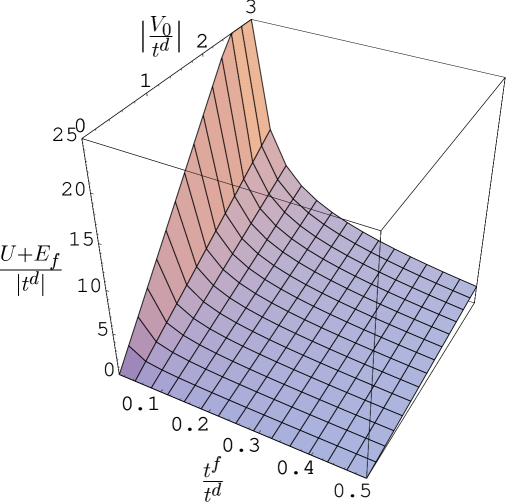
FIG. 5.: Phase diagram region where the localized solution occurs in the absence of next-nearest neighbor terms and isotropic case. The presented surface extends up to infinity for $(U+E_{f})/|t^{d}|\to\infty$.

REFERENCES

- [1] P. A. Lee et al. Comm.Cond.Matt.Phys. 12, 99, (1986).
- [2] Zs. Gulácsi, R. Starck, D. Vollhardt, Phys. Rev. B. 47, 8594, (1993).
- [3] M. A. N. Araujo, N. M. R. Peres, P. D. Sacramento, Phys. Rev. B. 65, 012503, (2001).
- [4] F. J. Ohkawa, Phys. Rev. B. 59, 8930, (1999).
- [5] E. H. Lieb, F. Y. Wu, Phys. Rev. Lett. 20, 1445, (1968).
- [6] U. Brandt, A. Giesekus, Phys. Rev. Lett. 68, 2648, (1992).
- [7] R. Strack, Phys. Rev. Lett. 70, 833, (1993).
- [8] I. Orlik, Zs. Gulácsi, Phil. Mag. B. 76, 845, (1997).
- [9] I. Orlik, Zs. Gulácsi, Phil. Mag. Lett. 78, 177, (1998).
- [10] T. Yanagisawa, Phys. Rev. Lett. 70, 2024, (1993).
- [11] C. Noce, A. Romano, C. Lubritto, Phys. Lett. A. 205, 313, (1995).
- [12] K. Ueda, H. Tsunetsugu, M. Sigrist, Phys. Rev. Lett. 68, 1030, (1992).
- [13] C. Noce, M. Cuoco, Phys. Rev. B. 54, 11951, (1996).
- [14] G. S. Tian, Phys. Rev. B. 50, 6246, (1994); and ibid. 63, 224413, (2001).
- [15] C. Noce, M. Cuoco, Phys. Rev. B. 59, 7409, (1999).
- [16] Zs. Gulacsi, I. Orlik, J. Phys. A.Lett. 34, L359, (2001).
- [17] I. Orlik, Zs. Gulácsi, Phil. Mag. B. 81, 1587, (2001).
- [18] P. Gurin, Zs. Gulacsi, Phys. Rev. B. 64, 045118, (2001).
- [19] B. Johansson, Phil. Mag. 30, 469, (1974).
- [20] K. Held, R. Bulla, Eur. Phys. J. B. 17, 7, (2000).
- [21] K. Held et al. Phys. Rev. Lett. 85, 373, (2000).
- [22] C. Huscroft, A. K. McMahan, R. T. Scalettar, Phys. Rev. Lett. 82, 2342, (1999).
- [23] K. Held, A. K. McMahan, R. T. Scalettar, Phys. Rev. Lett. 87, 276404, (2001).
- [24] M. B. Zölfl, I. A. Nekrasov, Th. Pruschke, V. I. Anisimov, J. Keller, Phys. Rev. Lett. 64, 276403, (2001).
- [25] P. van Dongen et al. Phys. Rev. B. 64,195123, (2001).
- [26] A. J. Arko et al., J. Elec. Spec. 117-118, 323, (2001).
- [27] R. Monnier, L. Degiorgi and D. D. Koelin, Phys. Rev. Lett. 56, 2744, (1986)
- [28] D. E. MacLaughlin, et al. Phys. Rev. Lett. 87, 066402, (2001).
- [29] S. R. Saha, H. Sugawara, T. Namiki, Y. Aoki, H. Sato, cond-mat/0206167.
- [30] R. B. Laughlin, G. G. Lonzarich, P. Monthoux, D. Pines, Advances in Phys. 50, 361, (2001).