SU(4) Skyrmions and Activation Energy Anomaly
in Bilayer Quantum Hall Systems

Abstract

The bilayer QH system has four energy levels in the lowest Landau level, corresponding to the layer and spin degrees of freedom. We investigate the system in the regime where all four levels are nearly degenerate and equally active. The underlying group structure is SU(4). At $\nu=1$ the QH state is a charge-transferable state between the two layers and the SU(4) isospin coherence develops spontaneously. Quasiparticles are isospin textures to be identified with SU(4) skyrmions. The skyrmion energy consists of the Coulomb energy, the Zeeman energy and the pseudo-Zeeman energy. The Coulomb energy consists of the self-energy, the capacitance energy and the exchange energy. At the balanced point only pseudospins are excited unless the tunneling gap is too large. Then, the SU(4) skyrmion evolves continuously from the pseudospin-skyrmion limit into the spin-skyrmion limit as the system is transformed from the balanced point to the monolayer point by controlling the bias voltage. Our theoretical result explains quite well the experimental data due to Murphy et al. and Sawada et al. on the activation energy anomaly induced by applying parallel magnetic field.

I Introduction

Exchange Coulomb interactions play key roles in various strongly correlated electron systems. They are essential also in quantum Hall (QH) systemsBookDasSarma ; BookEzawa , where spins are polarized spontaneously as in ferromagnets. Much more interesting phenomena occur in bilayer QH systems due to exchange interactions. For instance, an anomalous tunneling current has been observedSpielman00L between the two layers at the zero bias voltage. It may well be a manifestation of the Josephson-like phenomena predicted a decade agoEzawa92IJMPB . They occur due to quantum coherence developed spontaneously across the layersEzawa92IJMPB ; Ezawa97B ; Moon95B .

Electrons in a plane perform cyclotron motion under strong magnetic field $B_{\perp}$ and create Landau levels. When one Landau level is filled up the system becomes incompressible, leading to the integer QH effect. In QH systems the electron position is specified solely by the guiding center $\mathbf{X}=(X,Y)$ subject to the noncommutative relation, $[X,Y]=-i\ell_{B}^{2}$, with the magnetic length $\ell_{B}=\sqrt{\hbar/eB_{\perp}}$. The QH system provides us with a simple realization of noncommutative geometry. It follows from this relation that each electron occupies an area $2\pi\ell_{B}^{2}$ labelled by the Landau-site index. Electrons behave as if they were on lattice sites, among which exchange interactions operate.

In QH ferromagnets charged excitations are spin textures called skyrmionsSondhi93B . Skyrmions are identified experimentallyBarrett95L ; Aifer96L ; Schmeller95L by measuring the number of flipped spins per one quasiparticle. Indeed, by tilting samples, the activation energy increases by the Zeeman effect, which is roughly proportional to the number of flipped spins. On the contrary, an entirely opposite behavior has been observed by Murphy et al.Murphy94L in the bilayer QH system at the filling factor $\nu=1$, where the activation energy decreases rapidly by tilting samples. It is called the activation energy anomaly because of this unexpected behavior. Note that we expect an increase since the $\nu=1$ bilayer QH system is a QH ferromagnet with spins spontaneously polarized. This anomalous decrease has been argued to occur due to the loss of the exchange energy of a pseudospin texture based on the bimeron modelMoon95B , where the spin degree of freedom is frozen. Here, the layer degree of freedom is referred to as the pseudospin: It is said to be up (down) when an electron is in the front (back) layer.

We investigate physics taking place in the lowest Landau level (LLL). Since each Landau site can accommodate four electrons with the spin and layer degrees of freedom, the underlying group structure is enlarged to SU(4). Let us call it the isospin SU(4) in contrast to the spin SU(2) and the pseudospin SU(2). We study charged excitations in the $\nu=1$ bilayer QH system. A natural candidate is the SU(4) isospin texture to be identified with the SU(4) skyrmionEzawa99L ; BookEzawa . A specific feature of the SU(4) isospin texture is that it is reduced to the spin and pseudospin textures in certain limits.

At $\nu=1$, electrons are transferable between the two layers continuously without breaking the QH effectSawada97SSC . Namely, the bilayer QH system can be continuously brought into the monolayer QH system by changing the density imbalance. It implies that a pseudospin texture at the balanced point must be continuously transformed into a spin texture at the monolayer point. It is natural that a pseudospin texture evolves into an isospin texture and then regresses to a spin texture in this process. The corresponding continuous transformation of the activation energy has already been observed experimentally by Sawada et al.Sawada97SSC ; SawadaX03PE ; Terasawa04 . In this paper we explain these experimental dataMurphy94L ; SawadaX03PE ; Terasawa04 based on the excitation of SU(4) skyrmions.

In Section II we derive the Landau-site Hamiltonian governing bilayer QH systems, by extending the algebraic method employed previously to investigate multicomponent monolayer QH systemsEzawaX03B . In Section III we rewrite the Landau-site Hamiltonian into the exchange-interaction form. The Coulomb potentials associated with the direct and exchange interactions are obtained analytically.

In Section IV the ground state is explored in the regime where the SU(4) isospin coherence develops spontaneously. It is shown that the capacitance energy consists of two terms arising from the direct interaction, which is the standard one made of two planes, and from the exchange interaction, by way of which the capacitance energy becomes considerably smaller than the standard one for a small layer separation.

In Section V the excitation energy of an electron-hole pair is calculated exactly. A hole (electron) is the small size limit of a skyrmion (antiskyrmion), which is realized when the Zeeman gap $\Delta_{\text{Z}}$  and the tunneling gap $\Delta_{\text{SAS}}$ are very large. The exchange energy is very different whether the pair excites the spin or the pseudospin. Due to this difference the pseudospin excitation occurs at the balanced point even if the tunneling gap is quite large. Our result explains why pseudospin flips were observed in the experiment due to Terasawa et al.Terasawa04  in a sample having a very large tunneling gap ($\Delta_{\text{SAS}}\simeq 33$K). In Section VI we study skyrmions in a microscopic theory, extending the approachFertig94B previously known for the monolayer system.

In Section VII the effective Hamiltonian is derived from the Landau-site Hamiltonian by making the derivative expansion. We introduce composite bosons together with the CP³ fieldEzawa99L to describe coherent excitations. In Section VIII we carry out an analysis of SU(4) isospin textures identified with topological excitations called CP³ skyrmions or equivalently SU(4) skyrmions. A spin texture (spin-skyrmion) and a pseudospin texture (ppin-skyrmion) are special limits of an SU(4) skyrmion. We estimate the excitation energy of one SU(4) skyrmion. We show that, if a ppin-skyrmion is excited at the balanced point, it evolves continuously into a spin-skyrmion at the monolayer point via an SU(4) skyrmion as the density imbalance is increased between the two layers.

In Section IX we investigate the activation energy anomaly by applying the parallel magnetic field between the two layers. We calculate explicitly the loss of exchange energy of one SU(4) skyrmion, which is shown to be proportional to the capacitance term. Our theoretical result explains quite well both experimental data due to Murphy et al.Murphy94L and Sawada et al.SawadaX03PE ; Terasawa04 .

Section X is devoted to discussions.

II Landau-Site Hamiltonian

Electrons perform cyclotron motion under perpendicular magnetic field $B_{\bot}$. The number of flux quanta passing through the system is $N_{\Phi}\equiv B_{\perp}S/\Phi_{\text{D}}$, where $S$ is the area and $\Phi_{\text{D}}=2\pi\hbar/e$ is the flux quantum. There are $N_{\Phi}$ Landau sites per one Landau level, each of which is associated with one flux quantum and occupies an area $S/N_{\Phi}=2\pi\ell_{B}^{2}$. In the bilayer system an electron has two types of indices, the layer index (f, b) and the spin index ($\uparrow,\downarrow$). One Landau site may accommodate four electrons. The filling factor is $\nu=N/N_{\Phi}$ with $N$ the total number of electrons.

The kinetic Hamiltonian is

$$H_{\text{K}}={\frac{1}{2M}}\int\!d^{2}x\;\Psi^{{\dagger}}(\mathbf{x})(D_{x}-iD_{y})(D_{x}+iD_{y})\Psi(\mathbf{x}),$$ (1)

where $\Psi$ stands for the four-component electron field, and $D_{k}=-i\hbar\partial_{k}+eA_{k}$ is the covariant momentum. The kinetic Hamiltonian, which is invariant under the global SU(4) transformation, creates Landau levels. Assuming a large Landau level separation we focus on physics taking place in the LLL. Then we may neglect the kinetic energy since it is common to all states.

We introduce $4\times 4$ matrices $\tau_{a}^{\text{spin}}$ and $\tau_{a}^{\text{ppin}}$ generating the spin and pseudospin (ppin) SU(2) groups, as summarized in Appendix A; in particular, $\tau_{z}^{\text{spin}}=$diag$(1,-1,1,-1)$ and $\tau_{z}^{\text{ppin}}=$diag$(1,1,-1,-1)$. To avoid confusions we use $S_{a}$ for the spin SU(2) field, $P_{a}$ for the pseudospin SU(2) field ($a=x,y,z$) and $I_{A}$ for the isospin SU(4) field ($A=1,2,\cdots 15$).

The total Hamiltonian consists of the Coulomb term, the Zeeman term, the tunneling term and the bias term. The role of the bias term is to transfer electrons from one layer to the other by applying the bias voltage $V_{\text{bias}}$ between the two layers.

The Coulomb interaction is decomposed into the SU(4)-invariant and SU(4)-noninvariant terms,

$$H_{\text{C}}^{+} ={\frac{1}{2}}\int\!d^{2}xd^{2}y\;V^{+}(\mathbf{x}-\mathbf{y})\rho(\mathbf{x})\rho(\mathbf{y}),$$ (2)

$$H_{\text{C}}^{-} ={2}\int\!d^{2}xd^{2}y\;V^{-}(\mathbf{x}-\mathbf{y})P_{z}(\mathbf{x})P_{z}(\mathbf{y}),$$ (3)

where $\rho(\mathbf{x})=\Psi^{{\dagger}}(\mathbf{x})\Psi(\mathbf{x})$, $2P_{a}(\mathbf{x})=\Psi^{{\dagger}}(\mathbf{x})\tau_{a}^{\text{ppin}}\Psi(\mathbf{x})$ and

$$V^{\pm}(\mathbf{x})={\frac{e^{2}}{8\pi\varepsilon}}\left({\frac{1}{|\mathbf{x}|}\pm}\frac{1}{\sqrt{|\mathbf{x}|^{2}+d^{2}}}\right)$$ (4)

with the layer separation $d$.

The Zeeman term is

$$\mathcal{H}_{\text{Z}}=-\Delta_{\text{Z}}S_{z}(\mathbf{x),}$$ (5)

where $\Delta_{\text{Z}}$ is the Zeeman gap and $2S_{a}=\Psi^{{\dagger}}\tau_{a}^{\text{spin}}\Psi$. The tunneling and bias terms are combined into the pseudo-Zeeman term,

$$\mathcal{H}_{\text{PZ}}=-\Delta_{\text{SAS}}P_{x}(\mathbf{x})-eV_{\text{bias}}P_{z}(\mathbf{x}),$$ (6)

where $\Delta_{\text{SAS}}$ is the tunneling gap.

The total Hamiltonian is

$$H=H_{\text{C}}^{+}+H_{\text{C}}^{-}+H_{\text{Z}}+H_{\text{PZ}}.$$ (7)

We investigate the regime where the SU(4)-invariant Coulomb term $H_{\text{C}}^{+}$ dominates all other interactions. Note that the SU(4)-noninvariant Coulomb term vanishes, $H_{\text{C}}^{-}\rightarrow 0$, in the limit $d\rightarrow 0$.

We expand the electron field operator by a complete set of one-body wave functions $\varphi_{i}(\mathbf{x})=\langle\mathbf{x}|i\rangle$ in the LLL,

$$\psi_{\alpha}(\mathbf{x})\equiv\sum_{i=1}^{N_{\Phi}}c_{\alpha}(i)\varphi_{i}(\mathbf{x}),$$ (8)

where $c_{\alpha}(i)$ is the annihilation operator at the Landau site $|i\rangle$ with $\alpha=$f$\uparrow$, f$\downarrow$, b$\uparrow$ and b$\downarrow$,

$$\{c_{\alpha}(i),c_{\beta}^{\dagger}(j)\} =\delta_{ij}\delta_{\alpha\beta},$$

$$\{c_{\alpha}(i),c_{\beta}(j)\} =\{c_{\alpha}^{\dagger}(i),c_{\beta}^{\dagger}(j)\}=0.$$ (9)

It is impossible to choose an orthonormal complete set of one-body wave functions $\varphi_{i}(\mathbf{x})$ in the LLLIso92PLB . Hence $\psi_{\alpha}(\mathbf{x})$ does not satisfy the standard canonical anticommutation relation, as implies that an electron cannot be localized to a point within the LLL. Various interactions are projected to the LLLGirvin84B ; Iso92PLB ; Cappelli93NPB ; EzawaX03B by expanding the electron field as in (8).

The projected density is given by $\rho(\mathbf{x})=\Psi^{{\dagger}}(\mathbf{x})\Psi(\mathbf{x})$ with the use of the field operator (8). Its Fourier transformation readsEzawaX03B

$$\rho(\mathbf{q})={\frac{1}{2\pi}}e^{-\ell_{B}^{2}\mathbf{q}^{2}/4}\sum_{mn}\langle m|e^{-i\mathbf{qX}}|n\rangle c_{m}^{{\dagger}}c_{n},$$ (10)

where $\mathbf{X}=(X,Y)$ is the guiding center obeying the noncommutativity $[X,Y]=-i\ell_{B}^{2}$. Similar formulas hold for spin density operators and so on. Substituting them into (2) and (3) we find the projected Coulomb terms to be

$$H_{\text{C}}^{+}=\sum_{mnij}{V}_{mnij}^{+} \sum_{\alpha\beta}c_{\alpha}^{\dagger}(m)c_{\beta}^{\dagger}(i)c_{\beta}(j)c_{\alpha}(n),$$ (11)

$$H_{\text{C}}^{-}=\sum_{mnij}{V}_{mnij}^{-} \sum_{\alpha\beta\gamma\delta}[\tau_{z}^{\text{ppin}}]_{\alpha\beta}[\tau_{z}^{\text{ppin}}]_{\gamma\delta}$$

$$\times c_{\alpha}^{\dagger}(m)c_{\gamma}^{\dagger}(i)c_{\delta}(j)c_{\beta}(n)$$ (12)

with

$${V}_{mnij}^{\pm}={\frac{1}{4\pi}}\int d^{2}p\,V_{\text{D}}^{\pm}(\mathbf{p})\langle m|e^{i\mathbf{Xp}}|n\rangle\langle i|e^{-i\mathbf{Xp}}|j\rangle$$ (13)

and

$$V_{\text{D}}^{\pm}(\mathbf{p})=\frac{e^{2}}{8\pi\varepsilon}\frac{1\pm e^{-|\mathbf{p}|d}}{|\mathbf{p}|}e^{-\ell_{B}^{2}\mathbf{p}^{2}/2}.$$ (14)

We also find

$$H_{\text{Z}}= -\Delta_{\text{Z}}\sum_{m}S_{z}(m,m),$$ (15)

$$H_{\text{PZ}}= -\sum_{m}\left[\Delta_{\text{SAS}}P_{x}(m,m)+eV_{\text{bias}}P_{z}(m,m)\right],$$ (16)

where

$$\rho(m,n)= \sum_{\alpha}c_{\alpha}^{\dagger}(m)c_{\alpha}(n),$$

$$S_{a}(m,n)= \frac{1}{2}\sum_{\alpha\beta}c_{\alpha}^{\dagger}(m)[\tau_{a}^{\text{spin}}]_{\alpha\beta}c_{\beta}(n),$$ (17)

and a similar formula for $P_{a}(m,n)$. These formulas are derived precisely in the same way as for the multicomponent monolayer system with the replacement of the potential ${V}_{mnij}$ by ${V}_{mnij}^{+}$: See Section V in Ref.EzawaX03B .

For a later convenience we represent the projected Coulomb Hamiltonians (11) and (12) as

$$H_{\text{D}}^{+}= \sum_{mnij}{V}_{mnij}^{+}\rho(m,n)\rho(i,j),$$ (18)

$$H_{\text{D}}^{-}= 4\sum_{mnij}{V}_{mnij}^{-}P_{z}(m,n)P_{z}(i,j).$$ (19)

In the momentum space the total Coulomb Hamiltonian reads

$$H_{\text{D}}= \pi\int d^{2}p\,V_{\text{D}}^{+}(\mathbf{p})\widehat{\rho}(-\mathbf{p})\widehat{\rho}(\mathbf{p}),$$

$$+4\pi\int{\!}d^{2}p{\,}V_{\text{D}}^{-}(\mathbf{p})\widehat{P}_{z}(-\mathbf{p})\widehat{P}_{z}(\mathbf{p}),$$ (20)

where we have defined

$$\widehat{\rho}(\mathbf{p})= \frac{1}{2\pi}\sum_{mn}^{\infty}\langle m|e^{-i\mathbf{pX}}|n\rangle\rho(m,n),$$

$$\widehat{P}_{a}(\mathbf{p})= \frac{1}{2\pi}\sum_{mn}^{\infty}\langle m|e^{-i\mathbf{pX}}|n\rangle P_{a}(m,n).$$ (21)

We call (20) the direct-interaction form of the Coulomb Hamiltonian $\widehat{H}_{\text{C}}$.

Note the relation

$$\rho(\mathbf{q})=e^{-\ell_{B}^{2}\mathbf{q}^{2}/4}\widehat{\rho}(\mathbf{q}).$$ (22)

between the two types of densities (10) and (21). Though $\widehat{\rho}(\mathbf{p})$ presents a useful tool to work with noncommutative geometryEzawaX03B , it turns out that $\rho(\mathbf{q})$ describes the physical density [see (75)].

The density operator $\widehat{\rho}(\mathbf{p})$ satisfies the W_∞ algebraGirvin86B ; Iso92PLB ; Cappelli93NPB ,

$$[\widehat{\rho}(\mathbf{p}),\widehat{\rho}(\mathbf{q})]={\frac{i}{\pi}}\widehat{\rho}(\mathbf{p}+\mathbf{q})\sin\left[\frac{1}{2}\ell_{B}^{2}\mathbf{p}\!\wedge\!\mathbf{q}\right].$$ (23)

For the SU(4) isospin field we may define

$$I_{A}(m,n)=\frac{1}{2}\sum_{\alpha\beta}c_{\alpha}^{\dagger}(m)[\lambda_{A}]_{\alpha\beta}c_{\beta}(n),$$ (24)

where $\lambda_{A}$ is the generating matrices [See Appendix A], and

$$\widehat{I}_{A}(\mathbf{p})=\frac{1}{2\pi}\sum_{mn}^{\infty}\langle m|e^{-i\mathbf{pX}}|n\rangle I_{A}(m,n).$$ (25)

All of the density operators $\widehat{\rho}(\mathbf{p})$ and $\widehat{I}_{A}(\mathbf{p})$ form an algebra, which we have calledEzawaX03B W_∞(4) since it is the SU(4) extension of W_∞. It gives the fundamental algebraic structure of the noncommutative system made of 4-component electrons. In general there arises the W_∞(N) algebra in the N-component QH ferromagnet.

We define classical densities $\widehat{\rho}^{\text{cl}}(\mathbf{p})$, $\widehat{I}_{A}^{\text{cl}}(\mathbf{p})$, $\widehat{S}_{a}^{\text{cl}}(\mathbf{p})$ and $\widehat{P}_{a}^{\text{cl}}(\mathbf{p})$ by

$$\widehat{\rho}^{\text{cl}}(\mathbf{p})=\langle\mathfrak{S}|\widehat{\rho}(\mathbf{p})|\mathfrak{S}\rangle,\quad\widehat{I}_{A}^{\text{cl}}=\langle\mathfrak{S}|\widehat{I}_{A}(\mathbf{p})|\mathfrak{S}\rangle,$$ (26)

and so on, where $|\mathfrak{S}\rangle$ represents a skyrmion state. In the coordinate space the relation

$$\sum_{A=1}^{N^{2}-1}\widehat{I}_{A}^{\text{cl}}(\mathbf{x})\bigstar\widehat{I}_{A}^{\text{cl}}(\mathbf{x})=\frac{1}{2N}\widehat{\rho}^{\text{cl}}(\mathbf{x})\bigstar\left[\frac{N}{2\pi\ell_{B}^{2}}-\widehat{\rho}^{\text{cl}}(\mathbf{x})\right]$$ (27)

holds among the classical densities associated with the generators of the W_∞(N) algebra, where $\bigstar$ stands for the Moyal star product. We demonstrate this formula in Appendix B. Remark the invariance of (27) under

$$\hat{\rho}^{\text{cl}}(\mathbf{r})\rightarrow\frac{N}{2\pi\ell_{B}^{2}}-\hat{\rho}^{\text{cl}}(\mathbf{r}).$$ (28)

This represents the electron-hole symmetry.

III Exchange Interactions

In classical theory the Coulomb energy is simply given by (2) with the use of the classical density $\rho^{\text{cl}}(\mathbf{x})$, but this is not the case in quantum theory. The exchange interaction emerges as an important interaction from the exchange integral over wave functions. We present a rigorous treatment of the direct and exchange energies valid in QH systems.

For this purpose we rewrite the microscopic Coulomb Hamiltonians (11) and (12) into entirely different forms. Based on an algebraic relation,

$$\delta_{\sigma\beta}\delta_{\tau\alpha}=\frac{1}{2}\sum_{A}^{N^{2}-1}[\lambda_{A}]_{\sigma\tau}[\lambda_{A}]_{\alpha\beta}+\frac{1}{N}\delta_{\sigma\tau}\delta_{\alpha\beta},$$ (29)

which holds for SU(N) with $\lambda_{A}$ the generating matrices, these Coulomb Hamiltonians are equivalent to

$$H_{\text{X}}^{+}= -2\sum_{mnij}{V}_{mnij}^{+}\big{[}\sum_{A=1}^{15}I_{A}(m,j)I_{A}(i,n)$$

$$\hskip 57.81621pt+\frac{1}{2N}\rho(m,j)\rho(i,n)\big{]},$$ (30)

and

$$H_{\text{X}}^{-}= -2\sum_{mnij}V_{mnij}^{-}\big{[}\sum_{A=1}^{15}\xi_{A}I_{A}(m,j)I_{A}(i,n)$$

$$\hskip 57.81621pt+\frac{1}{2N}\rho(m,j)\rho(i,n)\big{]},$$ (31)

where $N=4$, $I_{A}(m,n)$ is defined by (24) and $\xi_{1,2,3,8,13,14,15}=+1$, $\xi_{4,5,6,7,9,10,11,12}=-1$. In the momentum space they read

$$H_{\text{X}}^{+}= \pi\int d^{2}p\,V_{\text{X}}^{+}(\mathbf{p})\big{[}\sum_{A=1}^{15}\widehat{I}_{A}(-\mathbf{p})\widehat{I}_{A}(\mathbf{p})$$

$$\hskip 72.26999pt+\frac{1}{2N}\widehat{\rho}(-\mathbf{p})\widehat{\rho}(\mathbf{p})\big{]},$$ (32)

$$H_{\text{X}}^{-}= 4\pi\int{\!}d^{2}p{\,}V_{\text{X}}^{-}(\mathbf{p})\big{[}\sum_{A=1}^{15}\xi_{A}\widehat{I}_{A}(-\mathbf{p})\widehat{I}_{A}(\mathbf{p})$$

$$\hskip 72.26999pt+\frac{1}{2N}\widehat{\rho}(-\mathbf{p})\widehat{\rho}(\mathbf{p})\big{]},$$ (33)

where

$$V_{\text{X}}^{\pm}(\mathbf{p})=\frac{\ell_{B}^{2}}{\pi}\int\!d^{2}k\,e^{-i\ell_{B}^{2}\mathbf{p}\wedge\mathbf{k}}V_{\text{D}}^{\pm}(\mathbf{k})$$ (34)

and $N=4$.

We change the SU(4) basis from $\lambda_{A}$ to $\tau_{a}^{\text{spin}}$, $\tau_{a}^{\text{ppin}}$ and $\tau_{a}^{\text{spin}}\tau_{b}^{\text{ppin}}$ by way of the formula (204) in Appendix, which transforms variable $I_{A}(m,n)$ to a set of variables,

$$S_{a}(m,n) =\frac{1}{2}\sum_{\sigma\tau}c_{\sigma}^{\dagger}(m)(\tau_{a}^{\text{spin}})_{\sigma\tau}c_{\tau}(n),$$

$$P_{a}(m,n) =\frac{1}{2}\sum_{\sigma\tau}c_{\sigma}^{\dagger}(m)(\tau_{a}^{\text{ppin}})_{\sigma\tau}c_{\tau}(n),$$

$$R_{ab}(m,n) =\frac{1}{2}\sum_{\sigma\tau}c_{\sigma}^{\dagger}(m)(\tau_{a}^{\text{spin}}\tau_{b}^{\text{ppin}})_{\sigma\tau}c_{\tau}(n).$$ (35)

The sum of (30) and (31) is expressed as

$$H_{\text{X}}= -\sum_{mnij}{V}_{mnij}^{d}[S_{a}(m,j)S_{a}(i,n)+P_{a}(m,j)P_{a}(i,n)$$

$$\hskip 57.81621pt+R_{ab}(m,j)R_{ab}(i,n)]$$

$$-2\sum_{mnij}V_{mnij}^{-}[S_{a}(m,j)S_{a}(i,n)+P_{z}(m,j)P_{z}(i,n)$$

$$\hskip 57.81621pt+R_{az}(m,j)R_{az}(i,n)]$$

$$-\frac{1}{4}\sum_{mnij}{V}_{mnij}\rho(m,j)\rho(i,n),$$ (36)

where

$${V}_{mnij}={V}_{mnij}^{+}+{V}_{mnij}^{-},\quad{V}_{mnij}^{d}={V}_{mnij}^{+}-{V}_{mnij}^{-}.$$ (37)

In the momentum space we find

$$H_{\text{X}}= -\frac{\pi}{2}\int{\!}d^{2}p\,V_{\text{X}}^{d}(\mathbf{p})[\widehat{S}_{a}(-\mathbf{p})\widehat{S}_{a}(\mathbf{p})+\widehat{P}_{a}(-\mathbf{p})\widehat{P}_{a}(\mathbf{p})$$

$$\hskip 57.81621pt+\widehat{R}_{ab}(-\mathbf{p})\widehat{R}_{ab}(\mathbf{p})]$$

$$-\pi\int{\!}d^{2}p\,V_{\text{X}}^{-}(\mathbf{p})[\widehat{S}_{a}(-\mathbf{p})\widehat{S}_{a}(\mathbf{p})+\widehat{P}_{z}(-\mathbf{p})\widehat{P}_{z}(\mathbf{p})$$

$$\hskip 57.81621pt+\widehat{R}_{az}(-\mathbf{p})\widehat{R}_{az}(\mathbf{p})]$$

$$-\frac{\pi}{8}\int{\!}d^{2}p{\,}V_{\text{X}}(\mathbf{p})\widehat{\rho}(-\mathbf{p})\widehat{\rho}(\mathbf{p}),$$ (38)

where

$$V_{\text{X}}(\mathbf{p})=V_{\text{X}}^{+}(\mathbf{p})+V_{\text{X}}^{-}(\mathbf{p}),\quad V_{\text{X}}^{d}(\mathbf{p})=V_{\text{X}}^{+}(\mathbf{p})-V_{\text{X}}^{-}(\mathbf{p}).$$ (39)

In (36) and (38) the summation ($\sum_{a=xyz}$,$\sum_{b=xyz}$) over the repeated indices $a$ and $b$ is understood. We call (38) the exchange-interaction form of the Coulomb Hamiltonian $\widehat{H}_{\text{C}}$.

We have demonstrated that the Landau-site Hamiltonian $H_{\text{C}}$ possesses two entirely different forms, the direct-interaction form $H_{\text{D}}$ given by (20) and the exchange-interaction form $H_{\text{X}}$ given by (38). They are equivalent, $H_{\text{D}}=H_{\text{X}}$, as the microscopic Hamiltonian. In this paper we are interested in the excitation energy $\langle\mathfrak{S}|H|\mathfrak{S}\rangle$ of a skyrmion state $|\mathfrak{S}\rangle$. In a previous paperEzawaX03B we have presented a heuristic argument showing that

$$\langle\mathfrak{S}|H_{\text{C}}|\mathfrak{S}\rangle=H_{\text{D}}^{\text{cl}}+H_{\text{X}}^{\text{cl}}.$$ (40)

Here $H_{\text{D}}^{\text{cl}}$ and $H_{\text{X}}^{\text{cl}}$ are the Hamiltonians of the direct-interaction form (20) and of the exchange-interaction form (38), where the density operators $\widehat{\rho}(\mathbf{p})$, $\widehat{I}_{A}(\mathbf{p})$, $\cdots$ are replaced by the classical ones $\widehat{\rho}^{\text{cl}}(\mathbf{p})$, $\widehat{I}_{A}^{\text{cl}}(\mathbf{p})$, $\cdots$. We present a proof of this formula for the skyrmion state in Appendix B. Thus, the energy of a charge excitation consists of two well-separated pieces, the direct energy and the exchange energy.

IV Ground State

We first determine the ground state of the bilayer system in this section. For simplicity we start with the spin-frozen SU(2) bilayer system. We are concerned about the regime dominated by the SU(2)-invariant Coulomb interaction $H_{\text{C}}^{+}$. Hence we define the ground state as an eigenstate of $H_{\text{C}}^{+}$ given by (11), and treat all other interactions as small perturbations.

The unperturbed ground-state energy is given by

$$H_{\text{C}}^{+}|\text{g}\rangle=\sum_{jn}V_{jnnj}^{+}|\text{g}\rangle=-\epsilon_{\text{X}}^{+}N_{\Phi}|\text{g}\rangle$$ (41)

with

$$\epsilon_{\text{X}}^{\pm}= \frac{1}{N_{\Phi}}\sum_{jn}V_{jnnj}^{\pm}={\frac{1}{4\pi}}\int d^{2}k\,V_{\text{D}}^{\pm}(\mathbf{k})$$

$$= \frac{1}{2}\left[1\pm e^{d^{2}/2\ell_{B}^{2}}\text{erfc}\left(d/\sqrt{2}\ell_{B}\right)\right]\Delta_{\text{C}}^{0},$$ (42)

where

$$\Delta_{\text{C}}^{0}=\frac{1}{2}\sqrt{\frac{\pi}{2}}\frac{e^{2}}{4\pi\varepsilon\ell_{B}}.$$ (43)

We take $\Delta_{\text{C}}^{0}$ as the Coulomb energy unit in this paper. The unperturbed system is equivalent to the monolayer SU(2) QH ferromagnet, where all pseudospins are spontaneously polarized into one arbitrary direction in the SU(2) pseudospin space. The ground state may be expressed as

$$|\text{g}\rangle=\prod_{n} \left\{e^{i\vartheta_{0}/2}\sqrt{{\frac{1+\sigma_{0}}{2}}}c_{\text{f}}^{\dagger}(n)\right.$$

$$\left.+e^{-i\vartheta_{0}/2}\sqrt{{\frac{1-\sigma_{0}}{2}}}c_{\text{b}}^{\dagger}(n)\right\}|0\rangle,$$ (44)

by introducing two constant parameters $\sigma_{0}$ and $\vartheta_{0}$. We call $\sigma_{0}$ the imbalance parameter since it represents the density imbalance between the two layers. The ground state is a coherent state due to an infinite degeneracy with respect to $\sigma_{0}$ and $\vartheta_{0}$.

We then study the effect due to the SU(2)-noninvariant interaction. First, due to the capacitance effect ($\varpropto V_{mnij}^{-}$) all pseudospins are polarized into one arbitrary direction within the pseudospin $xy$ plane, implying that the electron density is balanced between the two layers ($\sigma_{0}=0$). The symmetry SU(2) is broken into U(1). It is thus said that the bilayer QH system is an easy plane ferromagnet. Next, we apply the bias voltage to generate an imbalanced density state ($\sigma_{0}\neq 0$), where the symmetry is still U(1). Finally, the tunneling interaction breaks the symmetry completely by fixing $\vartheta_{0}=0$ in the state (44). Consequently, the ground state is the bonding state $|$B$\rangle$ parametrized by the imbalance parameter $\sigma_{0}$, which is (44) with $\vartheta_{0}=0$.

The generalization to the SU(4) bilayer system is trivial by adding the spin component. The ground state turns out to be the up-spin bonding state $|$B$\uparrow\rangle$ due to the Zeeman effect. It is convenient to represent the up-spin bonding state $|$B$\uparrow\rangle$ and the up-spin antibonding state $|$A$\uparrow\rangle$ as

$$|\text{B\negthinspace}\uparrow\rangle=\prod\limits_{n}B_{\uparrow}^{\dagger}(n)|0\rangle,\quad|\text{A\negthinspace}\uparrow\rangle=\prod\limits_{n}A_{\uparrow}^{\dagger}(n)|0\rangle,$$ (45)

where

$$\left(\begin{array}[]{c}B_{\uparrow}(n)\\ A_{\uparrow}(n)\end{array}\right)={\frac{1}{\sqrt{2}}}\left(\begin{array}[]{@{\,}rr}\sqrt{1+\sigma_{0}}&\sqrt{1-\sigma_{0}}\\ \sqrt{1-\sigma_{0}}&-\sqrt{1+\sigma_{0}}\end{array}\right)\left(\begin{array}[]{c}c_{\text{f}\uparrow}(n)\\ c_{\text{b}\uparrow}(n)\end{array}\right).$$ (46)

The down-spin bonding state $|$B$\downarrow\rangle$ and the down-spin antibonding state $|$A$\downarrow\rangle$ are similarly defined.

We evaluate the ground state energy $E_{\text{g}}=\langle B\!\!\uparrow|H|B\!\!\uparrow\rangle$ by representing the Hamiltonians in terms of these operator. The ground-state energy per one site reads

$$E_{\text{g}}/N_{\Phi} =-\epsilon_{\text{X}}^{+}+\frac{1}{4}\epsilon_{\text{cap}}\sigma_{0}^{2}$$

$$-\frac{1}{2}\Delta_{\text{SAS}}\sqrt{1-\sigma_{0}^{2}}-\frac{1}{2}eV_{\text{bias}}\sigma_{0}-\Delta_{\text{Z}},$$ (47)

where

$$\epsilon_{\text{cap}}=4(\epsilon_{\text{D}}^{-}-\epsilon_{\text{X}}^{-})$$ (48)

with

$$\epsilon_{\text{D}}^{-}=\frac{1}{N_{\Phi}}\sum_{jn}{V}_{nnjj}^{-}=\sqrt{\frac{1}{2\pi}}\frac{d}{\ell_{B}}\Delta_{\text{C}}^{0},$$ (49)

and $\epsilon_{\text{X}}^{-}$ given by (42). The imbalance parameter $\sigma_{0}$ is determined to minimize the ground-state energy,

$$\epsilon_{\text{cap}}\sigma_{0}+{\frac{\Delta_{\text{SAS}}\sigma_{0}}{\sqrt{1-\sigma_{0}^{2}}}}=eV_{\text{bias}},$$ (50)

as a function of the bias voltage.

The second term in the ground-state energy (47) is the capacitance energy,

$$E_{\text{g}}^{\text{cap}}=\frac{\epsilon_{\text{cap}}\sigma_{0}^{2}}{4}N_{\Phi}\equiv{\frac{Q^{2}}{2C}S,}$$ (51)

where $Q={\frac{1}{2}e}\rho_{0}\sigma_{0}$ is the charge imbalance and $C$ is the capacitance per unit area. We rewrite (50) as

$${\frac{Q}{C}}+V_{\text{junc}}=V_{\text{bias}},$$ (52)

with

$$eV_{\text{junc}}={\frac{\sigma_{0}}{\sqrt{1-\sigma_{0}^{2}}}}\Delta_{\text{SAS}}.$$ (53)

When the tunneling interaction is absent ($\Delta_{\text{SAS}}\rightarrow 0$), (52) is reduced to

$$Q=CV_{\text{bias}}.$$ (54)

Eqs. (51) and (54) are the well-known formulas for the condenser, where the bias voltage $V_{\text{bias}}$ is balanced with the electric potential $Q/C$ due to the charge difference $Q$ between the two layers. In this case, a charge transfer between the two layers makes no work, since there exists no potential difference between the two layers.

When $\Delta_{\text{SAS}}\neq 0$, the cancellation is imperfect as in (52). Thus, when a charge is moved from one layer to the other, it is necessary to supply an energy against the potential difference $V_{\text{junc}}=V_{\text{bias}}-Q/C$. Consequently, the pseudo-Zeeman energy is given by

$$\mathcal{H}_{\text{PZ}} =-\left[\Delta_{\text{SAS}}P_{x}(\mathbf{x})+eV_{\text{junc}}P_{z}(\mathbf{x})\right]$$

$$=-\left[P_{x}(\mathbf{x})+\frac{\sigma_{0}}{\sqrt{1-\sigma_{0}^{2}}}P_{z}(\mathbf{x})\right]\Delta_{\text{SAS}},$$ (55)

or

$$H_{\text{PZ}}=-\sum_{m}\left[P_{x}(m,m)+\frac{\sigma_{0}}{\sqrt{1-\sigma_{0}^{2}}}P_{z}(m,m)\right]\Delta_{\text{SAS}}.$$ (56)

As $\Delta_{\text{SAS}}\rightarrow 0$, the pseudo-Zeeman energy vanishes even in imbalanced configuration ($\sigma_{0}\neq 0$), and the total ground-state energy consists solely of the capacitance energy (51). In order to analyze charge excitations it is necessary to use (56) as the pseudo-Zeeman term in the total Hamiltonian (7).

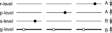
Figure 1: The LLL contains four energy levels corresponding to the two layers and the two spin states. (We call them the g-level, s-level, p-level and r-level.) At $\nu=1$ the ground state is the up-spin bonding state. An electron may be moved to any one of the other three levels to form an electron-hole pair excitation.

V Electron and Hole Excitations

As we see in the succeeding section, a skyrmion and an antiskyrmion are reduced to a hole and an electron in their small size limit. We analyze electron and hole excitations in this section to derive some exact results.

V.1 Electron-Hole Pair Excitation

One electron may be excited from the up-spin bonding state into the down-spin bonding state, the up-spin antibonding state or the down-spin antibonding state [FIG.1]. These electron-hole states are

$$|\psi_{\text{s}}\rangle=|\text{e}_{j}^{\text{B}\downarrow};\text{h}_{k}^{\text{B}\uparrow}\rangle=B_{\downarrow}^{{\dagger}}(j)B_{\uparrow}(k)|\text{B\negthinspace\negthinspace}\uparrow\rangle,$$ (57)

$$|\psi_{\text{p}}\rangle=|\text{e}_{j}^{\text{A}\uparrow};\text{h}_{k}^{\text{B}\uparrow}\rangle=A_{\uparrow}^{{\dagger}}(j)B_{\uparrow}(k)|\text{B\negthinspace\negthinspace}\uparrow\rangle,$$ (58)

$$|\psi_{\text{r}}\rangle=|\text{e}_{j}^{\text{A}\downarrow};\text{h}_{k}^{\text{B}\uparrow}\rangle=A_{\downarrow}^{{\dagger}}(j)B_{\uparrow}(k)|\text{B\negthinspace\negthinspace}\uparrow\rangle.$$ (59)

We assume that an electron and a hole are separated far enough so that interactions between them are neglected. The energy matrix looks as

$$\left(\begin{array}[]{ccc}\langle\psi_{\text{s}}|H|\psi_{\text{s}}\rangle&\langle\psi_{\text{s}}|H|\psi_{\text{r}}\rangle&0\\ \langle\psi_{\text{r}}|H|\psi_{\text{s}}\rangle&\langle\psi_{\text{r}}|H|\psi_{\text{r}}\rangle&0\\ 0&0&\langle\psi_{\text{p}}|H|\psi_{\text{p}}\rangle\end{array}\right),$$ (60)

where

$$\langle\psi_{\text{s}}|H|\psi_{\text{s}}\rangle= E_{\text{g}}+2\epsilon_{\text{X}}^{+}+2\sigma_{0}^{2}\epsilon_{\text{X}}^{-}+\Delta_{\text{Z}},$$

$$\langle\psi_{\text{r}}|H|\psi_{\text{r}}\rangle= E_{\text{g}}+2\epsilon_{\text{X}}^{+}-2\sigma_{0}^{2}\epsilon_{\text{X}}^{-}-\sigma_{0}^{2}\epsilon_{\text{cap}}+\Delta_{\text{Z}}+\frac{\Delta_{\text{SAS}}}{\sqrt{1-\sigma_{0}^{2}}},$$

$$\langle\psi_{\text{p}}|H|\psi_{\text{p}}\rangle= E_{\text{g}}+2\epsilon_{\text{X}}^{+}-2\epsilon_{\text{X}}^{-}-\sigma_{0}^{2}\epsilon_{\text{cap}}+\frac{\Delta_{\text{SAS}}}{\sqrt{1-\sigma_{0}^{2}}},$$

$$\langle\psi_{\text{r}}|H|\psi_{\text{s}}\rangle= 2\sigma_{0}\sqrt{1-\sigma_{0}^{2}}\epsilon_{\text{D}}^{-}.$$ (61)

We have $\langle\psi_{\text{s}}|H|\psi_{\text{p}}\rangle=\langle\psi_{\text{r}}|H|\psi_{\text{p}}\rangle=0$, because the Hamiltonian does not flip the spin (it does not involve $S_{x}$ and $S_{y}$).

The matrix (60) is diagonal at the balanced point. The minimum eigenvalue is the spin-excitation energy

$$\langle\psi_{\text{s}}|H|\psi_{\text{s}}\rangle=E_{\text{g}}+2\epsilon_{\text{X}}^{+}+\Delta_{\text{Z}},$$ (62)

or the ppin excitation energy

$$\langle\psi_{\text{p}}|H|\psi_{\text{p}}\rangle=E_{\text{g}}+2\epsilon_{\text{X}}^{+}-2\epsilon_{\text{X}}^{-}+\Delta_{\text{SAS}}.$$ (63)

The pseudospin excitation occurs when

$$2\epsilon_{\text{X}}^{-}>\Delta_{\text{SAS}}-\Delta_{\text{Z}}.$$ (64)

We remark that $2\epsilon_{\text{X}}^{-}\simeq 47$K in a typical sample with $d\simeq 231$ nm.

The matrix (60) is diagonal also at the monolayer point, where the spin excitation always occurs with the excitation energy

$$\langle\psi_{\text{s}}|H|\psi_{\text{s}}\rangle=E_{\text{g}}+2\left(\epsilon_{\text{X}}^{+}+\epsilon_{\text{X}}^{-}\right)+\Delta_{\text{Z}},$$ (65)

since the energies of the other two modes diverge.

The two excitation states $|\psi_{\text{s}}\rangle$ and $|\psi_{\text{r}}\rangle$ mix to make a new state, $|\psi_{\text{sr}}\rangle$, to lower the excitation energy except for $\sigma_{0}=0$ and $\sigma_{0}=1$. After diagonalization it is

$$\langle\psi_{\text{sr}}| H|\psi_{\text{sr}}\rangle=E_{\text{g}}+2\epsilon_{\text{X}}^{+}-\frac{1}{2}\sigma_{0}^{2}\epsilon_{\text{cap}}+\Delta_{\text{Z}}+\frac{1}{2}\widetilde{\Delta}_{\text{SAS}}$$

$$-\frac{1}{2}\sqrt{(\widetilde{\Delta}_{\text{SAS}}-4\sigma_{0}^{2}\epsilon_{\text{D}}^{-})^{2}+16\sigma_{0}^{2}(1-\sigma_{0}^{2})(\epsilon_{\text{D}}^{-})^{2}}$$ (66)

with $\widetilde{\Delta}_{\text{SAS}}=\Delta_{\text{SAS}}/\sqrt{1-\sigma_{0}^{2}}$. Thus, when the condition (64) is satisfied, an electron is excited to the $|\psi_{\text{p}}\rangle$ state at the balanced point, and it makes a sudden transition to the $|\psi_{\text{sr}}\rangle$ state, and finally transforms smoothly into the $|\psi_{\text{s}}\rangle$ state, as depicted in FIG.2. The sudden transition would be smoothed out in a skyrmion-antiskyrmion excitation involving several electrons simultaneously.

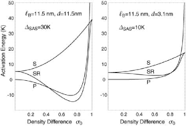
Figure 2: The energy of an electron-hole pair state is depicted as a function of the imbalance parameter $\sigma_{0}$ based on the formulas ( 61) and (66) with typical sample parameters as indicated. Three curves corresponds to the state $|\psi_{\text{s}}\rangle$, $|\psi_{\text{sr}}\rangle$ and $|\psi_{\text{p}}\rangle$. We have normalized the activation energy of the pseudospin excitation to zero at $\sigma_{0}=0$.

V.2 Physical Densities

It is interesting to investigate a single electron excitation and a single hole excitation separately. For simplicity we analyze the SU(2) QH ferromagnet. One-electron excited state $|\mathfrak{S}_{+}\rangle$ and one-hole excited state $|\mathfrak{S}_{-}\rangle$ are given by

$$|\mathfrak{S}_{+}\rangle=c_{\downarrow}^{\dagger}(0)\prod_{n}c_{\uparrow}^{\dagger}(n)|0\rangle,\mathbf{\quad}|\mathfrak{S}_{-}\rangle=\prod_{n\neq 0}c_{\uparrow}^{\dagger}(n)|0\rangle,$$ (67)

where we have placed an electron or a hole at the momentum-zero state. Their classical densities are

$$\rho_{\pm}^{\text{cl}}(m,n)= \sum_{\sigma}\langle\mathfrak{S}_{\pm}|c_{\sigma}^{\dagger}(m)c_{\sigma}(n)|\mathfrak{S}_{\pm}\rangle$$

$$= \delta_{mn}\pm\delta_{m0}\delta_{n0}.$$ (68)

In the coordinate space, based on formula (21) it reads

$$\widehat{\rho}_{\pm}^{\text{cl}}(\mathbf{x})=\rho_{0}\left(1\pm 2e^{-r^{2}/\ell_{B}^{2}}\right),$$ (69)

where $\rho_{0}$ is the electron density in the ground state. The hole density becomes negative at the origin,

$$\lim_{\mathbf{x}\rightarrow 0}\widehat{\rho}_{-}^{\text{cl}}(\mathbf{x})=-\rho_{0}.$$ (70)

There is nothing wrong with this mathematically since the electron cannot be localized within the LLL. Nevertheless, we cannot accept this as a physical quantity.

We recall that the wave function of one electron with the angular-momentum zero in the LLL is

$$\varphi_{0}(\mathbf{x})=\frac{1}{\sqrt{2\pi\ell_{B}^{2}}}e^{-r^{2}/4\ell_{B}^{2}},$$ (71)

which leads to the density

$$\delta\rho^{\text{cl}}(\mathbf{x})=|\varphi_{0}(\mathbf{x})|^{2}=\rho_{0}e^{-r^{2}/2\ell_{B}^{2}}$$ (72)

at $\nu=2\pi\ell_{B}^{2}\rho_{0}=1$. When we remove one electron from or add one electron to the filled up-spin level, the density becomes

$$\rho_{\pm}^{\text{cl}}(\mathbf{x})=\rho_{0}\pm\delta\rho^{\text{cl}}(\mathbf{x}),$$ (73)

and the hole density satisfies

$$\lim_{\mathbf{x}\rightarrow 0}\rho_{-}^{\text{cl}}(\mathbf{x})=0.$$ (74)

This behavior is what we expect for the physical density at the origin.

It is easy to see that the Fourier transformations of (69) and (73) are related as

$$\rho_{\text{h}}^{\text{cl}}(\mathbf{q})=e^{-\ell_{B}^{2}\mathbf{q}^{2}/4}\widehat{\rho}_{\text{h}}^{\text{cl}}(\mathbf{q}).$$ (75)

This is precisely the relation (22) between the two types of the densities. We conclude that the projected density represents a physical quantity.

V.3 Direct and Exchange Energies

For simplicity we work still in the SU(2) QH ferromagnet. The electron-hole pair excitation energy isKallin91B

$$\delta E_{\text{pair}}=\langle\psi_{\text{s}}|H_{\text{C}}|\psi_{\text{s}}\rangle-E_{\text{g}}=2\epsilon_{\text{X}},$$ (76)

where

$$\epsilon_{\text{X}}={V}_{0000}+\sum_{j\neq 0}V_{j00j}=\Delta_{\text{C}}^{0},$$ (77)

as is obtained by taking $d\rightarrow 0$ in (42) and (61). It follows from (13) that ${V}_{0000}$ is the direct integral and $V_{j00j}$ ($j\neq 0$) is the exchange integral. Hence, the Coulomb energy consists of the direct energy $\delta H_{\text{D}}^{\text{cl}}={V}_{0000}$ and the exchange energy $\delta H_{\text{X}}^{\text{cl}}=\sum_{j\neq 0}V_{j00j}$.

We can express them in familiar forms. First, the classical energy associated with the density modulation (68) reads

$$\delta H_{\text{D}}^{\text{cl}}=\sum_{mnij}{V}_{mnij}\delta\rho^{\text{cl}}(m,n)\delta\rho^{\text{cl}}(i,j)={V}_{0000}$$ (78)

with $\delta\rho^{\text{cl}}(m,n)=\delta_{m0}\delta_{n0}$, which is transformed into

$$\delta H_{\text{D}}^{\text{cl}}={\frac{1}{2}}\int\!d^{2}xd^{2}y\;V(\mathbf{x}-\mathbf{y})\delta\rho^{\text{cl}}(\mathbf{x})\delta\rho^{\text{cl}}(\mathbf{y})$$ (79)

with $\delta\rho^{\text{cl}}(\mathbf{x})$ being given by (72). This is the direct energy of the excitation. We next remark that the spin reads

$$S_{x}^{\text{cl}}(m,n)= S_{y}^{\text{cl}}(m,n)=0,$$

$$S_{z}^{\text{cl}}(m,n)= \frac{1}{2}\left(\delta_{mn}-\delta_{m0}\delta_{n0}\right)$$ (80)

both for the electron or hole excitation. Substituting them into the exchange energy (30), or

$$H_{\text{X}}^{\text{cl}}= -2\sum_{mnij}{V}_{mnij}\big{[}\sum_{a=xyz}S_{a}^{\text{cl}}(m,j)S_{a}^{\text{cl}}(i,n)$$

$$\hskip 57.81621pt+\frac{1}{4}\rho_{\pm}^{\text{cl}}(m,j)\rho_{\pm}^{\text{cl}}(i,n)\big{]},$$ (81)

we reproduce $\delta H_{\text{X}}^{\text{cl}}=\sum_{j\neq 0}V_{j00j}$. In the momentum space we have a more familiar expression,

$$H_{\text{X}}^{\text{cl}}= \pi\int d^{2}p\,V_{\text{X}}(\mathbf{p})\big{[}\sum_{a=xyz}\widehat{S}_{a}^{\text{cl}}(-\mathbf{p})\widehat{S}_{a}^{\text{cl}}(\mathbf{p})$$

$$\hskip 57.81621pt+\frac{1}{4}\widehat{\rho}^{\text{cl}}(-\mathbf{p})\widehat{\rho}^{\text{cl}}(\mathbf{p})\big{]}.$$ (82)

Thus, the excitation energy of an electron or a hole presents us the simplest example of the decomposition formula (40) into the direct and exchange energies.

VI Skyrmions in Microscopic Theory

We study skyrmions in a microscopic theory of the SU(2) QH ferromagnet, and then extend the scheme to the SU(4) bilayer QH ferromagnet. We set $\ell_{B}=1$ throughout in this section, where $\rho_{0}=1/2\pi$.

VI.1 SU(2) Skyrmions

A skyrmion and an antiskyrmion are topological solitons in the nonlinear sigma model, and characterized by the nonlinear sigma field (normalized spin field),

$$\mathcal{S}_{x}=\frac{\alpha x}{r^{2}+\alpha^{2}},\quad\mathcal{S}_{y}=\frac{\mp\alpha y}{r^{2}+\alpha^{2}},\quad\mathcal{S}_{z}=\frac{1}{2}-\frac{\alpha^{2}}{r^{2}+\alpha^{2}},$$ (83)

when it carries topological charge $\pm 1$. Actual skyrmions are much more complicated in the QH ferromagnet because the spin rotation modulates the electron density due to the W_∞(2) algebra. Nevertheless, a gross feature remains as it isBookEzawa .

Let $|\mathfrak{S}\rangle$ be the skyrmion state. Its spin field is given by [see (21)]

$$\widehat{S}_{a}^{\text{cl}}(\mathbf{p})=\frac{1}{2\pi}\sum_{mn}^{\infty}\langle m|e^{-i\mathbf{pX}}|n\rangle\langle\mathfrak{S}|S_{a}(m,n)|\mathfrak{S}\rangle.$$ (84)

Due to the formula

$$\langle m| e^{i\mathbf{kX}}|m+n\rangle$$

$$=\frac{\sqrt{m!}}{\sqrt{(m+n)!}}\left(\frac{k_{y}+ik_{x}}{\sqrt{2}}\right)^{n}e^{-\mathbf{k}^{2}/4}L_{m}^{n}\left(\frac{\mathbf{k}^{2}}{2}\right),$$ (85)

we need to have $\langle\mathfrak{S}|S_{x,y}(m,n)|\mathfrak{S}\rangle\varpropto\delta_{m,n\pm 1}$ and $\langle\mathfrak{S}|S_{z}(m,n)|\mathfrak{S}\rangle\varpropto\delta_{m,n}$ to be consistent with (83). Such a state is uniquely constructed asFertig94B

$$|\mathfrak{S}_{\text{sky}}\rangle=\prod_{n=0}\xi^{\dagger}(n)|0\rangle$$ (86)

with

$$\xi^{\dagger}(n)=u(n)c_{\downarrow}^{\dagger}(n)+v(n)c_{\uparrow}^{\dagger}(n+1).$$ (87)

They satisfy the standard canonical commutation relations,

$$[\xi(m),\xi^{\dagger}(n)]=\delta_{mn},\quad[\xi(m),\xi(n)]=0,$$ (88)

provided $u^{2}(n)+v^{2}(n)=1$. Note the state $|\mathfrak{S}_{\text{sky}}\rangle$ describes one hole state in the momentum-zero site when we set $u(n)=0$ and $v(n)=1$ for all $n$.

Similarly, the antiskymion state is given byFertig94B

$$|\mathfrak{S}_{\text{asky}}\rangle=\prod_{n=0}\zeta^{\dagger}(n)c_{\downarrow}^{\dagger}(0)|0\rangle$$ (89)

with

$$\zeta^{\dagger}(n)=-u(n)c_{\downarrow}^{\dagger}(n+1)+v(n)c_{\uparrow}^{\dagger}(n).$$ (90)

The state $|\mathfrak{S}_{\text{asky}}\rangle$ describes one electron excited state in the momentum-zero site when we set $u(n)=0$ and $v(n)=1$ for all $n$. In what follow we only discuss the skyrmion case explicitly.

First we evaluate $\widehat{\rho}^{\text{cl}}(m,n)=\langle\mathfrak{S}|\rho(m,n)|\mathfrak{S}\rangle$ and others. The only nonvanishing components are [see (213) in Appendix B]

$$\widehat{\rho}^{\text{cl}}(m,m) =u^{2}(m)+v^{2}(m-1),$$

$$\widehat{S}_{z}^{\text{cl}}(m,m) =-\frac{1}{2}\left[u^{2}(m)-v^{2}(m-1)\right],$$

$$\widehat{S}_{x}^{\text{cl}}(m,m+1) =\widehat{S}_{x}^{\text{cl}}(m+1,m)=-i\widehat{S}_{y}^{\text{cl}}(m,m+1)$$

$$=i\widehat{S}_{y}^{\text{cl}}(m+1,m)=\frac{1}{2}u(m)v(m),$$ (91)

where we have set $v(-1)=0$. They are converted into the momentum space based on the formula (21),

$$\widehat{\rho}^{\text{cl}}(\mathbf{k})= \frac{1}{2\pi}e^{-k^{2}/4}\sum_{m=0}\left[u^{2}(m)+v^{2}(m-1)\right]L_{m}\left(k^{2}/2\right),$$

$$\widehat{S}_{z}^{\text{cl}}(\mathbf{k})= -\frac{1}{4\pi}e^{-k^{2}/4}\sum_{m=0}\left[u^{2}(m)-v^{2}(m-1)\right]L_{m}\left(k^{2}/2\right),$$

$$\widehat{S}_{x}^{\text{cl}}(\mathbf{k})= \frac{-ik_{a}}{2\sqrt{2}\pi}e^{-k^{2}/4}\sum_{m=0}\frac{u(m)v(m)}{\sqrt{m+1}}L_{m}^{(1)}\left(k^{2}/2\right),$$

$$\widehat{S}_{y}^{\text{cl}}(\mathbf{k})= \frac{ik_{a}}{2\sqrt{2}\pi}e^{-k^{2}/4}\sum_{m=0}\frac{u(m)v(m)}{\sqrt{m+1}}L_{m}^{(1)}\left(k^{2}/2\right)$$ (92)

after some calculation with the use of (85).

The electron number defference between the skyrmion state and the ground state is

$$\delta Q= \sum_{m=0}^{\infty}[\widehat{\rho}^{\text{cl}}(m,m)-1]$$

$$= u^{2}(0)-1+\sum_{m=1}^{\infty}\left[u^{2}(m)-u^{2}(m-1)\right]=-1$$ (93)

by pairwise cancellations, where we have used $v^{2}(m)=1-u^{2}(m)$, $m\geq 0$, and $v(-1)=0$. Hence the skyrmion excitation removes one electron from the ground state. However, because the manipulation is too subtle, we give a concrete calculation taking an explicit example in (100).

As we have remarked before, it is necessary to construct physical densities from the densities (92) by way of (75). The procedure is simply to replace $e^{-k^{2}/4}$ with $e^{-k^{2}/2}$ therein. We make the Fourier transformation of the physical densities with the aid of the formula [see formula (2.19.12.6) in Ref.PrudnikovIS2 ]

$$\int_{0}^{\infty}{\!}kdk{\,}k^{m} e^{-k^{2}/2}J_{m}(kr)L_{n}^{(m)}\left(k^{2}/2\right)$$

$$= \frac{1}{n!}\left(\frac{r^{2}}{2}\right)^{n}r^{m}e^{-r^{2}/2},$$ (94)

and

$$\oint\!d\theta\,e^{i\mathbf{kx}}=2\pi J_{0}(kr),$$

$$\frac{1}{2\pi i}\oint\!d\theta\,\frac{k_{j}}{k}e^{i\mathbf{kx}}=\frac{x_{j}}{r}J_{1}(kr),$$ (95)

where we have set $\mathbf{x}=(r\cos\theta,r\sin\theta)$. The physical densities reads

$$\rho^{\text{cl}}(\mathbf{x})= \frac{1}{2\pi}e^{-r^{2}/2}\sum_{m=0}\left[u^{2}(m)+v^{2}(m-1)\right]\left(\frac{r^{2}}{2}\right)^{n},$$

$$S_{z}^{\text{cl}}(\mathbf{x})= -\frac{1}{2\pi}e^{-r^{2}/2}\sum_{m=0}\frac{u^{2}(m)-v^{2}(m-1)}{n!}\left(\frac{r^{2}}{2}\right)^{n},$$

$$S_{x}^{\text{cl}}(\mathbf{x})= \frac{x}{2\pi\sqrt{2}}e^{-r^{2}/2}\sum_{m=0}\frac{u(m)v(m)}{n!\sqrt{n+1}}\left(\frac{r^{2}}{2}\right)^{n},$$

$$S_{y}^{\text{cl}}(\mathbf{x})= -\frac{y}{2\pi\sqrt{2}}e^{-r^{2}/2}\sum_{m=0}\frac{u(m)v(m)}{n!\sqrt{n+1}}\left(\frac{r^{2}}{2}\right)^{n}$$ (96)

in the coordinate space.

In order to make a further analysis we make an anzatsFertig94B on functions $u(m)$ and $v(m)$,

$$u^{2}(n)=\frac{\omega^{2}}{n+1+\omega^{2}},\quad v^{2}(n)=\frac{n+1}{n+1+\omega^{2}}.$$ (97)

The densities can be expressed in terms of the Kummer function $M(a;b;x)$,

$$M(a;a+1;x)=a\sum_{n=0}^{\infty}\frac{x^{n}}{(n+a)n!},$$ (98)

as

$$\rho(\mathbf{x})= \frac{1}{2\pi}-\frac{1}{2\pi}\frac{1}{\omega^{2}+1}\hskip 1.42262pte^{-\frac{1}{2}r^{2}}M(\omega^{2};\omega^{2}+2;r^{2}/2),$$

$$S_{z}(\mathbf{x})= \frac{1}{4\pi}-\frac{1}{4\pi}e^{-\frac{1}{2}r^{2}}M(\omega^{2};\omega^{2}+1;r^{2}/2)$$

$$-\frac{1}{4\pi}\frac{\omega^{2}}{\omega^{2}+1}e^{-\frac{1}{2}r^{2}}M(\omega^{2}+1;\omega^{2}+2;r^{2}/2),$$

$$S_{x}(\mathbf{x})= \frac{1}{4\pi}\frac{\sqrt{2}\omega x}{\omega^{2}+1}e^{-\frac{1}{2}r^{2}}M(\omega^{2}+1;\omega^{2}+2;r^{2}/2),$$

$$S_{y}(\mathbf{x})= \frac{1}{4\pi}\frac{-\sqrt{2}\omega y}{\omega^{2}+1}e^{-\frac{1}{2}r^{2}}M(\omega^{2}+1;\omega^{2}+2;r^{2}/2),$$ (99)

where we have used the formula (13.4.3) of Ref.Abramowitz to derive $\rho(\mathbf{x})$. The electron number of the skyrmion excitation is

$$\delta Q= \int\!d^{2}x\;\left[\rho(\mathbf{r})-\frac{1}{2\pi}\right]$$

$$= \frac{-1}{\omega^{2}+1}\int_{0}^{\infty}e^{-z}M(\omega^{2};\omega^{2}+2;z)\hskip 0.7113ptdz=-1,$$ (100)

where the last equality is checked via order by order integration with respect to $z$. There is no ambiguity in this derivation contrary to that in (93).

The skyrmion with the anzats (97) has a peculiar feature. It is reduced to a hole for $\omega=0$, where the density $\rho(\mathbf{x})$ approaches the ground-state value exponentially fast. However, for all $\omega\neq 0$, with the use of the formula (13.1.4) of Ref.Abramowitz , we find

$$\rho(\mathbf{x})\rightarrow\frac{1}{2\pi}\left(1-\frac{2\alpha^{2}}{r^{4}}\right),\qquad\text{as}\quad r\rightarrow\infty,$$ (101)

where we have set $\alpha^{2}=2\omega^{2}$. Furthermore, we find

$$S_{x}(\mathbf{x})\rightarrow\frac{1}{2\pi}\frac{\alpha x}{r^{2}},\quad S_{y}(\mathbf{x})\rightarrow\frac{-1}{2\pi}\frac{\alpha y}{r^{2}},$$

$$S_{z}(\mathbf{x})\rightarrow\frac{1}{2\pi}\left(\frac{1}{2}-\frac{\alpha^{2}}{r^{2}}\right),\qquad\text{as}\quad r\rightarrow\infty.$$ (102)

They agree with the asymptotic behaviors of the density and the spin field of a sufficiently large skyrmion we discuss later: See (137). It is easy to see that the number of the flipped spin diverges for all $\omega\neq 0$. Consequently, small skyrmions cannot be discussed based on this anzats.

VI.2 SU(4) Skyrmions

The generalization to the SU(4) bilayer system is straightforward. The ground state is given by the up-spin bonding state. The skyrmion state is given by

$$|\mathfrak{S}_{\text{sky}}\rangle=\prod_{n=0}\xi^{\dagger}(n)|0\rangle,$$ (103)

where

$$\xi^{\dagger}(n)= u_{\text{r}}(n)A_{\downarrow}^{\dagger}(n)+u_{\text{p}}(n)A_{\upharpoonleft}^{\dagger}(n)$$

$$+u_{\text{s}}(n)B_{\downarrow}^{\dagger}(n)+v(n)B_{\uparrow}^{\dagger}(n+1)$$ (104)

with constraint, $u_{\text{r}}^{2}(n)+u_{\text{p}}^{2}(n)+u_{\text{s}}^{2}(n)+v^{2}(n)=1$. The hole state $B_{\uparrow}(0)|$B$\uparrow\rangle$ is given by setting $v(n)=1$ and $u_{\text{s}}(n)=u_{\text{p}}(n)=u_{\text{r}}(n)=0$ for all $n$.

There are three types of antiskyrmions,

$$|\mathfrak{S}_{\text{asky}}^{\text{s}}\rangle= \prod_{n=0}\zeta_{s}^{\dagger}(n)B_{\downarrow}^{{\dagger}}(0)|0\rangle,$$

$$|\mathfrak{S}_{\text{asky}}^{\text{p}}\rangle= \prod_{n=0}\zeta_{p}^{\dagger}(n)A_{\uparrow}^{\dagger}(0)|0\rangle,$$

$$|\mathfrak{S}_{\text{asky}}^{\text{r}}\rangle= \prod_{n=0}\zeta_{r}^{\dagger}(n)A_{\downarrow}^{\dagger}(0)|0\rangle,$$ (105)

with

$$\zeta_{s}^{\dagger}(n)= u_{\text{r}}(n)A_{\downarrow}^{\dagger}(n)+u_{\text{p}}(n)A_{\uparrow}^{\dagger}(n)$$

$$-u_{\text{s}}(n)B_{\downarrow}^{\dagger}(n+1)+v(n)B_{\uparrow}^{\dagger}(n+1),$$

$$\zeta_{p}^{\dagger}(n)= u_{\text{r}}(n)A_{\downarrow}^{\dagger}(n)-u_{\text{p}}(n+1)A_{\uparrow}^{\dagger}(n)$$

$$+u_{\text{s}}(n)B_{\downarrow}^{\dagger}(n)+v(n)B_{\uparrow}^{\dagger}(n+1),$$

$$\zeta_{r}^{\dagger}(n)= -u_{\text{r}}(n)A_{\downarrow}^{\dagger}(n+1)+u_{\text{p}}(n)A_{\uparrow}^{\dagger}(n)$$

$$+u_{\text{s}}(n)B_{\downarrow}^{\dagger}(n)+v(n)B_{\uparrow}^{\dagger}(n+1).$$ (106)

They are reduced to three different electron excited states $B_{\downarrow}^{{\dagger}}(0)|$B$\uparrow\rangle$, $A_{\uparrow}^{\dagger}(0)|$B$\uparrow\rangle$ and $A_{\downarrow}^{\dagger}(0)|$B$\uparrow\rangle$ when we set $v(n)=1$ and $u_{\text{s}}(n)=u_{\text{p}}(n)=u_{\text{r}}(n)=0$ for all $n$: See FIG.1.

There are important SU(2) limits of SU(4) skyrmions. When we set $u_{\text{p}}(n)=u_{\text{r}}(n)=0$, $|\mathfrak{S}_{\text{sky}}^{\text{s}}\rangle$ and $|\mathfrak{S}_{\text{asky}}^{\text{s}}\rangle$ describe a skyrmion and an antiskyrmion where only spins are excited. We call them the spin-skyrmion and the spin-antiskyrmion. Similarly, when we set $u_{\text{s}}(n)=u_{\text{r}}(n)=0$, $|\mathfrak{S}_{\text{sky}}^{\text{p}}\rangle$ and $|\mathfrak{S}_{\text{asky}}^{\text{p}}\rangle$ describe a skyrmion and an antiskyrmion where only pseudospins are excited. We call them the ppin-skyrmion and the ppin-antiskyrmion.

It is a dynamical problem which skyrmion-antiskymion pairs are excited thermally. As we have shown, as far as electron-hole pairs are concerned, only pseudospins are excited at the balanced point unless the tunneling gap is too large, while only spins are excited at the monolayer point. This is the case also for skyrmion-antiskyrmion pair excitations. However, in general, all components are excited to lower the total energy, which leads to genuine SU(4) skyrmions. Contrary to the case of the electron-hole limit, the transition from the ppin-skyrmion at the balanced point ($\sigma_{0}=0$) to the spin-skyrmion at the monolayer point ($\sigma_{0}=1$) will occur continuously via a genuine SU(4) skyrmion since the matrix elements of the total Hamiltonian $\widehat{H}$ between various skyrmion states are nonvanishing.

VII Effective Hamiltonians

It is very hard to calculate the skyrmion excitation energy with use of the microscopic states (103) and (105) since they involve infinitely many functions $u_{\text{s}}(n)$, $u_{\text{p}}(n)$, $u_{\text{r}}(n)$ and $v(n)$. In this paper we construct the effective theory by making the derivative expansion of the Hamiltonian. Thus, strictly speaking, our approximation is good only for large skyrmions. Nevertheless, its application even to small skyrmions would present us invaluable results otherwise unavailable. We wish to develop a microscopic theory in a future work.

Our analysis is based on the decomposition formula (40) into the direct and exchange energy terms. In what follows we represent the classical density $\rho^{\text{cl}}(\mathbf{x})$ simply by $\rho(\mathbf{x})$ since we use only classical fields.

We first identify the SU(4)-invariant direct Coulomb term as the self-energy,

$$H_{\text{self}}={\frac{1}{2}}\int\!d^{2}xd^{2}y\,\rho(\mathbf{x})V^{+}(\mathbf{x}-\mathbf{y})\rho(\mathbf{y}).$$ (107)

We then make the derivative expansion of the SU(4)-invariant exchange term $H_{\text{X}}^{+}$. We rewrite it as

$$H_{\text{X}}^{+}= -\frac{1}{2}\int\!d^{2}xd^{2}z\,V_{\text{X}}^{+}(\mathbf{z})\big{[}\widehat{\mathbf{I}}(\mathbf{x}+\mathbf{z})\widehat{\mathbf{I}}(\mathbf{x})$$

$$\hskip 57.81621pt+\frac{1}{8}\widehat{\rho}(\mathbf{x}+\mathbf{z})\widehat{\rho}(\mathbf{x})\big{]}.$$ (108)

Since $V_{\text{X}}(\mathbf{z})$ is short ranged,

$$V_{\text{X}}^{\pm}(\mathbf{x})= \frac{1}{2\pi}\int\!d^{2}p\,e^{i\mathbf{px}}V_{\text{X}}^{\pm}(\mathbf{p})$$

$$= V(\mathbf{x})\left(1\pm e^{-|\mathbf{x}|d/\ell_{B}^{2}}\right)e^{-\mathbf{x}^{2}/2\ell_{B}^{2}},$$ (109)

it is a good approximation to make the Taylor expansion of $\widehat{\mathbf{I}}(\mathbf{x}+\mathbf{z})$ and $\widehat{\rho}(\mathbf{x}+\mathbf{z})$ to the nontrivial lowest order of $\mathbf{z}$,

$$\widehat{\mathbf{I}}(\mathbf{x}+\mathbf{z})\widehat{\mathbf{I}}(\mathbf{x})=\widehat{\mathbf{I}}(\mathbf{x})\widehat{\mathbf{I}}(\mathbf{x})-\frac{1}{2}\sum_{ij}z_{i}z_{j}\partial_{i}\widehat{\mathbf{I}}(\mathbf{x})\partial_{j}\widehat{\mathbf{I}}(\mathbf{x}),$$ (110)

where a partial integration is understood in the integrand of (108). Equivalently, we make the momentum expansion of the potential (34),

$$V_{\text{X}}^{\pm}(\mathbf{p})=V_{\text{X}}^{\pm}(0)-8\pi\ell_{B}^{4}J_{s}^{\pm}\mathbf{p}^{2}+O(\mathbf{p}^{4}),$$ (111)

where

$$V_{\text{X}}^{\pm}(0)={2}\ell_{B}^{2}\left[1\pm e^{d^{2}/2\ell_{B}^{2}}\text{erfc}\left(d/\sqrt{2}\ell_{B}\right)\right]\Delta_{\text{C}}^{0},$$ (112)

and

$$J_{s}^{\pm}=\frac{1}{2}\left(J_{s}\pm J_{s}^{d}\right),$$ (113)

with

$$J_{s} ={\frac{1}{8\pi}}\Delta_{\text{C}}^{0},$$ (114)

$${\frac{J_{s}^{d}}{J_{s}}} =-\sqrt{\frac{2}{\pi}}{\frac{d}{\ell_{B}}}+\left(1+{\frac{d^{2}}{\ell_{B}^{2}}}\right)e^{d^{2}/2\ell_{B}^{2}}\text{erfc}\left(d/\sqrt{2}\ell_{B}\right).$$ (115)

The zeroth order term in $\mathbf{p}^{2}$ is proportional to the integral

$$\int\!d^{2}x\,\left[\widehat{\mathbf{I}}(\mathbf{x})\widehat{\mathbf{I}}(\mathbf{x})+\frac{1}{8}\widehat{\rho}(\mathbf{x})\widehat{\rho}(\mathbf{x})\right]=\frac{1}{4\pi\ell_{B}^{2}}\int\!d^{2}x\,\widehat{\rho}(\mathbf{x}),$$ (116)

which is a Casimir invariant obtained by integrating the relation (27). Note that the star product becomes an ordinary product within the integrand. We may neglect the term, because it represents the total number of electrons and is fixed to the ground-state value in excitations of skyrmion-antiskyrmion pairs. Consequently, we obtain

$$H_{\text{X}}^{+\text{eff}}=\frac{2J_{s}^{+}}{\rho_{\Phi}^{2}}\int\!d^{2}x\,\left[\partial_{k}\widehat{\mathbf{I}}(\mathbf{x})\partial_{k}\widehat{\mathbf{I}}(\mathbf{x})+\frac{1}{2N}\partial_{k}\widehat{\rho}(\mathbf{x})\partial_{k}\widehat{\rho}(\mathbf{x})\right]$$ (117)

as the effective Hamiltonian. Here and hereafter the summation over the repeated index in $\partial_{k}$ is understood.

We next derive the effective Hamiltonian from the SU(4)-noninvariant terms $H_{\text{C}}^{-}$. The zeroth order term in $\mathbf{p}^{2}$ yields the capacitance energy as the leading term,

$$H_{\text{cap}}={2}\pi\ell_{B}^{2}\epsilon_{\text{cap}}\int\!d^{2}x\,\widehat{P}_{z}(\mathbf{x})\widehat{P}_{z}(\mathbf{x}),$$ (118)

where we have used the identity (116). The capacitance energy ($\varpropto\epsilon_{\text{cap}}$) consists of two terms; the one ($\varpropto\epsilon_{\text{D}}^{-}$) arising from the direct interaction $H_{\text{D}}^{-}$, which is the standard capacitance energy of a condenser made of two planes with separation $d$, and the other ($\varpropto\epsilon_{\text{X}}^{-}$) from the exchange interaction $H_{\text{X}}^{-}$. The exchange effect makes the capacitance energy quite small for a small layer separationNoteCapac . We note that our capacitance formula (48) is different from the one assumed in some literatureMoon95B ; Demler99L .

Collecting all the first order terms in $\mathbf{p}^{2}$ from the exchange Hamiltonian (38) we obtain

$$\mathcal{H}_{\text{X}}^{\text{SU(4)}} =\frac{1}{2}\pi^{2}\ell_{B}^{4}J_{s}\left[\partial_{k}\widehat{\rho}\right]^{2}$$

$$+{4}\pi^{2}\ell_{B}^{4}J_{s}^{d}\left(\left[\partial_{k}\widehat{S}_{a}\right]^{2}+\left[\partial_{k}\widehat{P}_{a}\right]^{2}+\left[\partial_{k}\widehat{R}_{ab}\right]^{2}\right)$$

$$+{8}\pi^{2}\ell_{B}^{4}J_{s}^{-}\left(\left[\partial_{k}\widehat{S}_{a}\right]^{2}+\left[\partial_{k}\widehat{P}_{z}\right]^{2}+\left[\partial_{k}\widehat{R}_{az}\right]^{2}\right),$$ (119)

where the summation over repeated indices $a$ and $b$ is understood.

It is worthwhile to take two important limits of $\mathcal{H}_{\text{X}}^{\text{SU(4)}}$. When all electrons are moved to the front layer, by setting $\Psi=(\psi^{\text{f}\uparrow},\psi^{\text{f}\downarrow},0,0)$, the nonvanishing elements are $\widehat{S}_{a}=\widehat{S}_{a}^{\text{f}}$ and $\widehat{R}_{az}=\widehat{S}_{a}^{\text{f}}$ in (119), and we find

$$\mathcal{H}_{\text{X}}^{\text{spin}}=\frac{2J_{s}}{\rho_{\Phi}^{2}}\sum\left[\partial_{k}\widehat{S}_{a}^{\text{f}}\right]^{2}$$ (120)

for the spin-ferromagnet. Similarly, when the spin degree of freedom is frozen, the nonvanishing elements are $\widehat{P}_{a}=\widehat{P}_{a}^{\uparrow}$ and $\widehat{R}_{az}=\widehat{P}_{a}^{\uparrow}$ in (119), and we find

$$\mathcal{H}_{\text{X}}^{\text{ppin}}=\frac{2J_{s}^{d}}{\rho_{\Phi}^{2}}\sum_{a=x,y}[\partial_{k}\widehat{P}_{a}^{\uparrow}(\mathbf{x})]^{2}+\frac{2J_{s}}{\rho_{\Phi}^{2}}[\partial_{k}\widehat{P}_{z}^{\uparrow}(\mathbf{x})]^{2}$$ (121)

for the pseudospin-ferromagnet.

To discuss the Goldstone modes we may set $\widehat{\rho}(\mathbf{x})=\rho_{0}$ since the ground state is robust against the density fluctuation. By setting $\widehat{S}_{a}^{\text{f}}=\rho_{\Phi}\mathcal{S}_{a}$, (120) becomes an O(3) nonlinear sigma model describing the spin-ferromagnet HamiltonianSondhi93B with the spin stiffness $J_{s}$. By setting $\widehat{P}_{a}^{\uparrow}=\rho_{\Phi}\mathcal{P}_{a}$, (121) becomes an anisotropic O(3) nonlinear sigma model describing the pseudospin-ferromagnet HamiltonianMoon95B with the interlayer stiffness $J_{s}^{d}$.

VIII Semiclassical Analysis

We use bosonic variables to describe coherent excitations such as spin and pseudospin textures. In so doing we introduce the composite-boson (CB) fieldGirvin87L ; Read89L . The CB theory of QH ferromagnets is formulated as followsEzawa99L . The CB field $\phi^{\sigma}(\mathbf{x})$ is defined by making a singular phase transformation to the electron field $\psi_{\sigma}(\mathbf{x})$,

$$\phi^{\sigma}(\mathbf{x})=e^{-ie\Theta(\mathbf{x})}\psi_{\sigma}(\mathbf{x}),$$ (122)

where the phase field $\Theta(\mathbf{x})$ attaches one flux quantum to each electron via the relation,

$$\varepsilon_{ij}\partial_{i}\partial_{j}\Theta(\mathbf{x})=\Phi_{\text{D}}\rho(\mathbf{x}).$$ (123)

We then introduce the normalized CB field $n^{\sigma}(\mathbf{x})$ by

$$\phi^{\sigma}(\mathbf{x})=\phi(\mathbf{x})n^{\sigma}(\mathbf{x}),$$ (124)

where $\phi^{{\dagger}}(\mathbf{x})\phi(\mathbf{x})=\sum_{\sigma}\psi_{\sigma}^{{\dagger}}(\mathbf{x})\psi_{\sigma}(\mathbf{x})=\rho(\mathbf{x)}$, and the $4$-component field $n^{\sigma}(\mathbf{x})$ obeys the constraint $\sum_{\sigma}n^{\sigma\dagger}(\mathbf{x})n^{\sigma}(\mathbf{x})=1$: Such a field is the CP³ fieldDAdda78NPB . The isospin operators are expressed as

$$S_{a}(\mathbf{x})= \rho(\mathbf{x)}\mathcal{S}_{a}(\mathbf{x}),\quad\mathcal{S}_{a}(\mathbf{x})=\frac{1}{2}\mathbf{n}^{{\dagger}}(\mathbf{x})\tau_{a}^{\text{spin}}\mathbf{n}(\mathbf{x}),$$

$$P_{a}(\mathbf{x})= \rho(\mathbf{x)}\mathcal{P}_{a}(\mathbf{x}),\quad\mathcal{P}_{a}(\mathbf{x})=\frac{1}{2}\mathbf{n}^{{\dagger}}(\mathbf{x})\tau_{a}^{\text{ppin}}\mathbf{n}(\mathbf{x}),$$ (125)

and so on, with $\mathbf{n}=(n^{\text{f}\uparrow},n^{\text{f}\downarrow},n^{\text{b}\uparrow},n^{\text{b}\downarrow})^{T}$. They are

$$\mathcal{S}_{x}^{\text{g}} =0,\quad\mathcal{S}_{y}^{\text{g}}=0,\quad\mathcal{S}_{z}^{\text{g}}=\frac{1}{2},$$

$$\mathcal{P}_{x}^{\text{g}} =\frac{1}{2}\sqrt{1-\sigma_{0}^{2}},\quad\mathcal{P}_{y}^{\text{g}}=0,\quad\mathcal{P}_{z}^{\text{g}}=\frac{1}{2}\sigma_{0},$$ (126)

and $\mathcal{R}_{ab}^{\text{g}}=0$ except for $\mathcal{R}_{zx}^{\text{g}}=\mathcal{P}_{x}^{\text{g}}$ and $\mathcal{R}_{zz}^{\text{g}}=\mathcal{P}_{z}^{\text{g}}$ in the ground state.

We investigate charged excitations at $\nu=1$. Charged excitations are topological solitons in incompressible QH liquids. To describe them we introduce the dressed CB field byEzawa99L ; BookEzawa

$$\varphi^{\alpha}(\mathbf{x})=e^{-\mathcal{A}(\mathbf{x})}\phi^{\alpha}(\mathbf{x}),$$ (127)

where $\phi^{\alpha}(\mathbf{x})$ is given by (122) and $\mathcal{A}(\mathbf{x})$ is given by

$$\mathcal{A}(\mathbf{x})=\int\!d^{2}y\;\ln\left({\frac{|\mathbf{x}-\mathbf{y}|}{2\ell_{B}}}\right)\rho(\mathbf{y})-|z|^{2}.$$ (128)

The kinetic Hamiltonian (1) is rewritten as

$$H_{\text{K}}={\frac{1}{2M}}\sum_{\alpha}\int d^{2}x\Phi^{{\ddagger}}(\mathbf{x})(\mathcal{D}_{x}-i\mathcal{D}_{y})(\mathcal{D}_{x}+i\mathcal{D}_{y})\Phi(\mathbf{x}),$$ (129)

where $\Phi(\mathbf{x})$ is the four-component dressed CB field with $\Phi^{{\ddagger}}=\Phi^{\dagger}e^{2\mathcal{A}}$, and $\mathcal{D}_{j}=-i\hbar\partial_{j}+\hbar(\varepsilon_{jk}+\delta_{jk})\partial_{k}\mathcal{A}(\mathbf{x})$.

The LLL condition follows from the kinetic Hamiltonian (129),

$$\left(\mathcal{D}_{x}+i\mathcal{D}_{y}\right)\Phi(\mathbf{x})|\mathfrak{S}\rangle=-{\frac{i\hbar}{\ell_{B}}}{\frac{\partial}{\partial z^{\ast}}}\Phi(\mathbf{x})|\mathfrak{S}\rangle=0,$$ (130)

where $z=(x+iy)/2\ell_{B}$. It implies that the $N$-body wave function is analytic and symmetric in $N$ variables,

$$\mathfrak{S}_{\text{CB}}[z]=\langle 0|\Phi(\mathbf{x}_{1})\cdots\Phi(\mathbf{x}_{N})|\mathfrak{S}\rangle.$$ (131)

It is easy to verifyEzawa99L ; BookEzawa that the electron wave function is $\mathfrak{S}[\mathbf{x}]=\mathfrak{S}_{\text{CB}}[z]\mathfrak{S}_{\text{Laughlin}}[\mathbf{x}]$, where $\mathfrak{S}_{\text{Laughlin}}[\mathbf{x}]$ is the Laughlin wave functionLaughlin83L .

The analysis is quite simple when the function is factorized, $\mathfrak{S}_{\text{CB}}[z]=\prod_{r}\mathfrak{S}(z_{r})$. Then it follows that $\mathfrak{S}(z)=\langle\Phi(\mathbf{x})\rangle$ and that $\langle\mathbf{n}(\mathbf{x})\rangle=\mathfrak{S}(z)/|\mathfrak{S}(z)|$. The lightest topological soliton is described by the nontrivial simplest wave function $(\mathfrak{S}^{\text{B}\uparrow},\mathfrak{S}^{\text{B}\downarrow},\mathfrak{S}^{\text{A}\uparrow},\mathfrak{S}^{\text{A}\downarrow})=(z,\kappa_{s},\kappa_{p},\kappa_{r})$, which we call the SU(4) skyrmion. Thus, a skyrmion is characterized by its shape parameters $\kappa_{s}$, $\kappa_{p}$ and $\kappa_{r}$ representing how it is excited to energy levels B$\downarrow$, A$\uparrow$ and A$\downarrow$, respectively [FIG.1]. In terms of the layer CP³ field it reads

$$\left(\begin{array}[]{@{\,}r}n^{\text{f}\uparrow}(\mathbf{x})\\ n^{\text{f}\downarrow}(\mathbf{x})\\ n^{\text{b}\uparrow}(\mathbf{x})\\ n^{\text{b}\downarrow}(\mathbf{x})\end{array}\right)=C(z)\left(\begin{array}[]{@{\,}c}z\sqrt{1+\sigma_{0}}+\kappa_{p}\sqrt{1-\sigma_{0}}\\ \kappa_{s}\sqrt{1+\sigma_{0}}+\kappa_{r}\sqrt{1-\sigma_{0}}\\ z\sqrt{1-\sigma_{0}}-\kappa_{p}\sqrt{1+\sigma_{0}}\\ \kappa_{s}\sqrt{1-\sigma_{0}}-\kappa_{r}\sqrt{1+\sigma_{0}}\end{array}\right),$$ (132)

with the normalization factor $C(z)=1/\sqrt{2(z^{2}+\kappa^{2})}$ with $\kappa^{2}=\kappa_{s}^{2}+\kappa_{p}^{2}+\kappa_{r}^{2}$. When $\kappa=\kappa_{s}$, $\kappa_{p}=\kappa_{r}=0$, it is reduced to

$$\left(\begin{array}[]{@{\,}r}n^{\text{f}\uparrow}(\mathbf{x})\\ n^{\text{f}\downarrow}(\mathbf{x})\\ n^{\text{b}\uparrow}(\mathbf{x})\\ n^{\text{b}\downarrow}(\mathbf{x})\end{array}\right)_{\text{spin}}=C(z)\left(\begin{array}[]{@{\,}r}z\sqrt{1+\sigma_{0}}\\ \kappa\sqrt{1+\sigma_{0}}\\ z\sqrt{1-\sigma_{0}}\\ \kappa\sqrt{1-\sigma_{0}}\end{array}\right),$$ (133)

which describes a spin texture reversing only spins: This is identified with the microscopic spin-skyrmion in (103). When $\kappa=\kappa_{p}$, $\kappa_{s}=\kappa_{r}=0$, it is reduced to

$$\left(\begin{array}[]{@{\,}r}n^{\text{f}\uparrow}(\mathbf{x})\\ n^{\text{f}\downarrow}(\mathbf{x})\\ n^{\text{b}\uparrow}(\mathbf{x})\\ n^{\text{b}\downarrow}(\mathbf{x})\end{array}\right)_{\text{ppin}}=C(z)\left(\begin{array}[]{@{\,}r}z\sqrt{1+\sigma_{0}}+\kappa\sqrt{1-\sigma_{0}}\\ 0\\ z\sqrt{1-\sigma_{0}}-\kappa\sqrt{1+\sigma_{0}}\\ 0\end{array}\right),$$ (134)

which describes a pseudospin texture reversing only pseudospins: This is identified with the microscopic ppin-skyrmion in (103).

A skyrmion excitation modulates the density around it, $\rho_{0}\rightarrow\rho_{\text{sky}}(\mathbf{x})$, according to the soliton equationEzawa99L ,

$${\frac{1}{4\pi}}\mathbf{\nabla}^{2}\ln\rho_{\text{sky}}(\mathbf{x})-\rho_{\text{sky}}(\mathbf{x})+\rho_{0}=J_{\text{sky}}(\mathbf{x}),$$ (135)

which follows from the LLL condition (130): $J_{\text{sky}}(\mathbf{x})$ is the topological (Pontryagin number) density, which is calculated as

$$J_{\text{sky}}(\mathbf{x})={\frac{1}{\pi}}{\frac{4(\kappa\ell_{B})^{2}}{[r^{2}+4(\kappa\ell_{B})^{2}]^{2}}}$$ (136)

for the SU(4) skyrmion (132). The soliton equation is solved iteratively, and the first order term is

$$\delta\rho_{\text{sky}}(\mathbf{x})\simeq-J_{\text{sky}}(\mathbf{x})=-{\frac{1}{\pi}}{\frac{4(\kappa\ell_{B})^{2}}{[r^{2}+4(\kappa\ell_{B})^{2}]^{2}}.}$$ (137)

This is good for a very smooth skyrmion ($\kappa\gg 1$).

The antiskyrmion configuration is related to the skyrmion configuration by

$$\mathcal{S}_{x}^{\text{asky}}=\mathcal{S}_{x}^{\text{sky}},\quad$$

(138)

A skyrmion (antiskyrmion) induces the modulation of the spin and the pseudospin,

$$\delta S_{a}^{\text{(a)sky}}(\mathbf{x}) =\rho_{\text{(a)sky}}(\mathbf{x})\mathcal{S}_{a}^{\text{(a)sky}}(\mathbf{x})-\rho_{0}\mathcal{S}_{a}^{\text{g}},$$

$$\delta P_{a}^{\text{(a)sky}}(\mathbf{x}) =\rho_{\text{(a)sky}}(\mathbf{x})\mathcal{P}_{a}^{\text{(a)sky}}(\mathbf{x})-\rho_{0}\mathcal{P}_{a}^{\text{g}},$$ (139)

where $\mathcal{S}_{a}^{\text{g}}$ and $\mathcal{P}_{a}^{\text{g}}$ are the ground-state values (126), and

$$\rho_{\text{sky}}(\mathbf{x})= \rho_{0}+\delta\rho_{\text{sky}}(\mathbf{x}),$$

$$\rho_{\text{asky}}(\mathbf{x})= \rho_{0}-\delta\rho_{\text{sky}}(\mathbf{x}),$$ (140)

where $\delta\rho_{\text{sky}}(\mathbf{x})$ is given by (137).

It is actually the energy of a skyrmion-antiskyrmion pair,

$$\Delta_{\text{pair}}=\frac{1}{2}(E_{\text{sky}}+E_{\text{asky}}),$$ (141)

that is observed experimentally. We estimate the excitation energy $E_{\text{sky}}=\langle\mathfrak{S}|\widehat{H}|\mathfrak{S}\rangle$ of one skyrmionNoteSingleSkyrm . For simplicity we set $\kappa_{r}=0$ in the SU(4) skyrmion (132). This approximation reduces the validity of some of our results. Indeed, we have found that the mixing between the excitation modes to the s-level and the r-level lowers the energy of the electron-hole pair state [FIG.2]. Nevertheless, we use this approximation to reveal an essential physics of SU(4) skyrmions, because otherwise various formulas become too complicated to handle with. By an essential physics we mean a continuous transformation of the SU(4) skyrmion from the ppin-skyrmion limit to the spin-skyrmion limit in contrast to the case of the electron-hole excitation.

Thus we study a skyrmion parametrized by two shape parameters $\kappa_{s}$ and $\kappa_{p}$ with $\kappa^{2}=\kappa_{s}^{2}+\kappa_{p}^{2}$. We calculate the SU(4) generators (125) for this field configuration,

$$\mathcal{S}_{x}^{\text{sky}} =\frac{\alpha_{s}x}{r^{2}+\alpha^{2}},\quad\mathcal{S}_{y}^{\text{sky}}=\frac{-\alpha_{s}y}{r^{2}+\alpha^{2}},\quad\mathcal{S}_{z}^{\text{sky}}=\frac{1}{2}-\frac{\alpha_{s}^{2}}{r^{2}+\alpha^{2}},$$

$$\mathcal{P}_{x}^{\text{sky}} =\frac{\cos\beta}{2}-\frac{\alpha_{p}x\sin\beta+\alpha_{p}^{2}\cos\beta}{r^{2}+\alpha^{2}},\quad\mathcal{P}_{y}^{\text{sky}}=\frac{\alpha_{p}y}{r^{2}+\alpha^{2}},$$

$$\mathcal{P}_{z}^{\text{sky}} =\frac{\sin\beta}{2}+\frac{\alpha_{p}x\cos\beta-\alpha_{p}^{2}\sin\beta}{r^{2}+\alpha^{2}},$$ (142)

and similar expressions for $\mathcal{R}_{ab}^{\text{sky}}$, where $\alpha_{s}=2\kappa_{s}\ell_{B}$, $\alpha_{p}=2\kappa_{p}\ell_{B}$, $\alpha^{2}=4(\kappa\ell_{B})^{2}$, $\cos\beta=\sqrt{1-\sigma_{0}^{2}}$ and $\sin\beta=\sigma_{0}$.

The skyrmion energy consists of the Coulomb energy, the Zeeman energy and the pseudo-Zeeman energy. The Coulomb energy consists of the self-energy, the capacitance energy and the exchange energy.

The dominant one is the self-energy (107),

$$E_{\text{self}}={\frac{1}{2}}\int\!d^{2}xd^{2}y\,\delta\rho_{\text{sky}}(\mathbf{x})V^{+}(\mathbf{x}-\mathbf{y})\delta\rho_{\text{sky}}(\mathbf{y}).$$ (143)

After a straightforward calculation we find

$$E_{\text{self}}=\frac{1}{8\kappa}E_{\text{C}}^{0}\int z^{2}[K_{1}(z)]^{2}\left(1+e^{-\frac{d}{2\ell}\frac{z}{\kappa}}\right)dz.$$ (144)

See (229) in Appendix C. It depends only on the total skyrmion scale $\kappa=\sqrt{\kappa_{s}^{2}+\kappa_{p}^{2}}$, since the Coulomb term $H_{\text{D}}^{+}$ depends only on the total density $\delta\rho_{\text{sky}}(\mathbf{x})$.

The capacitance energy is given by (118), or

$$H_{\text{cap}}={2}\pi\ell_{B}^{2}\epsilon_{\text{cap}}\int\!d^{2}x\;\delta P_{z}^{\text{sky}}(\mathbf{x})\delta P_{z}^{\text{sky}}(\mathbf{x}).$$ (145)

It is calculated in (231) in Appendix C. The leading term is

$$E_{\text{cap}}\simeq\frac{1}{2}(1-\sigma_{0}^{2})\epsilon_{\text{cap}}N_{\text{ppin}}(\kappa_{p}),$$ (146)

where $N_{\text{ppin}}(\kappa_{p})$ is the number of flipped pseudospins to be defined by (155).

In evaluating the exchange energy (119), we set $\rho(\mathbf{x})=\rho_{0}$ since the skyrmion charge is spread over a large domain. (See Appendix B for the result without making the approximation.) Using (142) we obtain

$$E_{\text{X}}=4\pi\left[J_{s}^{+}-\frac{1}{3}J_{s}^{-}\left\{\frac{\kappa_{p}^{2}}{\kappa^{2}}-\frac{\kappa_{s}^{2}}{\kappa^{2}}\left(1+2\frac{\kappa_{s}^{2}}{\kappa^{2}}\right)\sigma_{0}^{2}\right\}\right].$$ (147)

It contains shape parameters explicitly via the SU(4)-noninvariant term. The SU(4)-invariant part of (119) is the SU(4) nonlinear sigma model yielding a topological invariant value $4\pi J_{s}^{+}$. In the spin-skyrmion limit it is reduced to

$$E_{\text{X}}^{\text{spin}}=4\pi\left(J_{s}^{+}+J_{s}^{-}\sigma_{0}^{2}\right),$$ (148)

which yields the well-known formulaSondhi93B , $E_{\text{X}}^{\text{spin}}=4\pi J_{s}$, at the monolayer point ($\sigma_{0}\rightarrow 1$). In the ppin-skyrmion limit it is reduced to

$$E_{\text{X}}^{\text{ppin}}=4\pi(J_{s}^{+}-\frac{1}{3}J_{s}^{-})=\frac{4\pi}{3}\left(J_{s}+2J_{s}^{d}\right),$$ (149)

which is independent of the imbalance parameter $\sigma_{0}$.

The Zeeman energy of one skyrmion is

$$E_{\text{Z}}=-\Delta_{\text{Z}}\int\!d^{2}x\,\delta S_{z}^{\text{sky}}(\mathbf{x})\equiv N_{\text{spin}}(\kappa_{s})\Delta_{\text{Z}},$$ (150)

where $N_{\text{spin}}$ is the number of flipped spins. Neglecting the term which is cancelled out in a skyrmion-antiskyrmion pair excitation due to the relations (139), we obtain

$$N_{\text{spin}}(\kappa_{s})=\rho_{0}\int\!d^{2}x\,\frac{4(\kappa_{s}\ell_{B})^{2}}{r^{2}+4(\kappa\ell_{B})^{2}}\simeq\kappa_{s}^{2}N_{\xi}$$ (151)

with

$$N_{\xi}=2\ln\left(1+{\frac{\xi^{2}}{4\ell_{B}^{2}}}\right),$$ (152)

where the divergence has been cut off at $r\simeq\kappa\xi$ with a typical coherence length $\xi$.

The pseudo-Zeeman energy (55) is

$$E_{\text{PZ}}=-\Delta_{\text{SAS}}\int\!d^{2}x\left[\delta P_{x}^{\text{sky}}(\mathbf{x})+{\frac{\sigma_{0}\delta P_{z}^{\text{sky}}(\mathbf{x})}{\sqrt{1-\sigma_{0}^{2}}}}\right].$$ (153)

We extract the terms which are not cancelled out in a skyrmion-antiskyrmion pair excitation. It is equal to

$$E_{\text{PZ}}=\frac{N_{\text{ppin}}(\kappa_{p})}{\sqrt{1-\sigma_{0}^{2}}}\Delta_{\text{SAS}},$$ (154)

where $N_{\text{ppin}}$ is the number of flipped pseudospins,

$$N_{\text{ppin}}(\kappa_{p})\simeq\kappa_{p}^{2}N_{\xi}.$$ (155)

We have cut off the divergence as in (151).

The total excitation energy is

$$E_{\text{sky}}=E_{\text{X}}+E_{\text{self}}+E_{\text{cap}}+E_{\text{Z}}+E_{\text{PZ}}$$ (156)

with (147), (144), (146), (150) and (154). Skyrmion parameters $\kappa_{s}$ and $\kappa_{p}$ with $\kappa^{2}=\kappa_{s}^{2}+\kappa_{p}^{2}$ are to be determined by minimizing the excitation energy (156). According to an examination of (156) presented in Appendix D, provided

$$\frac{4\pi J_{s}^{-}}{3}>\left(\frac{1}{2}\epsilon_{\text{cap}}-\Delta_{\text{Z}}+\Delta_{\text{SAS}}\right)\kappa^{2}N_{\xi},$$ (157)

ppin-skyrmions are excited at the balanced point ($\sigma_{0}=0$): See (238). Then, it evolves continuously into a spin-skyrmion at the monolayer point ($\sigma_{0}=1$) via a generic skyrmion ($\kappa_{s}\kappa_{p}\neq 0$). As we have stated, to simplify calculations we have set $\kappa_{r}=0$ in the SU(4) skyrmion (132). When we allow a skyrmion to be excited into the r-level ($\kappa_{r}\neq 0$), a genuine SU(4) skyrmions ($\kappa_{s}\kappa_{p}\kappa_{r}\neq 0$) would be excited except at the monolayer point, as illustrated in FIG.3. Compare this with FIG.2.

We examine the condition (157) numerically. When we adopt typical values of sample parameters ($\rho_{0}=1.2\times 10^{11}$/cm² and $d=231$Å), we find the capacitance (48) to be $\epsilon_{\text{cap}}\simeq 132$K while the exchange-energy difference to be $4\pi J_{s}^{-}/3\simeq 5.4$K. The condition is hardly satisfied. Here, we question the validity of the standard identification of the layer separation, $d=d_{B}+d_{W}$, where $d_{W}\simeq 200$Å is the width of a quantum well and $d_{B}\simeq 31$Å is the separation of the two quantum wells. In this identification the electron cloud is assumed be localized in the center of each quantum well. However, it is a dynamical problem. Let us minimize the ppin-skyrmion energy as a function of $d$. The minimum is found to be achieved at $d<d_{B}$. Namely, the energy increases monotonously for $d>d_{B}$. Then, it would be reasonable to use $d=d_{B}$ as the layer separation to estimate the energy of the ppin-skyrmion. When we choose $d\simeq 31$Å we find $\epsilon_{\text{cap}}\simeq 4.5$K. Then, the condition (157) is satisfied in some parameter regions, where ppin-skyrmions are excited.

However, the condition (157) cannot be taken literally, because it rules out excitations of large ppin-skyrmions ($\kappa^{2}N_{\xi}\gg 1$) against experimental indicationsMurphy94L ; SawadaX03PE ; Terasawa04 . It seems that the exchange energy has been underestimated by making the derivative expansion. It is necessary to go beyond the present approximation to fully understand the problem.

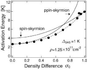
Figure 3: The skyrmion energy is estimated as a function of the imbalanced parameter $\sigma_{0}$ with sample parameters $\Delta_{\text{SAS}}=1$K, and $\rho_{0}=1.2\times 10^{11}$/cm². The experimental data are taken from Terasawa et al.Terasawa04 . Solid lines show the energies of a ppin-skyrmion and a spin-skyrmion, normalized to the data at the balanced point and the monolayer point, respectively. The experimental data would be explained by the excitation of a genuine SU(4) skyrmion.

We proceed to estimate the energies of a spin-skyrmion and a ppin-skyrmion in all range of $\sigma_{0}$, because their estimation is much more reliable than that of a generic SU(4) skyrmion. We use sample parameters $\rho_{0}=1.2\times 10^{11}$/cm², $d=31$Å and $\Delta_{\text{SAS}}=1$K, and normalize the energy to the experimental dataTerasawa04 at the monolayer point for a spin-skyrmion and at the balanced point for a ppin-skyrmion. Recall that the absolute value of the activation energy cannot be determined theoretically because they depends essentially on samples.

First, we calculate the energy of a spin-skyrmion as a function of $\sigma_{0}$ by setting $\kappa=\kappa_{s}$ and $\kappa_{p}=0$ in (156). The skyrmion scale $\kappa$, to be determined by minimizing this, depends on $\sigma_{0}$ very weakly. We obtain $N_{\text{spin}}(\kappa)\simeq 3.5$ as in the monolayer QH ferromagnetEzawa99L ; BookEzawa . We have depicted the excitation energy $E_{\text{sky}}^{\text{spin}}$ in FIG.3, where it is normalized to the data at the monolayer point.

Next, we calculate the energy of a ppin-skyrmion as a function of $\sigma_{0}$ by setting $\kappa=\kappa_{p}$ and $\kappa_{s}=0$ in (156). There is an important remark. The effective tunneling gap diverges as $\sigma_{0}\rightarrow 1$ unless $\Delta_{\text{SAS}}=0$. Furthermore, the minimum pseudospin flip is $N_{\text{ppin}}=1$ for a skyrmion-antiskyrmion pair. Hence, the pair excitation energy (141) diverges as

$$\Delta_{\text{pair}}\rightarrow\frac{\Delta_{\text{SAS}}}{\sqrt{1-\sigma_{0}^{2}}},$$ (158)

and ppin-skyrmions are not excited at the monolayer point ($\sigma_{0}\rightarrow 1$). We have depicted the excitation energy $E_{\text{sky}}^{\text{ppin}}$ in FIG.3, where it is normalized to the data at the monolayer point. In so doing we have used the full expression (231) for the capacitance energy $E_{\text{cap}}$ since other terms are as important as (146) for a ppin-skyrmion of an ordinary size.

IX Activation Energy Anomaly

We have studied how one skyrmion evolves continuously from the balanced point ($\sigma_{0}=0$) to the monolayer point ($\sigma_{0}=1$) by changing its shape. It is important how to distinguish various shapes of skyrmions experimentally. As is well known, as the sample is tilted, the activation energy of a spin-skyrmion increases due to the Zeeman energy. On the contrary, the activation energy of a ppin-skyrmion decreases due to the loss of the exchange energy. Thus, the tilted-field method provides us with a remarkable experimental methodMurphy94L ; SawadaX03PE to reveal the existence of various shapes of a skyrmion in bilayer QH systems.

As the sample is tilted, the parallel magnetic field $B_{\parallel}$ is penetrated between the two layers. We take the symmetric gauge generalized as

$$\mathbf{A}=\left(\frac{1}{2}B_{\perp}y+B_{\|}z,-\frac{1}{2}B_{\perp}x,0\right),$$ (159)

where the two layers are placed at $z=\pm d/2$. In the kinetic Hamiltonian (1) the covariant momentum is now different between the two layers,

$$D_{x}= -i\hbar{\frac{\partial}{\partial x}}+{\frac{\hbar}{2\ell_{B}^{2}}}y+\frac{eB_{\|}d}{2}\tau_{z}^{\text{ppin}},$$

$$D_{y}= -i\hbar{\frac{\partial}{\partial y}}-{\frac{\hbar}{2\ell_{B}^{2}}}x.$$ (160)

Consequently, the LLL condition (130) is modified as

$$(\mathcal{D}_{x}+ i\mathcal{D}_{y})\Phi(\mathbf{x})|\mathfrak{S};B_{\|}\rangle$$

$$= -{\frac{i\hbar}{\ell_{B}}}\left({\frac{\partial}{\partial z^{\ast}}+}\frac{i}{2}\delta_{\text{m}}\ell_{B}\tau_{z}^{\text{ppin}}\right)\Phi(\mathbf{x})|\mathfrak{S};B_{\|}\rangle=0$$ (161)

with

$$\delta_{\text{m}}={\frac{edB_{\|}}{\hbar}}.$$ (162)

We may solve the LLL condition (161) for the one-body wave function $\mathfrak{S}(\mathbf{x};B_{\|})=\langle\mathbf{x}|\mathfrak{S};B_{\|}\rangle$ as

$$\mathfrak{S}(\mathbf{x};B_{\|})=\exp\left({-}\frac{i}{2}\delta_{\text{m}}\tau_{z}^{\text{ppin}}x\right)\mathfrak{S}(z).$$ (163)

Accordingly, the skyrmion configuration acquires different phase factors between the two layers,

$$\mathbf{n}(\mathbf{x};B_{\|})=\exp\left({-}\frac{i}{2}\delta_{\text{m}}\tau_{z}^{\text{ppin}}x\right)\mathbf{n}(\mathbf{x};0),$$ (164)

where $\mathbf{n}(\mathbf{x};0)$ is the configuration (132) in the absence of the parallel magnetic field. Various isospin fields are given by (125) with this CP³ field.

We first consider the balanced configuration ($\sigma_{0}=0$), where we assume ppin-skyrmions are excited [FIG.3]. The excitation energy at $B_{\|}=0$ is given by,

$$E_{\text{sky}}^{\text{ppin}}(0)=E_{\text{X}}^{\text{ppin}}(0)+E_{\text{self}}+E_{\text{cap}}+N_{\text{ppin}}\Delta_{\text{SAS}}{,}$$ (165)

where $E_{\text{X}}^{\text{ppin}}(0)$ is the exchange energy (149) in the absence of the parallel magnetic field. We analyze how the exchange Hamiltonian (121) is affected by the parallel magnetic field. Subtracting the ground-state energy we easily deduce the $B_{\|}$ dependence of the excitation energy,

$$E_{\text{X}}^{\text{ppin}}(B_{\|})=E_{\text{X}}^{\text{ppin}}(0)+\Delta E_{\text{X}}^{\text{ppin}}(B_{\|})$$ (166)

with

$$\Delta E_{\text{X}}^{\text{ppin}}(B_{\|})=-2J_{s}^{d}\delta_{m}^{2}\int\!d^{2}x\,\left(\mathcal{P}_{z}^{\text{sky}}(\mathbf{x})\right)^{2},$$ (167)

where $\mathcal{P}_{z}^{\text{sky}}$ is the skyrmion pseudospin component in the absence of the parallel magnetic field and given by (142).

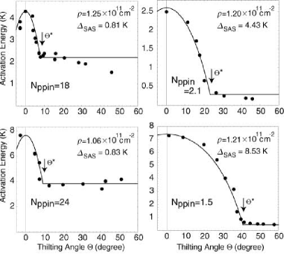
Figure 4: The activation energy at $\nu=1$ is plotted as a function of the tilting angle $\Theta$ in several samples with different tunneling gaps $\Delta_{\text{SAS}}$. It shows a rapid decrease towards the critical angle $\Theta^{\ast}$, and then becomes almost flat. The data are taken from Murphy et al.Murphy94L . They are well fitted by the theoretical formula (169), where the activation energy decreases in the commensurate phase and becomes flat in the incommensurate phase. To fit the data, we have adjusted the activation energy at $\Theta=0$ with the experimental value, and assumed that the number of flipped pseudospins $N_{\text{ppin}}$ is constant for all values of the tilting angle.

We note that $\Delta E_{\text{X}}^{\text{ppin}}(B_{\|})$ is proportional to the capacitance energy (118). Thus the leading order term is found to be

$$\Delta E_{\text{X}}^{\text{ppin}}(B_{\|})\simeq-\frac{2\pi d^{2}J_{s}^{d}}{\ell_{B}^{2}}N_{\text{ppin}}\tan^{2}\Theta,$$ (168)

where $\tan\Theta=B_{\|}/B_{\perp}$ and $N_{\text{ppin}}$ is the number of pseudospins flipped around the skyrmion. All other terms in (165) are unaffected by the parallel magnetic fieldBookEzawa . Thus, the excitation energy decreases as the tilting angle $\Theta$ increases. The rate of the decrease depends on the number $N_{\text{ppin }}$of flipped pseudospins and the amount of the penetrated magnetic field $B_{\|}$.

It has been shownMoon95B ; BookEzawa that, when the parallel magnetic field $B_{\|}$ increases more than a certain critical point, the phase transition occurs in the bilayer QH system: It is the commensurate-incommensurate transition point $B_{\|}^{\ast}$. In the incommensurate phase the penetrated magnetic field is not increased more than $B_{\|}^{\ast}$, because the excess magnetic field $\Delta B_{\|}^{\ast}=B_{\|}^{\ast}-B_{\|}^{\ast}$ is eaten up to create penetrated sine-Gordon vortices between the layers. Hence, the activation energy becomes flat for $\Theta>\Theta^{\ast}$, where $\tan\Theta^{\ast}=B_{\|}^{\ast}/B_{\perp}$.

Hence, from (166) and (168) the excitation energy is

$$E_{\text{sky}}^{\text{ppin}}(B_{\parallel})=E_{\text{X}}^{\text{ppin}}(0)+E_{\text{self}}+E_{\text{cap}}+N_{\text{ppin}}\Delta_{\text{SAS}}^{\Theta}{,}$$ (169)

where we have absorbed $\Delta E_{\text{X}}^{\text{ppin}}(B_{\parallel})$ into the effective tunneling gap,

$$\Delta_{\text{SAS}}^{\Theta}=\left\{\begin{array}[]{ll}\Delta_{\text{SAS}}-(2\pi d^{2}J_{s}^{d}/\ell_{B}^{2})\tan^{2}\Theta&\text{for}\quad\Theta<\Theta^{\ast}\\[8.53581pt] \Delta_{\text{SAS}}-(2\pi d^{2}J_{s}^{d}/\ell_{B}^{2})\tan^{2}\Theta^{\ast}&\text{for}\quad\Theta>\Theta^{\ast}\end{array}\right..$$ (170)

At each angle $\Theta$, in principle, it is necessary to minimize the total excitation energy (169) and determine the scale parameter $\kappa$. However, since the energy change (170) is quite small compared with the total energy, we may treat it as a small perturbation. Namely, we may assume that the flipped pseudospin number $N_{\text{ppin}}$ is a constant independent of $\Theta$. This reminds us of experimental dataMelinte99L ; Kumada00L , where the flipped spin number $N_{\text{spin}}$ is nearly constant by tilting the sample in the excitation of spin-skyrmions.

We have fitted the data due to Murphy et al.Murphy94L in FIG.4 by assuming an appropriate flipped pseudospin number $N_{\text{ppin}}$ per one skyrmion-antiskyrmion pair. We summarize the result in a table.

sample A B C D

$$\Delta_{\text{SAS}}$$

(171)

It takes a large value in samples with $\Delta_{\text{SAS}}<1$ K but take a small value in samples with $\Delta_{\text{SAS}}>4$ K. Recall spin-skyrmion excitations in the monolayer QH system, where the flipped spin number remains small when the Zeeman energy is moderate but becomes quite large when the Zeeman energy is almost zero.

We proceed to analyze excitations of SU(4) skyrmions (164) with (132) in imbalanced configuration, where the exchange Hamiltonian is given by (119). After some calculation we find that the exchange-energy loss $\Delta E_{\text{X}}^{\text{SU(4)}}(B_{\parallel})$ is again proportional to the capacitance energy, and the leading order term is

$$\Delta E_{\text{X}}(B_{\parallel})\simeq-\frac{2\pi d^{2}J_{s}^{d}}{\ell_{B}^{2}}(1-\sigma_{0}^{2})N_{\text{ppin}}\tan^{2}\Theta,$$ (172)

which is reduced to (168) in the balanced point.

Hence, in the commensurate phase ($\Theta<\Theta_{\sigma}^{\ast}$) the excitation energy turns out to be

$$E_{\text{sky}}(B_{\parallel})= E_{\text{X}}(0)+E_{\text{self}}+E_{\text{cap}}{+}N_{\text{spin}}\sqrt{1+\tan^{2}\Theta}\Delta_{\text{Z}}$$

$$+N_{\text{ppin}}\Delta_{\text{BAB}}^{\Theta}$$ (173)

with

$$\Delta_{\text{BAB}}^{\Theta}={\frac{1}{\sqrt{1-\sigma_{0}^{2}}}}\Delta_{\text{SAS}}-\frac{2\pi d^{2}J_{s}^{d}}{\ell_{B}^{2}}(1-\sigma_{0}^{2})\tan^{2}\Theta.$$ (174)

In the incommensurate phase ($\Theta>\Theta_{\sigma}^{\ast}$) it is given by this formula by replacing $\tan^{2}\Theta$ with $\tan^{2}\Theta_{\sigma}^{\ast}$. Here, the commensurate-incommensurate transition point increases slowly asHanna01B

$$\Theta_{\sigma}^{\ast}=(1-\sigma_{0}^{2})^{-1/4}\Theta^{\ast},$$ (175)

as the imbalance parameter $\sigma_{0}$ increases.

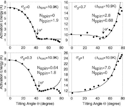
Figure 5: The activation energy at $\nu=1$ is plotted as a function of $\Theta$ in one sample ($\Delta_{\text{SAS}}=11$ K, $\rho_{0}=0.6\times 10^{11}$/cm²) with different imbalance parameter $\sigma_{0}$. It shows a decrease towards the critical angle $\Theta^{\ast}$, and then begin to increase for $\sigma_{0}=0.3$ and $\sigma_{0}=0.7$. The data are taken from Sawada et al.SawadaX03PE . To fit the data by the theoretical formula (173), we have adjusted the activation energy at $\Theta=0$ with the experimental value, and assumed that the flipped spin number $N_{\text{ppin}}$ and the flipped pseudospin number $N_{\text{ppin}}$ are constant for all values of the tilting angle.

Experiments have been carried out by Sawada et al.SawadaX03PE in bilayer samples (FIG.5), where the activation energy was measured at $\nu=1$ by controlling both the tilting angle $\Theta$ and the imbalance parameter $\sigma_{0}$. Their data are interpreted based on the theoretical result (173) as follows. We focus on the behavior of the activation energy $E_{\text{sky}}$ by changing the tilting angle at each fixed imbalance parameter. The relevant term in (173) is

$$\Delta E_{\text{sky}}(\Theta)= N_{\text{spin}}\sqrt{1+\tan^{2}\Theta}\Delta_{\text{Z}}^{0}$$

$$-N_{\text{ppin}}\frac{2\pi d^{2}J_{s}^{d}(1-\sigma_{0}^{2})}{\ell_{B}^{2}}\tan^{2}\Theta$$ (176)

for $\Theta<\Theta_{\sigma}^{\ast}$. By adjusting the theoretical curve to the data at the point $\Theta=0$, we fit the data by this curve throughout the observed range of the tilting angle $\Theta$. As seen in FIG.5, the fitting is quite good when by assuming constant values of $N_{\text{spin}}$ and $N_{\text{ppin}}$ throughout the range of $\Theta$. A deviation of the theoretical curve from the data for large tilting angles $\Theta>70^{\circ}$ would be due to effects not taken into account in the above analysis. For instance, when the parallel magnetic field become too large, the soliton lattice becomes too dense in the incommensurate phase and would destabilize skyrmions. We summarize the numbers $N_{\text{spin}}$ and $N_{\text{ppin}}$ per one skyrmion-antiskyrmion pair determined by this fitting in a table. As the sample is tilted, $N_{\text{spin}}$ increases and $N_{\text{ppin}}$ decreases. In particular, both spins and pseudospins are flipped unless $\sigma_{0}=0$ or $\sigma_{0}=1$. We conclude that the SU(4) skyrmion evolves continuously from the ppin-skyrmion limit to the spin-skyrmion limit as $\sigma_{0}$ increases from $0$ to $1$.

$$\sigma_{0}$$

(177)

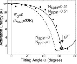
Figure 6: The activation energy at $\nu=1$ is plotted as a function of $\Theta$ in a sample ($\Delta_{\text{SAS}}=33$K, $\rho_{0}=1.0\times 10^{11}$/cm²) . The data are taken from Terasawa et al.Terasawa04 . To fit the data by the theoretical formula, we have adjusted the activation energy at $\Theta=0$ with the experimental value. We have also assumed that $N_{\text{spin}}$ and $N_{\text{ppin}}$ are constant for all values of the tilting angle. A better fitting is obtained as indicated by a solid line when both spins and speudospins are excited.

It is interesting to study the same problem in a sample having a very large tunneling gap. Terasawa et al.Terasawa04 have measured the activation energy by controlling the tilting angle $\Theta$ at the balanced point in a sample with $\Delta_{\text{SAS}}\simeq 33$K. We have fitted their data [FIG.6] by the ppin-excitation formula (169) and by the generic formula (173). It is difficult to fit the data if pure pseudospin excitations are assumed since it is required that $N_{\text{ppin}}\geq 1$ per one pair. A better fitting is obtained if spins and pseudospins are excited simulaneously since $N_{\text{ppin}}$ may take a smaller value than 1. Such a simultaneous excitation is allowed at the balanced point as explained in Appendix D.

In passing we comment on the original mechanismMoon95B ; Yang95B ; Read95B proposed to explain the activation energy anomaly based on the exchange-energy loss of bimeron excitations. A bimeron has the same quantum numbers as a skyrmion, and it can be viewed as a deformed skyrmion with two meron cores with a string between them. The bimeron excitation energy consists of the core energy, the string energy and the Coulomb repulsive energy between the two cores. It is argued that the parallel magnetic field decreases the string tension and hence the bimeron activation energy. Clearly the mechanism works well only when the string length is much larger than the core size. A microscopic calculation has already revealedBrey96B that the meron core size is large enough to invalidate the naive picture. Furthermore, the skyrmion is almost as small as the hole itself in samples with large tunneling gap. On the contrary, in our mechanism the decrease of the exchange energy follows simply from the phase difference induced by the parallel magnetic field between the wave functions associated with the two layers, and it is valid even for small skyrmions.

X Discussion

We have investigated the dynamics of bilayer QH systems based on an algebraic method inherent to the noncommutative plane with $[X,Y]=-i\ell_{B}^{2}$. The noncommutativity induced by the LLL projection implies that the electron position cannot be localized to a point but to a Landau site occupying an area $2\pi\ell_{B}^{2}$. We have derived the Landau-site Hamiltonian $H_{\text{C}}$ akin to the lattice Hamiltonian. It has two entirely different forms, the direct-interaction form $H_{\text{D}}$ and the exchange-interaction form $H_{\text{X}}$. They are equivalent, $H_{\text{D}}=H_{\text{X}}$, as the microscopic Hamiltonian. Nevertheless, the energy of a charge excitation consists of two well-separated pieces, the direct energy $H_{\text{D}}^{\text{cl}}$ and the exchange energy $H_{\text{X}}^{\text{cl}}$.

One of our new contributions is the derivation of various LLL-projected Coulomb potentials in analytic forms. For instance, we have revealed a new form of the capacitance energy (118) with $\epsilon_{\text{cap}}=4(\epsilon_{\text{D}}^{-}-\epsilon_{\text{X}}^{-})$. It is a sum of the direct and exchange Coulomb interaction effects, where the direct effect yields the well-known result from the planar condenser proportional to the layer separation, while the exchange effect gives a quite large negative contribution to it when the layer separation is small enough.

We have explored various aspects of SU(4) skyrmions at $\nu=1$. In particular we have studied a skyrmion-antiskyrmion pair in its small size limit (electron-hole pair) and its large size limit.

The excitation energy of an electron-hole pair is exactly calculable. We have obtained the excitation energy as a function of the imbalance parameter $\sigma_{0}$. The result is quite interesting: At the balanced point ($\sigma_{0}=0$) the pseudospin excitation occurs provided the tunneling gap is not too large ($\Delta_{\text{SAS}}-\Delta_{\text{Z}}<2\epsilon_{\text{X}}^{-}$). A peculiar feature is that, as $\sigma_{0}$ increases, the spin excitation occurs suddenly because the excitation involves just one electron or hole. At the monolayer point ($\sigma_{0}=1$) only spins are excited always. We have also extended the microscopic theory of skyrmionsFertig94B to our framework. However, a quantitative analysis is yet to be carried out.

We then have estimated the SU(4) skyrmion excitation energy as a function of $\sigma_{0}$ based on the effective Hamiltonian valid for very smooth isospin textures. In typical samples it flips only pseudospins at the balanced point. As $\sigma_{0}$ increases, it evolves continuously to flip both spins and pseudospins, and finally flips only spins at the monolayer point. We have then calculated how the excitation energy changes as the sample is tilted. Our formula has explained quite well the activation energy anomaly found by Murphy et al.Murphy94L at the balanced point by excitations of pseudospins, and also found by Sawada et al.SawadaX03PE at various values of $\sigma_{0}$ by simultaneous excitations of spins and pseudospins. Though our formulas are derived for sufficiently smooth skyrmions, they have turned out to be quite good at least with the use of phenomenological values of $N_{\text{spin}}$ and $N_{\text{ppin}}$. We wish to develop a microscopic theory to analyze small skyrmions in a future work. In conclusion, the activation energy anomaly is explained by the loss of the exchange energy of SU(4) skyrmions, which are reduced always to spin-skyrmions at the monolayer point and mostly to pseudospin-skyrmions at the balanced point.

Appendix A Group SU(4)

The special unitary group SU(N) has ($N^{2}-1)$ generators. In the standard representationBookGellMann , we denote them as $\lambda_{A}$, $A=1,2,\cdots,N^{2}-1$, and normalize them as

$$\text{Tr}(\lambda_{A}\lambda_{B})=2\delta_{AB}.$$ (178)

They are characterized by

$$[\lambda_{A},\lambda_{B}]= 2if_{ABC}\lambda_{C},$$

$$\{\lambda_{A},\lambda_{B}\}= \frac{4}{N}+\delta_{AB}2d_{ABC}\lambda_{C},$$ (179)

where $f_{ABC}$ and $d_{ABC}$ are the structure constants of SU(N). We have $\lambda_{A}=\tau_{A}$ (the Pauli matrix) with $f_{ABC}=\varepsilon_{ABC}$ and $d_{ABC}=0$ in the case of SU(2).

This standard representation is not convenient for our purpose because the spin group is SU(2)$\otimes$SU(2) in the bilayer electron system with the four-component electron field as $\Psi=(\psi^{\text{f}\uparrow},\psi^{\text{f}\downarrow},\psi^{\text{b}\uparrow},\psi^{\text{b}\downarrow})$. Embedding SU(2)$\otimes$SU(2) into SU(4) we define the spin matrix by

$$\tau_{x}^{\text{spin}}= \left(\begin{array}[]{cc}\tau_{x}&0\\ 0&\tau_{x}\end{array}\right),\quad\tau_{y}^{\text{spin}}=\left(\begin{array}[]{cc}\tau_{y}&0\\ 0&\tau_{y}\end{array}\right),$$ (184)

$$\tau_{z}^{\text{spin}}= \left(\begin{array}[]{cc}\tau_{z}&0\\ 0&\tau_{z}\end{array}\right),$$ (187)

and similarly the pseudospin matrix by

$$\tau_{x}^{\text{ppin}}= \left(\begin{array}[]{cc}0&\mathbf{1}_{2}\\ \mathbf{1}_{2}&0\end{array}\right),\quad\tau_{y}^{\text{ppin}}=\left(\begin{array}[]{cc}0&-i\mathbf{1}_{2}\\ i\mathbf{1}_{2}&0\end{array}\right),$$ (192)

$$\tau_{z}^{\text{ppin}}= \left(\begin{array}[]{cc}\mathbf{1}_{2}&0\\ 0&-\mathbf{1}_{2}\end{array}\right),$$ (195)

where $\mathbf{1}_{2}$ is the unit matrix in two dimensions. Nine remaining matrices are products of the spin and pseudospin matrices:

$$\tau_{a}^{\text{spin}}\tau_{x}^{\text{ppin}}= \left(\begin{array}[]{cc}0&\tau_{a}\\ \tau_{a}&0\end{array}\right),\quad\tau_{a}^{\text{spin}}\tau_{y}^{\text{ppin}}=\left(\begin{array}[]{cc}0&-i\tau_{a}\\ i\tau_{a}&0\end{array}\right),$$ (200)

$$\tau_{a}^{\text{spin}}\tau_{z}^{\text{ppin}}= \left(\begin{array}[]{cc}\tau_{a}&0\\ 0&-\tau_{a}\end{array}\right).$$ (203)

Let us denote them as $T_{A}$, $A=1,2,\cdots,15$, where $T_{1}=T_{x0}$, etc., $T_{4}=T_{0x}$, etc., $T_{7}=T_{xx}$, $T_{8}=T_{xy}$, etc. with $T_{a0}\equiv\tau_{a}^{\text{spin}},\quad T_{0a}\equiv\tau_{a}^{\text{ppin}},\quad T_{ab}\equiv\tau_{a}^{\text{spin}}\tau_{b}^{\text{ppin}}$. They are related with the standard SU(4) generators as

$$T_{x0} =\lambda_{1}+\lambda_{13},\quad T_{y0}=\lambda_{2}+\lambda_{14},$$

$$T_{z0} =\lambda_{3}-\frac{1}{\sqrt{3}}\lambda_{8}+\frac{\sqrt{6}}{3}\lambda_{15},$$

$$T_{0x} =\lambda_{4}+\lambda_{11},\quad T_{0y}=\lambda_{5}+\lambda_{12},$$

$$T_{0z} =\frac{2}{\sqrt{3}}\lambda_{8}+\frac{2}{\sqrt{6}}\lambda_{15},$$

$$T_{xx} =\lambda_{6}+\lambda_{9},\quad T_{xy}=\lambda_{10}+\lambda_{7},\quad T_{xz}=\lambda_{1}-\lambda_{13},$$

$$T_{yx} =\lambda_{10}-\lambda_{7},\quad T_{yy}=\lambda_{6}-\lambda_{9},\quad T_{yz}=\lambda_{2}-\lambda_{14},$$

$$T_{zx} =\lambda_{4}-\lambda_{11},\quad T_{zy}=\lambda_{5}-\lambda_{12},$$

$$T_{zz} =\lambda_{3}+\frac{1}{\sqrt{3}}\lambda_{8}-\frac{\sqrt{6}}{3}\lambda_{15}.$$ (204)

The normalization condition reads

$$\text{Tr}(T_{ab}T_{cd})=4\delta_{ac}\delta_{bd},$$ (205)

which is different from the standard one (178).

Appendix B Decomposition Formula

The Landau-site Hamiltonian $H_{\text{C}}$ possesses two entirely different forms, the direct-interaction form $H_{\text{D}}$ and the exchange-interaction form $H_{\text{X}}$. They are equivalent, $H_{\text{D}}=H_{\text{X}}$, as the microscopic Hamiltonian. On the other hand, the excitation energy consists of two well-separated pieces, the direct energy and the exchange energy. In this appendix we derive the decomposition formula (40),

$$\langle\mathfrak{S}|H_{\text{C}}|\mathfrak{S}\rangle=H_{\text{D}}^{\text{cl}}+H_{\text{X}}^{\text{cl}},$$ (206)

for skyrmion excitations. We also prove the algebraic relation (27), or

$$\sum_{A=1}^{N^{2}-1}\widehat{I}_{A}^{\text{cl}}(\mathbf{x})\bigstar\widehat{I}_{A}^{\text{cl}}(\mathbf{x})+\frac{1}{2N}\widehat{\rho}^{\text{cl}}(\mathbf{x})\bigstar\widehat{\rho}^{\text{cl}}(\mathbf{x})=\frac{1}{4\pi\ell_{B}^{2}}\widehat{\rho}^{\text{cl}}(\mathbf{x}),$$ (207)

that holds among the classical densities associated with the generators of the W_∞(N) algebra.

We consider a skyrmion state in the SU(N) QH ferromagnet,

$$|\mathfrak{S}\rangle=\prod_{n=0}\xi^{\dagger}(n)|0\rangle,$$ (208)

where

$$\xi^{\dagger}(n)=\sum_{\mu}^{N}\left[u_{\mu}(n)c_{\mu}^{\dagger}(n)+v_{\mu}(n)c_{\mu}^{\dagger}(n+1)\right].$$ (209)

They satisfy the standard canonical commutation relations,

$$[\xi(m),\xi^{\dagger}(n)]=\delta_{mn},\quad[\xi(m),\xi(n)]=0,$$ (210)

provided

$$\sum_{\mu}^{N}\left[u_{\mu}(n)u_{\mu}^{\dagger}(n)+v_{\mu}(n)v_{\mu}^{\dagger}(n)\right]= 1,$$

$$\sum_{\mu}^{N}v_{\mu}^{\dagger}(n)u_{\mu}(n+1)= 0.$$ (211)

It follows that

$$c_{\mu}(n)|\mathfrak{S}\rangle=\left[u_{\mu}(n)\xi(n)+v_{\mu}(n-1)\xi(n-1)\right]|\mathfrak{S}\rangle,$$ (212)

from which the only nonvanishing components of two-point correlation functions are found to be

$$\langle c_{\mu}^{\ast}(n)c_{\nu}(n)\rangle=u_{\mu}^{\ast}(n)u_{\nu}(n)+v_{\mu}^{\ast}(n-1)v_{\nu}(n-1),$$

$$\langle c_{\mu}^{\ast}(n)c_{\nu}(n+1)\rangle=u_{\mu}^{\ast}(n)v_{\nu}(n),$$ (213)

where $\langle c_{\mu}^{\ast}(n)c_{\nu}(n)\rangle=\langle\mathfrak{S}|c_{\mu}^{\ast}(n)c_{\nu}(n)|\mathfrak{S}\rangle$ and so on. We also derive

$$c_{\mu}(j)c_{\nu}(n)|\mathfrak{S}\rangle= \left[u_{\mu}(j)\xi(j)+v_{\mu}(j-1)\xi(j-1)\right]$$

$$\times\left[u_{\nu}(n)\xi(n)+v_{\nu}(n-1)\xi(n-1)\right]|\mathfrak{S}\rangle.$$ (214)

Four-point correlation functions $\langle c_{\mu}^{{\dagger}}(m)c_{\sigma}^{{\dagger}}(i)c_{\tau}(j)c_{\nu}(n)\rangle$ are complicated. Nevertheless, taking into account the angular-momentum conservation ($V_{mnij}\varpropto\delta_{m+i,n+j}$) we deduce

$$V_{mnij} \left\langle c_{\mu}^{{\dagger}}(m)c_{\sigma}^{{\dagger}}(i)c_{\tau}(j)c_{\nu}(n)\right\rangle$$

$$= V_{mnij}\left\langle c_{\mu}^{{\dagger}}(m)c_{\nu}(n)\right\rangle\left\langle c_{\sigma}^{{\dagger}}(i)c_{\tau}(j)\right\rangle$$

$$-V_{mnij}\left\langle c_{\mu}^{{\dagger}}(m)c_{\tau}(j)\right\rangle\left\langle c_{\sigma}^{{\dagger}}(i)c_{\nu}(n)\right\rangle.$$ (215)

This is the general expression allowing to express all kind of Coulomb energies in the exact form.

It follows from (215) that

$$V_{mnij}\sum_{\mu\nu\tau\nu}\left\langle c_{\mu}^{{\dagger}}(m)c_{\sigma}^{{\dagger}}(i)c_{\tau}(j)c_{\nu}(n)\right\rangle\delta_{\mu\nu}\delta_{\sigma\tau}$$

$$= V_{mnij}\rho^{\text{cl}}(m,n)\rho^{\text{cl}}(i,j)-V_{mnij}X(m,n,i,j),$$ (216)

where we have set

$$X(m,n,i,j)\equiv\sum_{\mu\nu\tau\nu}\left\langle c_{\mu}^{{\dagger}}(m)c_{\tau}(j)\right\rangle\left\langle c_{\sigma}^{{\dagger}}(i)c_{\nu}(n)\right\rangle\delta_{\mu\nu}\delta_{\sigma\tau}.$$ (217)

Here we use the algebraic identity (29) to find

$$X(m,n,i,j)=2\left[I_{A}^{\text{cl}}(m,j)I_{A}^{\text{cl}}(i,n)+\frac{1}{2N}\rho^{\text{cl}}(m,j)\rho^{\text{cl}}(i,n)\right].$$ (218)

Consequently,

$$E_{\text{C}}= -\sum_{mnij}{V}_{mnij}\sum_{\sigma,\tau}\langle c_{\sigma}^{\dagger}(m)c_{\tau}^{\dagger}(i)c_{\sigma}(n)c_{\tau}(j)\rangle$$

$$= E_{\text{D}}+E_{\text{X}},$$ (219)

where

$$E_{\text{D}}= \sum_{mnij}{V}_{mnij}\rho^{\text{cl}}(m,n)\rho^{\text{cl}}(i,j),$$ (220)

$$E_{\text{X}}= -2\sum_{mnij}{V}_{mnij}\big{[}\sum_{A=1}I_{A}^{\text{cl}}(m,j)I_{A}^{\text{cl}}(i,n)$$

$$\hskip 57.81621pt+\frac{1}{2N}\rho^{\text{cl}}(m,j)\rho^{\text{cl}}(i,n)\big{]}.$$ (221)

Now, $E_{\text{D}}$ and $E_{\text{X}}$ are identical to (18) and (30) when we replace $\rho(m,n)$ and $I_{A}(m,n)$ with $\rho^{\text{cl}}(m,n)$ and $I_{A}^{\text{cl}}(m,j)$. Hence, we have established the decomposition formula (206) rigorously.

We proceed to prove the algebraic relation (207) for the skyrmion state (208). From (217) we define

$$X(m,n)\equiv\sum_{ij}X(m,n,i,j)\delta_{ij}$$

$$=\sum_{j}\sum_{\mu\sigma}\left\langle c_{\mu}^{{\dagger}}(m)c_{\sigma}(j)\right\rangle\left\langle c_{\sigma}^{{\dagger}}(j)c_{\mu}(n)\right\rangle.$$ (222)

Using (211) and (213) we find the only nonvanishing values to be given by

$$X(n,n)= u^{{\dagger}}(n)u(n)+v^{{\dagger}}(n-1)v(n-1),$$

$$X(n,n+1)= [X(n+1,n)]^{\ast}=u^{{\dagger}}(n)v(n),$$ (223)

which implies that $X(m,n)=\rho^{\text{cl}}(m,n)$. Combining this with (218) we obtain

$$I_{A}^{\text{cl}}(m,l)I_{A}^{\text{cl}}(l,n)+\frac{1}{2N}\rho^{\text{cl}}(m,l)\rho^{\text{cl}}(l,n)=\frac{1}{2}\rho^{\text{cl}}(m,n).$$ (224)

This is equivalent to (207) in the coordinate space.

Appendix C Coulomb Energies

We estimate the Coulomb self-energy of one skyrmion in the bilayer QH ferromagnet. It is defined by

$$E_{\text{self}}=\pi\int\!d^{2}q\,\delta\rho_{\text{sky}}(-\mathbf{q})V^{+}(\mathbf{q})\delta\rho_{\text{sky}}(\mathbf{q})$$ (225)

with

$$V^{+}(q)={\frac{e^{2}}{8\pi\varepsilon q}}\left(1+e^{-qd}\right).$$ (226)

The density modulation $\delta\rho_{\text{sky}}(\mathbf{x})$ is given by (137) for a large skyrmion. Its Fourier component reads

$$\delta\rho_{\text{sky}}(\mathbf{q})=\frac{1}{2\pi}\int\!d^{2}x\,e^{i\mathbf{qx}}\delta\rho_{\text{sky}}(\mathbf{x})=\frac{\alpha q}{2\pi}K_{1}(\alpha q),$$ (227)

where we have set $\alpha=2\kappa\ell_{B}$. To calculate the energy we use (95) and

$$\int\limits_{0}^{\infty}\!dr\,\frac{r^{n+1}\hskip 0.7113ptJ_{n}(qr)}{(r^{2}+\alpha^{2})^{m+1}}=\frac{q^{m}\alpha^{n-m}}{2^{m}m!}K_{n-m}(\alpha q),$$ (228)

where $K_{n}(z)=K_{-n}(z)$ is the modified Bessel function: See the formula (11.4.44) in Ref.Abramowitz . Now it is straightforward to derive

$$E_{\text{self}}=\frac{E_{\text{C}}^{0}}{8\kappa}\int z^{2}[K_{1}(z)]^{2}\left(1+e^{-\frac{d}{2\ell}\frac{z}{\kappa}}\right)dz$$ (229)

as the Coulomb self-energy of one skyrmion.

The SU(4)-noninvariant term yields the capacitance energy (145),

$$E_{\text{cap}}={2}\pi\ell_{B}^{2}\epsilon_{\text{cap}}\int\!d^{2}x\,\delta P_{z}^{\text{sky}}(\mathbf{x})\delta P_{z}^{\text{sky}}(\mathbf{x}),$$ (230)

where $\delta P_{z}^{\text{sky}}(\mathbf{x})$ is given by (139). After some calculation we obtain

$$\frac{E_{\text{cap}}}{\epsilon_{\text{cap}}}= \frac{\sigma_{0}^{2}}{24\kappa^{2}}+(1-\sigma_{0}^{2})\kappa_{p}^{2}A(\kappa)+\sigma_{0}^{2}\left(\frac{1}{4\kappa^{2}}-1\right)\frac{\kappa_{p}^{2}}{2\kappa^{2}}$$

$$+\sigma_{0}^{2}\left(\frac{1}{10\kappa^{2}}-\frac{2}{3}+2\kappa^{2}\right)\frac{\kappa_{p}^{4}}{\kappa^{4}},$$ (231)

where $\alpha=2\kappa\ell_{B}$ and $\alpha_{p}=2\kappa_{p}\ell_{B}$: $A(\kappa)$ is divergent logarithmically,

$$A(\kappa)=\frac{1}{\kappa^{2}}\int_{0}^{\infty}\left(\frac{1}{r^{2}+\alpha^{2}}-\frac{2\alpha^{2}\ell_{B}^{2}}{\left(r^{2}+\alpha^{2}\right)^{3}}\right)^{2}r^{3}dr.$$ (232)

We take the divergent term as the leading contribution for the pseudospin component,

$$E_{\text{cap}}\simeq\frac{1}{2}(1-\sigma_{0}^{2})\epsilon_{\text{cap}}N_{\text{ppin}}(\kappa_{p})$$ (233)

with (155).

Finally we present the formula for the exchange energy (119) for a general SU(4) skyrmion (132). After a straightforward but tedious calculation we obtain

$$E_{\text{X}}^{\text{SU(4)}}$$

$$= 4\pi J_{s}^{+}\left(1+\frac{1}{10\kappa^{4}}\right)-4\pi J_{s}^{-}\left(\frac{1}{3}+\frac{1-3\sigma_{0}^{2}}{140\kappa^{4}}\right)$$

$$+4\pi J_{s}^{-}\left(\frac{2}{3}+\frac{3}{14\kappa^{4}}\right)\left(\sigma_{0}\frac{\kappa_{s}}{\kappa}+\sqrt{1-\sigma_{0}^{2}}\frac{\kappa_{r}}{\kappa}\right)^{2}\frac{\kappa_{s}^{2}}{\kappa^{2}}$$

$$+4\pi J_{s}^{-}\left(\frac{1+\sigma_{0}^{2}}{3}+\frac{1-19\sigma_{0}^{2}}{140\kappa^{4}}\right)\frac{\kappa_{s}^{2}}{\kappa^{2}}$$

$$+4\pi J_{s}^{-}(1-\sigma_{0}^{2})\left(\frac{1}{3}+\frac{1}{140\kappa^{4}}\right)\frac{\kappa_{r}^{2}}{\kappa^{2}}$$

$$+4\pi J_{s}^{-}\sigma_{0}\sqrt{1-\sigma_{0}^{2}}\left(\frac{2}{3}+\frac{9}{70\kappa^{4}}\right)\frac{\kappa_{s}\kappa_{r}}{\kappa^{2}}.$$ (234)

By setting $\kappa_{r}=0$, this is reduced to $E_{\text{X}}^{\text{SU(4)}}=E_{\text{X}}+\Delta E_{\text{X}}$ with (147), where

$$\Delta E_{\text{X}}= \frac{4\pi}{10\kappa^{4}}J_{s}^{+}-\frac{4\pi\kappa_{p}^{2}}{140\kappa^{6}}J_{s}^{-}$$

$$+\frac{4\pi\sigma_{0}^{2}}{140\kappa^{8}}\left[3\kappa^{4}-19\kappa^{2}\kappa_{s}^{2}+30\kappa_{s}^{4}\right]J_{s}^{-}.$$ (235)

The correction term is small for a large skyrmion.

Appendix D Continuous Transformation

Based on the skyrmion-energy formula (156) we verify that, if a ppin-skyrmion ($\kappa_{s}=0$, $\kappa_{p}=\kappa)$ is excited at the balanced point, it evolves continuously into a spin-skyrmion ($\kappa_{s}=\kappa$, $\kappa_{p}=0)$ via a generic skyrmion ($\kappa_{s}\kappa_{p}\neq 0)$ as the imbalance parameter $\sigma_{0}$ increases.

We summarize the total skyrmion energy (156) as a function of $\kappa=\sqrt{\kappa_{s}^{2}+\kappa_{p}^{2}}$, $z=\left(\kappa_{s}/\kappa\right)^{2}$ and $\sigma_{0}$ in the following form,

$$E_{\text{sky}}(\kappa,z;\sigma_{0})=\frac{4\pi J_{s}^{+}\sigma_{0}^{2}}{3}z^{2}+A(\kappa;\sigma_{0})z+B(\kappa;\sigma_{0}),$$ (236)

where

$$A(\kappa;\sigma_{0})= \frac{4\pi J_{s}^{-}}{3}(1+\sigma_{0}^{2})-\frac{1-\sigma_{0}^{2}}{2}\epsilon_{\text{cap}}\kappa^{2}N_{\xi}$$

$$+\Delta_{\text{Z}}\kappa^{2}N_{\xi}-\frac{\Delta_{\text{SAS}}}{\sqrt{1-\sigma_{0}^{2}}}\kappa^{2}N_{\xi}$$ (237)

with (152). The explicit expression of $B(\kappa;\sigma_{0})$ is not necessary. The variable $z$ is limited in the range $0\leq z\leq 1$.

We start with the balanced point ($\sigma_{0}=0$), where $E_{\text{sky}}(\kappa,z;\sigma_{0})$ is a linear function of $z$. Let us assume

$$A(\kappa;\sigma_{0})>0\qquad\text{at\quad}\sigma_{0}=0.$$ (238)

Then the energy is minimized at $z=0$ or $\kappa_{s}=0$, where ppin-skyrmions are excited. We now increases $\sigma_{0}$ from $\sigma_{0}=0$. As far as $A(\kappa;\sigma_{0})>0$, ppin-skyrmions have the lowest energy. Due to the $\Delta_{\text{SAS}}$ term, $A(\kappa;\sigma_{0})$ decreases and vanishes at $\sigma_{0}=\sigma_{\text{p}}$,

$$A(\kappa;\sigma_{0})=0\qquad\text{at\quad}\sigma_{0}=\sigma_{\text{p}}.$$ (239)

Then it becomes negative for $\sigma_{0}>\sigma_{\text{p}}$, and the energy is minimized at $z=z_{\text{min}}$ with

$$z_{\text{min}}=\frac{3}{8\pi J_{s}^{+}\sigma_{0}^{2}}|A(\kappa;\sigma_{0})|.$$ (240)

Because $z_{\text{min}}$ increases continuously from $z_{\text{min}}=0$ at $\sigma_{0}=\sigma_{\text{p}}$, the spin component ($\kappa_{s}$) is excited gradually to form a generic skyrmion ($\kappa_{s}\kappa_{p}\neq 0)$. The point $z_{\text{min}}$ increases and achieve at $z_{\text{min}}=1$ at $\sigma_{0}=\sigma_{\text{s}}$,

$$|A(\kappa;\sigma_{0})|=\frac{8\pi J_{s}^{+}\sigma_{0}^{2}}{3}\qquad\text{at\quad}\sigma_{0}=\sigma_{\text{s}},$$ (241)

where the pseudospin component ($\kappa_{p}$) vanishes continuously.

We conclude that, if $A(\kappa;\sigma_{0})>0$ at $\sigma_{0}=0$, ppin-skyrmions are excited for $0\leq\sigma_{0}<\sigma_{\text{p}}$, generic skyrmions are excited for $\sigma_{\text{p}}<\sigma_{0}<\sigma_{\text{s}}$, and finally spin-skyrmions are excited for $\sigma_{\text{s}}<\sigma_{0}\leq 1$. The transition occurs continuously as illustrated in FIG.3, with the critical points $\sigma_{\text{p}}$ and $\sigma_{\text{s}}$ being fixed by (238) and (241). On the other hand, generic skyrmions are excited at the balanced point if $A(\kappa;\sigma_{0})<0$ and $z_{\text{min}}<1$ at $\sigma_{0}=0$, and spin skyrmions are excited at the balanced point if $A(\kappa;\sigma_{0})<0$ and $z_{\text{min}}\geq 1$ at $\sigma_{0}=0$.

References

(1) Z.F. Ezawa, Quantum Hall Effects: Field
Theoretical Approach and Related Topics (World Scientific, 2000).
(2) S. Das Sarma and A. Pinczuk (eds), Perspectives in Quantum Hall Effects (Wiley, 1997).
(3) I.B. Spielman, J.P. Eisenstein, L.N. Pfeiffer and K.W.
West, Phys. Rev. Lett. 84 (2000) 5808.
(4) Z.F. Ezawa and A. Iwazaki, Int. J. Mod. Phys. B
6 (1992) 3205; Phys. Rev. B 47 (1993) 7295; 48
(1993) 15189.
(5) Z.F. Ezawa, Phys. Rev. B 55 (1997) 7771.
(6) K. Moon, H. Mori, K. Yang, S.M. Girvin, A.H. MacDonald, L.
Zheng, D. Yoshioka and S-C. Zhang, Phys. Rev. B 51 (1995) 5138.
(7) S.L. Sondhi, A. Karlhede, S.A. Kivelson and E.H. Rezayi,
Phys. Rev. B 47 (1993) 16419.
(8) S.E. Barrett, G. Dabbagh, L.N. Pfeiffer, K.W. West and
R. Tycko, Phys. Rev. Lett. 74 (1995) 5112.
(9) E.H. Aifer, B.B. Goldberg and D.A. Broido, Phys. Rev.
Lett. 76 (1996) 680.
(10) A. Schmeller, J.P. Eisenstein, L.N. Pfeiffer and K.W.
West, Phys. Rev. Lett. 75 (1995) 4290.
(11) S.Q. Murphy, J.P. Eisenstein, G.S. Boebinger, L.N.
Pfeiffer and K.W. West, Phys. Rev. Lett. 72 (1994) 728.
(12) Z.F. Ezawa, Phys. Rev. Lett. 82 (1999) 3512.
(13) A. Sawada, Z.F. Ezawa, H. Ohno, Y. Horikoshi, O.
Sugie, S. Kishimoto, F. Matsukura, Y. Ohno and M. Yasumoto, Solid State
Comm. 103 (1997) 447.
(14) A. Sawada, D. Terasawa, N. Kumada, M. Morino, K.
Tagashira, Z.F. Ezawa, K. Muraki, T. Saku and Y. Hirayama, Physica E 18
(2003) 118.
(15) D. Terasawa, M. Morino, K. Nakada, S. Kozumi, A.
Sawada, Z.F. Ezawa, N. Kumada, K. Muraki, T. Saku and Y. Hirayama, Physica E
22 (2002) 52.
(16) Z.F. Ezawa, G. Tsitsishvili and K. Hasebe, Phys. Rev. B
67 (2003) 125314.
(17) H.A. Fertig, L. Brey, R. Cote and A.H. MacDonald, Phys.
Rev. B 50 (1994) 11018.
(18) S. Iso, D. Karabali, and B. Sakita, Phys. Lett. B 196, 143 (1992).
(19) A. Cappelli, C. Trugenberger, and G. Zemba, Nucl.
Phys. B 396 (1993) 465.
(20) S.M.Girvin and T.Jach, Phys. Rev. B 29 (1984)
5617.
(21) S.M.Girvin, A.H.MacDonald and P.M.Platzman, Phys. Rev. B
33 (1986) 2481.
(22) C. Kallin and B.I. Halperin, Phys. Rev. B 30 (1991) 5655.
(23) A.P. Prudnikov, Yu.A. Brychkov and O.I. Marichev,
Integrals and Series, vol.2: Special Functions (Gordon and Breach,
1988)
(24) M. Abramowitz and I.A. Stegun, Handbook of
Mathematical Functions (Dover Publications, New York 1972).
(25) It is found that K
and K while K and K for the
layer separation Å and Å, respectively. (We have taken /cm2.) In our analysis the capacitance
energy is given by (118), where K and K for Å and Å, respectively. In some literatureMoon95B ; Demler99L it is assumed that . The capacitance energy becomes quite small for a small layer
separation due to the exchange interaction.
(26) E. Demler and S. Das Sarma, Phys. Rev. Lett. 82 (1999)
3895.
(27) S.M. Girvin and A.H. MacDonald, Phys. Rev. Lett. 58 (1987) 1252.
(28) N. Read, Phys. Rev. Lett. 62 (1989) 86.
(29) A. D’Adda, A. Luscher and P. DiVecchia, Nucl. Phys. B
146 (1978) 63.
(30) R.B. Laughlin, Phys. Rev. Lett. 50 (1983)
1395.
(31) In computing the activation energy of a skyrmion
or an antiskyrmion, one needs to know the chemical potential to remove or
add an electron to the systemMoon95B . However, this problem does not
exist as far as we consider a skyrmion-antiskyrmion pair because the number
of electrons is unchanged. Thus, when we calculate the skyrmion energy, we
actually consider the energy of a skyrmion in a well-separated
skyrmion-antiskyrmion pair.
(32) N. Kumada, A. Sawada, Z.F. Ezawa, S. Nagahama, H.
Azuhata, K. Muraki, T. Saku and Y. Hirayama, J. Phys. Soc. Jap. 69 (2000)
3178.
(33) S. Melinte, E. Grivei, V. Bayot and M. Shayegan, Phys.
Rev. Lett. 82 (1999) 2764.
(34) C.B. Hanna and A.H. MacDonald and S.M. Girvin, Phys.
Rev. B 63 (2001) 125305.
(35) K. Yang and A.H. MacDonald, Phys. Rev. B 51 (1995) 17247.
(36) N. Read, Phys. Rev. B 52 (1995) 1926.
(37) L. Brey, H.A. Fertig, R. Cote and A.H. MacDonald, Phys.
Rev. B 54 (1996) 16888.
(38) M.Gell-Mann and Y. Ne’eman, The eight-fold Way
(Benjamin, New York, 1964).