Exact ground-state for the periodic Anderson model in $D=2$ dimensions at finite value of the interaction and absence of the direct hopping in the correlated f-band.

Abstract

We report for the first time exact ground-states deduced for the $D=2$ dimensional generic periodic Anderson model at finite $U$, the Hamiltonian of the model not containing direct hopping terms for $f$-electrons $(t^{f}=0)$. The deduced itinerant phase presents non-Fermi liquid properties in the normal phase, emerges for real hybridization matrix elements, and not requires anisotropic unit cell. In order to deduce these results, the plaquette operator procedure has been generalised to a block operator technique which uses blocks higher than an unit cell and contains $f$-operator contributions acting only on a single central site of the block.

I Introduction

The periodic Anderson model (PAM) is one of the basic models largely used in the study of strongly correlated systems whose properties can be described at the level of two effective bands, like heavy-fermion systems [1], intermediate-valence compounds [2], or even high critical temperature superconductors [3]. The model contains a free $d$ band hybridized with a correlated system of $f$ electrons for which the one-site Coulomb repulsion in the form of the Hubbard interaction is locally present. Seen from the theoretical side, PAM has the peculiarity that even its one dimensional Hamiltonian is sufficiently complicated to not allow the knowledge of its exact solutions even in 1D. As a consequence, taking into account that the exact description possibilities increase in difficulty with the increase of the dimensionality of the system in the physical region $D=1-3$, the physics provided by PAM is almost exclusively interpreted based on approximations. This situation enhance the difficulty of a good quality theoretical analysis, since exact bench-marks in testing the approximations or numerical simulations are almost completely missing. Because of this fact, even the starting point of the theoretical description, the knowledge of the ground-state is poorly developing. Given by this, efforts have been made for the construction of exact ground-states at least in restricted regions of the parameter space. In this frame, based on the observation that the infinitely repulsive case in relative terms is easier to treat, the first exact ground-states have been deduced at $U=\infty$, in restricted regions of the parameter space, based on a work of several years [4, 5, 6, 7].

The first exact ground-states at finite value of the interaction have been published recently in 1D [8, 9], and 2D [10, 11], respectively. These ground-states emerge on continuous but restricted regions of the $T=0$ phase diagram of the system which extend from the low $U$ limit up to the high $U$ limit as well. These solutions have been obtained by a decomposition of the Hamiltonian in positive semidefinite operators (PSO) as follows (i) the interaction term has been transformed into a PSO requiring at least one $f$ electron on every lattice site [8], and (ii) the remaining parts of the interaction term together with the one-particle components of the Hamiltonian have been transformed in PSO based on cell operators, using bonds in 1D [8, 9] or elementary plaquette operators in 2D [10, 11, 12]. Two type of ground-states have been obtained in this manner: localized and itinerant once. The itinerant solution was found to emerge for imaginary hybridization matrix elements ($V_{\bf r}$), while the localized solution for real $V_{\bf r}$. Besides, the itinerant solution has been obtained only in the presence of anisotropic or distorted unit cells. The cell operators used in the transformation of the Hamiltonian had always the extension of an unit cell (elementary plaquette in 2D), the $f$-creation operators being ,,uniformly” considered, acting on all lattice sites of the elementary plaquette.

We must note, that all exact ground-states deduced up today for PAM at finite value of the interaction $U$, based on the cell operators mentioned above, require the presence of the direct hopping $t^{f}\neq 0$ as well in the correlated $f$ band of the Hamiltonian, since the products of these cell operators leading to PSO generate always $t^{f}\neq 0$ contributions. The presence of the direct $f$ hopping can be argued based on experimental data in the case of $Pu$ [13], or some heavy-fermion compounds [14], but it remains in fact an extension term to the generic PAM Hamiltonian which does not contain such type of contributions. Particularly for 2D, since for the $t^{f}=0$ limit the results deduced in Refs.[[10, 11]] are no more valid, the case of the generic PAM Hamiltonian treated in exact terms remains still a completely open problem.

Driven by the challenge to obtain exact solutions for the generic PAM in 2D, the first questions which have to be clarified in these conditions are the following: Can we consider the ground-states deduced for PAM at finite $U$ in the presence of direct $f$ hopping in the Hamiltonian also potential ground-states for the generic PAM at finite $U$ (and $t^{f}=0$) ? The unit cell distortions and imaginary hybridization matrix elements are essential for the emergence of itinerant phases ? This questions are important, since are connected to main problems related to PAM, for example the localized vs. itinerant behaviour of $f$-electrons, and of particles in general in the system [15, 16, 17, 18, 19, 20], or the interpretation of the PAM behaviour based exclusively on the local $f$-moment and its compensation (analyses made based on Kondo physics).

Starting from this background, in this paper we are reporting the first exact ground-states for generic PAM in 2D at finite value of the interaction. As a consequence, the deduction is made without the presence of the direct hopping terms for $f$ electrons in the Hamiltonian of the model ($t^{f}=0)$. The obtained exact ground-state is itinerant, emerges for real values of the Hamiltonian parameters (including the hybridization matrix elements as well), is not necessarily connected to distorted unit cells and presents clear similarities in its physical properties with the itinerant solution obtained in the presence of direct $f$ hopping terms in $\hat{H}$ [10]. Since the momentum distribution function is continuous without any non-regularities in its derivatives of any order, the presented ground-state is a non-Fermi liquid state in the normal phase, possesses a large spin degeneracy, and globally is paramagnetic.

In order to deduce the reported results, major developments have been applied in comparison with the plaquette operator method used in Ref.([10]) and described in detail in Ref.([11]), which has been generalised to a block operator procedure. The introduced block is qualitatively different from the elementary plaquette previously used since a) it has an extension greater than an unit cell and b) it contains $f$ creation operators acting only on one unique central site of the block. This choice allows us to represent the PAM Hamiltonian in term of PSO block products even in the absence of the direct $f$ hopping terms and to obtain non-localized ground-states in the presence of real hybridization matrix elements and absence of lattice distortions. All these are not possible to obtain in the frame of Refs.[[10, 11]].

The consequences of the presented results are multiple. (i) At the level of exact solutions in 2D, the difference between the case $t^{f}\neq 0$ and $t^{f}=0$ in $\hat{H}$, (at least at the level of known exact ground-states) seems to not be extremely significant. Physically this can be understood based on the hybridization term which allows the movement of $f$-electrons even if direct hopping in the correlated band is not present in $\hat{H}$, and, in fact for the behaviour of the system (and also the ground-state), not the bare bands are important but the diagonalized once. For the presented case the $t^{f}\neq 0$ value seems only to shift the position in the parameter space of the emerging phase in comparison with the $t^{f}=0$ situation, without changing essentially its physical properties. (ii) The fact that similar phases are obtained in exact terms for $t^{f}\neq 0$ and $t^{f}=0$ as well shows that PAM can provide a behaviour different from Kondo physics. The statement is underlined as well by the absence of the exponential contributions characteristic for a Kondo type of behaviour in the exactly deduced ground-state energy values (see for example Ref. [1]). This possibility in fact exceeds the vicinity of a metal-insulator transition mentioned from this point of view in Ref.([11]) since the presented phase diagram region extends continuously from the low $U$ limit to the high $U$ limit as well, up to $U\to\infty$. (iii) Combining the here obtained result with the results previously deduced, we observe that the delocalization of the electrons in PAM can emerge simply because in this manner the system decreases its ground-state energy. There are situations (depending on the parameters of the starting Hamiltonian)[9, 10, 11, 12] when long-range density-density correlations are developing creating a localized phase, maintaining localized as well the $f$ electrons within the system. When the delocalization occurs, the long-range density-density correlation is lost. (iv) We learn that using different type of blocks in constructing block operators in the process of the decomposition of the Hamiltonian into products of positive semidefinite terms, different classes of Hamiltonians can be analysed. The block form, its extension, the uniform or non-uniform nature of the operator action inside the block, the type of dependence of the numerical coefficients entering in the block operator on the physical parameters (like spin), all are important in this description process. Based on this degree of freedom, the method can be applied as well in the absence of direct $f$-hopping terms as well. (v) It becomes clear that in conditions in which the Hamiltonian remains hermitic, the real or imaginary (or even complex) hybridization matrix elements could provide similar physical consequences. The nature of these matrix elements is given by the symmetry [21], and in fact imaginary hybridization matrix elements has been used previously as well (see for example [16]). (vi) The non-Fermi liquid properties present in rigorous terms in the PAM phase diagram, at least in 2D are not essentially connected to imaginary hybridization matrix elements, nor direct $f$ hopping in the Hamiltonian, nor the presence of distorted unit cells.

The remaining part of the paper has been constructed as follows. Section II. presents the model and its description with block operators, Sect.III. describes the deduced exact ground-state, Sect.IV presents the conclusions, and Appendix A. containing mathematical details closes the presentation.

II The presentation of the model.

A The expression of the Hamiltonian.

We start with a generic PAM Hamiltonian taken for a 2D lattice in the form

$$\hat{H}=\sum_{k,\sigma}\epsilon^{d}_{{\bf k},\sigma}\hat{d}^{\dagger}_{{\bf k},\sigma}\hat{d}_{{\bf k},\sigma}+E_{f}\sum_{{\bf k},\sigma}\hat{f}_{{\bf k},\sigma}\hat{f}_{{\bf k},\sigma}+\sum_{{\bf k},\sigma}(V_{\bf k}\hat{d}^{\dagger}_{{\bf k},\sigma}\hat{f}_{{\bf k},\sigma}+H.c.)+\hat{U}\>,$$ (1)

where, the first term gives the kinetic energy for $d$-electrons, the second term is the on-site $f$-electron energy, the third term represents the hybridization, and the interaction term $\hat{U}$ describes the on-site Hubbard interaction written for $f$ electrons $\hat{U}=U\hat{U}_{f}$, $\hat{U}_{f}=\sum_{\bf i}\hat{n}^{f}_{{\bf i},\uparrow}\hat{n}^{f}_{{\bf i},\downarrow}$, $U>0$ being considered during this paper. As it can be seen, direct $f$-band is not present in the starting Hamiltonian.

For technical reasons, we transcribe $\hat{H}$ in ${\bf r}$ space, using for the operators $\hat{g}=\hat{d},\hat{f}$ the Fourier sum $\hat{g}_{{\bf i},\sigma}=\sum_{{\bf k}}e^{-i{\bf k}{\bf r}_{\bf i}}\hat{g}_{{\bf k},\sigma}$. For this, we take into consideration at the level of the hybridization term, local ($V_{0}$) and non-local ($V_{1}$) nearest-neighbour contributions as well. The $d$-electron dispersion is taken into account including contributions up to next nearest-neighbour hoppings, which is not unusual in the case of the study of real materials [23]. The kinetic energy of $d$-electrons becomes

$$\hat{T}_{d} = \sum_{{\bf i},\sigma}[t_{x}\hat{d}^{\dagger}_{{\bf i},\sigma}\hat{d}_{{\bf i}+{\bf x},\sigma}+t_{y}\hat{d}^{\dagger}_{{\bf i},\sigma}\hat{d}_{{\bf i}+{\bf y},\sigma}+t_{x+y}\hat{d}^{\dagger}_{{\bf i},\sigma}\hat{d}_{{\bf i}+{\bf x}+{\bf y},\sigma}+t_{y-x}\hat{d}^{\dagger}_{{\bf i},\sigma}\hat{d}_{{\bf i}+{\bf y}-{\bf x},\sigma}$$ (2)

$$+ t_{2x}\hat{d}^{\dagger}_{{\bf i},\sigma}\hat{d}_{{\bf i}+2{\bf x},\sigma}+t_{2y}\hat{d}^{\dagger}_{{\bf i},\sigma}\hat{d}_{{\bf i}+2{\bf y},\sigma}+H.c]\>,$$ (3)

where ${\bf x},{\bf y}$ represent the versors of the unit cell (see Fig.1), and the dispersion relation for $d$ electrons presented in Eq.(1) becomes

$$\epsilon^{d}_{\bf k}=t_{x}e^{-i{\bf k}{\bf x}}+t_{y}e^{-i{\bf k}{\bf y}}+t_{2x}e^{-2i{\bf k}{\bf x}}+t_{2y}e^{-2i{\bf k}{\bf y}}+t_{x+y}e^{-i{\bf k}({\bf x}+{\bf y})}+t_{y-x}e^{-i{\bf k}({\bf y}-{\bf x})}+c.c.$$ (4)

For the hybridization term we consider

$$\hat{V}=\sum_{{\bf i},\sigma}[V_{0}\hat{d}^{\dagger}_{{\bf i},\sigma}\hat{f}_{{\bf i},\sigma}+V_{x}(\hat{d}^{\dagger}_{{\bf i},\sigma}\hat{f}_{{\bf i}+{\bf x},\sigma}+\hat{f}^{\dagger}_{{\bf i},\sigma}\hat{d}_{{\bf i}+{\bf x},\sigma})+V_{y}(\hat{d}^{\dagger}_{{\bf i},\sigma}\hat{f}_{{\bf i}+{\bf y},\sigma}+\hat{f}^{\dagger}_{{\bf i},\sigma}\hat{d}_{{\bf i}+{\bf y},\sigma})+H.c.]\>,$$ (5)

from where, the $V_{\bf k}$ hybridization matrix element from Eq.(1) can be expressed as

$$V_{\bf k}=V_{0}+(V_{x}e^{-i{\bf k}{\bf x}}+V_{y}e^{-i{\bf k}{\bf y}}+c.c.)=V_{0}+V_{1,{\bf k}}\>.$$ (6)

Denoting by $\hat{E}_{f}=E_{f}\sum_{{\bf i},\sigma}\hat{n}^{f}_{{\bf i},\sigma}$ the on-site $f$-electron energy and using Eqs.(3-6), for the starting Hamiltonian presented in Eq.(1) we find

$$\hat{H}=\hat{T}_{d}+\hat{E}_{f}+\hat{V}+\hat{U}\>,$$ (7)

The interaction term during this paper is exactly transformed in the form [8]

$$\hat{U}_{f}=\sum_{\bf i}\hat{n}^{f}_{{\bf i},\uparrow}\hat{n}^{f}_{{\bf i},\downarrow}=\hat{P}^{\prime}+\sum_{\bf i}(\sum_{\sigma}\hat{n}^{f}_{{\bf i},\sigma}-1)\>,$$ (8)

where, the positive semidefinite operator $\hat{P}^{\prime}=\sum_{\bf i}(1-\hat{n}^{f}_{{\bf i},\uparrow}-\hat{n}^{f}_{{\bf i},\downarrow}+\hat{n}^{f}_{{\bf i},\uparrow}\hat{n}^{f}_{{\bf i},\downarrow})$ defined by Eq.(8) requires for its lowest zero eigenvalue at least one $f$-electron on every lattice site. As will be clarified further on, the representation presented in Eq.(8) is a key feature from the point of view of the interaction term in the deduction of exact ground-states at $U>0$ presented here.

B The Hamiltonian written in term of block operators.

Let us introduce connected to every site $i$ of the lattice the block $A_{\bf i}$ as presented in Fig.1. It contains the lattice sites $i-1,i,i+1,j,l$, being centred on the site $i$. The numbering of the sites inside the block is block independent and given by the numbers $1,2,3,4,5$ in Fig. 1. The site-numbering inside the block is considered block-independent given by the translational symmetry of the system. Starting from the block $A_{\bf i}$ we are introducing block operators as a sum of fermionic operators acting on the sites contained in $A_{\bf i}$ as follows

$$\hat{A}_{{\bf i},\sigma}=a_{1,d}\hat{d}_{{\bf i},\sigma}+a_{2,d}\hat{d}_{{\bf j},\sigma}+a_{3,d}\hat{d}_{{\bf i+1},\sigma}+a_{4,d}\hat{d}_{{\bf l},\sigma}+a_{5,d}\hat{d}_{{\bf i-1},\sigma}+a_{1,f}\hat{f}_{{\bf i},\sigma}\>,$$ (9)

where the $a_{n,d}$ and $a_{1,f}$ prefactors are numerical coefficients. Taking a block operator centred on another site $\hat{A}_{{\bf i}^{\prime},\sigma}$, the indices of the fermionic operators follow the indices of the new sites $(i^{\prime}-1,i^{\prime},i^{\prime}+1,j^{\prime},l^{\prime})$, but for the numerical prefactors of $\hat{A}_{{\bf i}^{\prime},\sigma}$ we are keeping the same strategy in notation: $1$ represents the centre of the block, the index $2$ is of the site at the bottom of the block, the notation inside the block continuing anti clock-wise at the border of the block from $3$ up to the index $5$.

The block operator $\hat{A}_{{\bf i},\sigma}$ used in the present description has significant differences in comparison to the plaquette operators used previously [10, 11]. Its novelty is twofold: (i) the here introduced block operator contains $f$-fermionic operators only in its unique central site, so contains a non-homogeneous f-operator action inside the block, and (ii) the number of lattice sites per block being $5/4$, the used block has an extension greater than an unit cell. These are key features which allow the study of the PAM Hamiltonian without the presence of the direct hopping terms at the level of $f$-electrons.

Summing up now $\hat{A}^{\dagger}_{{\bf i},\sigma}\hat{A}_{{\bf i},\sigma}$ over all lattice sites and taking periodic boundary conditions into account in both directions (for the result see Appendix A.), the following relation is obtained

$$-\sum_{{\bf i},\sigma}\hat{A}^{\dagger}_{{\bf i},\sigma}\hat{A}_{{\bf i},\sigma}=\hat{T}_{d}+\hat{V}-\sum_{{\bf i},\sigma}[|a_{1,f}|^{2}\hat{n}^{f}_{{\bf i},\sigma}+(\sum_{n=1}^{5}|a_{n,d}|^{2})\hat{n}^{d}_{{\bf i},\sigma}]\>,$$ (10)

if the following equalities are present between the parameters of $\hat{H}$ and the numerical prefactors of the block operators $\hat{A}_{{\bf i},\sigma}$

$$-t_{x}=a^{*}_{1,d}a_{3,d}+a^{*}_{5,d}a_{1,d}\>,\quad-t_{y}=a^{*}_{1,d}a_{4,d}+a^{*}_{2,d}a_{1,d}\>,$$ (11)

$$-t_{x+y}=a^{*}_{5,d}a_{4,d}+a^{*}_{2,d}a_{3,d}\>,\quad-t_{y-x}=a^{*}_{2,d}a_{5,d}+a^{*}_{3,d}a_{4,d}\>,$$ (12)

$$-t_{2x}=a^{*}_{5,d}a_{3,d}\>,\quad-t_{2y}=a^{*}_{2,d}a_{4,d}\>,\quad-V_{0}=a^{*}_{1,d}a_{1,f}\>,$$ (13)

$$-V_{x}=a^{*}_{1,f}a_{3,d}=a^{*}_{5,d}a_{1,f}\>,\quad-V_{y}=a^{*}_{1,f}a_{4,d}=a^{*}_{2,d}a_{1,f}\>.$$ (14)

Taking into account that $\hat{A}_{{\bf i},\sigma}\hat{A}^{\dagger}_{{\bf i},\sigma}+\hat{A}^{\dagger}_{{\bf i},\sigma}\hat{A}_{{\bf i},\sigma}=|a_{1,f}|^{2}+\sum_{n=1}^{5}|a_{n,d}|^{2}$ and $\hat{U}=U\hat{P}^{\prime}-UN_{\Lambda}+U\sum_{{\bf i},\sigma}\hat{n}^{f}_{{\bf i},\sigma}$, where $N_{\Lambda}$ represents the number of lattice sites, the Hamiltonian from Eq.(7) becomes

$$\hat{H}=\sum_{{\bf i},\sigma}\hat{A}_{{\bf i},\sigma}\hat{A}^{\dagger}_{{\bf i},\sigma}+U\hat{P}^{\prime}+\hat{R}\>,$$ (15)

where $\hat{R}=-UN_{\Lambda}-2N_{\Lambda}(|a_{1,f}|^{2}+\sum_{n=1}^{5}|a_{n,d}|^{2})+K\hat{N}$. In this expression $\hat{N}$ is the operator of the total number of electrons, and the constant $K$ is given by

$$E_{f}+U+|a_{1,f}|^{2}=\sum_{n=1}^{5}|a_{n,d}|^{2}=K\>.$$ (16)

The Hamiltonian contained in Eq.(15) will be analysed in detail below. We mention that the transformation of the starting $\hat{H}$ from Eq.(7) to the studied $\hat{H}$ from Eq.(15) is possible only if the Hamiltonian parameters (considered known variables) satisfy the equations Eqs.(14, 16). On their turn, Eqs.(14,16) determine the unknown block operator parameters $a_{1,f},a_{1,d},a_{2,d},...,a_{5,d}$ in term of Hamilton operator parameters that must be considered known variables. This works only for the case in which $\hat{H}$ from Eq.(7) can be written in the form of $\hat{H}$ presented in Eq.(15). Since the number of unknown variables is less than the number of Hamiltonian parameters, solutions for the block operator parameters will be present only if some inter-dependences between $t_{\bf r},V_{\bf r},E_{f},U$ are present. These inter-dependences fix the parameter space region ${\cal{P}_{H}}$ in which the here obtained results are valid (see Fig. 2. and the explications from Sect.III.B.).

III Exact ground-state wave-function solution.

A The derivation of the exact ground-state.

We are studying the Hamiltonian from Eq.(15) at a fixed number of particles $N$ in the system. As a consequence, since $N$ is a constant of motion, $\hat{H}$ becomes $\hat{H}=\hat{P}+E_{g}$, where the positive semidefinite operator $\hat{P}=\sum_{{\bf i},\sigma}\hat{A}_{{\bf i},\sigma}\hat{A}^{\dagger}_{{\bf i},\sigma}+U\hat{P}^{\prime}$ has zero minimum eigenvalue, and the constant $E_{g}$ is given by $E_{g}=KN-N_{\Lambda}(U+2|a_{1,f}|^{2}+2\sum_{n=1}^{5}|a_{n,d}|^{2})$. In these conditions, the ground-state wave function of the model inside ${\cal{P_{H}}}$ is defined via $\hat{P}|\Psi_{g}\rangle=0$. To find $|\Psi_{g}\rangle$, we have to keep in mind that $\hat{P}^{\prime}$ requires for its minimum (and zero) eigenvalue at least one $f$-electron on every lattice site, and that the introduced block operators satisfies the following properties

$$\hat{A}_{{\bf i},\sigma}^{\dagger}\hat{A}_{{\bf i},\sigma}^{\dagger}=0\>,\quad\hat{A}_{{\bf i},\sigma}^{\dagger}\hat{A}_{{\bf j},\sigma^{\prime}}^{\dagger}=-\hat{A}_{{\bf j},\sigma^{\prime}}^{\dagger}\hat{A}_{{\bf i},\sigma}^{\dagger}\>.$$ (17)

Starting from Eq.(17) we observe that the block operator part of Eq.(15) applied to $\prod_{\bf i}\hat{A}^{\dagger}_{{\bf i},\uparrow}\hat{A}^{\dagger}_{{\bf i},\downarrow}$ gives zero. Furthermore, given by the presence of $\hat{P}^{\prime}$ in $\hat{H}$, we add to the ground-state the contribution $\hat{F}_{\mu}=\prod_{\bf i}(\mu_{{\bf i},\uparrow}\hat{f}^{\dagger}_{{\bf i},\uparrow}+\mu_{{\bf i},\downarrow}\hat{f}^{\dagger}_{{\bf i},\downarrow})$, where $\mu_{{\bf i},\sigma}$ are arbitrary coefficients. As a consequence, the ground-state wave-function with the property $\hat{P}|\Psi_{g}\rangle=0$ becomes

$$|\Psi_{g}\rangle=\prod_{\bf i}[\hat{A}^{\dagger}_{{\bf i},\uparrow}\hat{A}^{\dagger}_{{\bf i},\downarrow}(\mu_{{\bf i},\uparrow}\hat{f}^{\dagger}_{{\bf i},\uparrow}+\mu_{{\bf i},\downarrow}\hat{f}^{\dagger}_{{\bf i},\downarrow})]|0\rangle\>,$$ (18)

where, $|0\rangle$ is the bare vacuum with no fermions present. The wave-function presented in Eq.(18) is the first exact ground-state obtained for generic PAM at finite $U$. The product in Eq.(18) must be taken over all lattice sites. Because of this reason, the product of the creation operators in Eq.(18) introduces $N=3N_{\Lambda}$ particles into the system, so $|\Psi_{g}\rangle$ corresponds to $3/4$ filling. All degeneration possibilities of the ground-state are contained in Eq.(18), since the wave function with the property $\hat{P}|\Psi\rangle=0$ at $3/4$ filling always can be written in the presented $|\Psi_{g}\rangle$ form. We however underline that PAM contains two hybridized bands, and $3/4$ filling for a two-band system means in fact half filled upper hybridized band (the lower band being completely filled up). We mention, that $|\Psi_{g}\rangle$ describes rigorously only the $U>0$ case, since the presence of the $\hat{F}_{\mu}$ operator into the ground-state is just required by the non-zero $U$ value. As a consequence, the ground-state at $U=0$ cannot be expressed in the form presented in Eq.(18).

B Solutions for the block operator parameters.

We are now interested to find the $T=0$ phase diagram region where the solution from Eq.(18) is valid. For this reason the system of equations Eqs.(14,16) must be solved for the block operator parameters. Solving the problem, we are considering all $\hat{H}$ parameters real. From the $V_{x},V_{y}$ components of Eq.(14) we find $a^{*}_{5,d}=a_{3,d}(a^{*}_{1,d}/a_{1,d}),\>a^{*}_{4,d}=a_{2d}(a^{*}_{1,d}/a_{1,d})$, and introducing the anisotropy parameter $\chi=a_{2,d}/a_{3,d}=t_{y}/t_{x}$ (which must be real since $t_{y}/t_{x}$ is real), we realize that all $y$ components of $\hat{H}$ parameters can be expressed via $x$ components and $\chi$ as follows

$$t_{y}=\chi t_{x}\>,\quad V_{y}=\chi V_{x}\>,\quad,t_{2y}=\chi^{2}t_{2x}\>,\quad|t_{x+y}|=2|\chi t_{2x}|\>.$$ (19)

Solutions are obtained for $|t_{x+y}|=|t_{y-x}|$, $sign(\chi)=-sign(t_{x+y})$, $sign(t_{x})=sign(V_{0})sign(V_{x})$, and the remaining equations for the $x$ components of the $\hat{H}$ parameters provide the solutions

$$|a_{1,d}|=\frac{|t_{x}|}{2\sqrt{|t_{2x}|}}\>,|a_{2,d}|=|a_{4,d}|=|\chi||a_{3,d}|=|\chi||a_{5,d}|=|\chi|\sqrt{|t_{2x}|}\>,\quad|a_{1,f}|=2\sqrt{|t_{2x}|}\frac{|V_{0}|}{|t_{x}|}\>,$$ (20)

all $a_{n,d},a_{1,f}$ being considered real. Introducing the notations $t=|t_{2x}/t_{x}|$, and $v=|V_{0}/t_{x}|$, the solutions require $|V_{0}/V_{x}|=1/(2t)$ and are situated in the parameter space on the surface

$$\frac{E_{f}+U}{|t_{x}|}=\frac{1}{4t}+2t[1+\chi^{2}-v^{2}]\>.$$ (21)

This surface is presented (for $\chi=1.5$) in Fig. 2. As can be seen, it extends from the small $U$ domain continuously to the high $U$ domain up to $U\to\infty$ in the $t\to 0$ limit. Modifying $\chi$, the general shape of the obtained phase diagram region will not be changed. To be situated inside the phase diagram region ${\cal{P_{H}}}$ where the reported ground-state occurs for example in the isotropic case $\chi=1$, (which means $t_{1}=t_{x}=t_{y},\>\>t_{2}=t_{2x}=t_{2y},\>\>t_{2}^{\prime}=t_{x+y}=t_{y-x},\>\>V_{1}=V_{x}=V_{y}$), the parameters $t_{1},t_{2},V_{0},U$ can be arbitrarily chosen, and $|t_{2}^{\prime}|=2|t_{2}|,\>\>|V_{1}|=2|V_{0}t_{2}/t_{1}|$ must hold together with Eq.(21) which determine $E_{f}/|t_{1}|$. As can be observed, ${\cal{P_{H}}}$ can be reached by quite physical $\hat{H}$ parameter values.

C Physical properties of the obtained solutions.

The magnetic properties of the wave-function of the form presented in Eq.(18) have been analysed in detail previously [10, 11]. Here the expression of $\hat{A}_{{\bf i},\sigma}$ is completely new, but the described techniques can be well applied. Given by the arbitrary nature of the $\mu_{{\bf i},\sigma}$ coefficients, $|\Psi_{g}\rangle$ possesses a large spin degeneracy in the total spin of the system, being globally paramagnetic.

Studying the particle number distribution on different sites created by the $\prod_{\bf i}$ product over the creation operators in $|\Psi_{g}\rangle$ from Eq.(18) together with the concrete block operator presented in Eq.(9), it turns out that the obtained ground-state wave-function contains different contributions with one, two and three particles per site in the lattice. As a consequence, the system described by $|\Psi_{g}\rangle$ is not characterised by an uniform particle distribution, the expectation value of the hopping matrix elements and non-local hybridizations is non-zero, so the system is not localized and the electrons in the ground-state are itinerant. All these information show that the deduced ground-state is an itinerant paramagnet.

The deduced ground-state being itinerant, its properties can be easier described using a ${\bf k}$-space representation. Starting this, for the Fourier transform of the block operators we find

$$\hat{A}^{\dagger}_{{\bf i},\sigma}=\sum_{\bf k}e^{i{\bf k}{\bf r}_{\bf i}}(a^{*}_{{\bf k},d}\hat{d}^{\dagger}_{{\bf k},\sigma}+a^{*}_{1,f}\hat{f}^{\dagger}_{{\bf k},\sigma})\>,$$ (22)

where $a^{*}_{{\bf k},d}=a^{*}_{1,d}+a^{*}_{2,d}e^{-i{\bf k}{\bf y}}+a^{*}_{3,d}e^{+i{\bf k}{\bf x}}+a^{*}_{4,d}e^{+i{\bf k}{\bf y}}+a^{*}_{5,d}e^{-i{\bf k}{\bf x}}$. Using now the definition of $\epsilon^{d}_{\bf k}$ and $V_{\bf k}$ from Eqs.(4,6), we observe that exactly when the presented solution holds (i.e. Eqs.(14,16) are satisfied), we obtain

$$V_{\bf k}=-a_{1,f}a^{*}_{{\bf k},d}\>,\quad\epsilon^{d}_{\bf k}=K-|a_{{\bf k},d}|^{2}\>.$$ (23)

Using the notation $\Delta_{\bf k}=\sqrt{|a_{1,f}|^{2}+|a_{{\bf k},d}|^{2}}$, we introduce new canonical Fermi operators

$$\hat{C}^{\dagger}_{1,{\bf k},\sigma}=\frac{1}{\Delta_{\bf k}}(a_{1,f}^{*}\hat{d}^{\dagger}_{{\bf k},\sigma}-a^{*}_{{\bf k},d}\hat{f}^{\dagger}_{{\bf k},\sigma})\>,\quad\hat{C}^{\dagger}_{2,{\bf k},\sigma}=\frac{1}{\Delta_{\bf k}}(a_{{\bf k},d}^{*}\hat{d}^{\dagger}_{{\bf k},\sigma}+a^{*}_{1,f}\hat{f}^{\dagger}_{{\bf k},\sigma})\>,$$ (24)

which satisfy standard Fermionic anti-commutation rules. Using now Eqs.( 23,24), we realize that $\hat{H}$ from Eq.(1) becomes

$$\hat{H}=\sum_{{\bf k},\sigma}E_{1,{\bf k}}\hat{C}^{\dagger}_{1,{\bf k},\sigma}\hat{C}_{1,{\bf k},\sigma}+\sum_{{\bf k},\sigma}E_{2,{\bf k}}\hat{C}^{\dagger}_{2,{\bf k},\sigma}\hat{C}_{2,{\bf k},\sigma}+U\hat{P}^{\prime}-UN_{\lambda}\>,$$ (25)

where $E_{1,{\bf k}}=K=$ constant, and $E_{2,{\bf k}}=-K+E_{f}+U+\epsilon^{d}_{\bf k}$, $E_{1,{\bf k}}-E_{2,{\bf k}}=\Delta_{\bf k}>0$. Since for the ground-state $\hat{P}^{\prime}|\Psi_{g}\rangle=0$, we obtain $\hat{H}_{gr}$, the Hamiltonian exactly diagonalized for the ground-state, in the form

$$\hat{H}_{gr}=\sum_{{\bf k},\sigma}K\hat{C}^{\dagger}_{1,{\bf k},\sigma}\hat{C}_{1,{\bf k},\sigma}+\sum_{{\bf k},\sigma}E_{2,{\bf k}}\hat{C}^{\dagger}_{2,{\bf k},\sigma}\hat{C}_{2,{\bf k},\sigma}-UN_{\lambda}\>.$$ (26)

So, for the deduced ground-state (i.e.in the parameter space inside ${\cal{P_{H}}}$), the Hamiltonian can be mapped into a two-band Hamiltonian with separated bands (determined also by $U$) whose upper band is completely flat (note that the starting $d$-band in Eq.(1) is with dispersion and there is no hopping present for $f$-electrons in the starting Hamiltonian). Because of $N=3N_{\Lambda}$, the upper flat band (in which fermions are created by $\hat{C}^{\dagger}_{1,{\bf k},\sigma}$) is half filled, and the lower band (in which $\hat{C}^{\dagger}_{2,{\bf k},\sigma}$ creates particles) is completely filled up. As a consequence, denoting the ground-state expectation values by $\langle...\rangle=\langle\Psi_{g}|...|\Psi_{g}\rangle/\langle\Psi_{g}|\Psi_{g}\rangle$, we have (see also [10])

$$\langle\hat{C}^{\dagger}_{1,{\bf k},\sigma}\hat{C}_{1,{\bf k},\sigma}\rangle=\frac{1}{2}\>,\quad\langle\hat{C}^{\dagger}_{2,{\bf k},\sigma}\hat{C}_{2,{\bf k},\sigma}\rangle=1\>.$$ (27)

We also mention that since the lower band is completely filled up, $\langle\hat{C}^{\dagger}_{2,{\bf k},\sigma}\hat{C}_{1,{\bf k},\sigma}\rangle=0$. The second relation from Eq.(27) is trivial from physical point of view since the lower band is completely filled up. Contrary to this, the first relation (see Fig. 3.) shows a momentum distribution function for the upper band without non-regularities in its derivatives of any order, signalling a clear non-Fermi liquid type of behaviour in 2D deduced in exact terms. The deduced phase is present also in the isotropic case ($\chi=1$), and we underline that the result has clear physical signification even in the case in which ${\cal{P_{H}}}$ behaves complete repulsively from RG point of view [22].

The novelty of this result in comparison with the behaviour reported in [10] is threefold: (i) here we are situated in generic PAM (i.e. $t^{f}=0$); (ii) the hybridization matrix element is real; and (iii) distorted unit cell is not necessary for the emergence of the itinerant phase. As a consequence, the presence of the deduced behaviour is much more general then suggested by our previous work.

Expressing $\hat{f}_{{\bf k},\sigma},\hat{d}_{{\bf k},\sigma}$ from Eq.(24), and using Eq.(27), all needed ground-state expectation values connected to $\hat{H}$ in term of the starting fermionic operators can be deduced. Introducing the notation $I({\bf k})=|V_{\bf k}|^{2}/(|a_{1,f}|^{4}+|V_{\bf k}|^{2})$, we find

$$\langle\hat{f}^{\dagger}_{{\bf k},\sigma}\hat{f}_{{\bf k},\sigma}\rangle=1-\frac{1}{2}I({\bf k})\>,\quad\langle\hat{d}^{\dagger}_{{\bf k},\sigma}\hat{d}_{{\bf k},\sigma}\rangle=\frac{1}{2}+\frac{1}{2}I({\bf k})\>,\quad V_{\bf k}\langle\hat{d}^{\dagger}_{{\bf k},\sigma}\hat{f}_{{\bf k},\sigma}\rangle=-\frac{1}{2}|a_{1,f}|^{2}I({\bf k})\>.$$ (28)

Based on Eq.(28) it can be checked that $n^{f}_{\bf k}$ and $n^{d}_{\bf k}$ as well are free from non-regularities in the whole first Brillouin zone. The ground-state energy becomes $E_{g}/N_{\Lambda}=-U-2|a_{1,f}|^{2}+\sum_{n=1}^{5}|a_{n,d}|^{2}$.

IV Summary and conclusions

We are presenting for the first time exact ground-states for the generic periodic Anderson model (PAM) at finite on-site repulsion for $f$-electrons $U$, in $D=2$ dimensions, the Hamiltonian not containing direct hopping terms for $f$-electrons $(t^{f}=0)$. For this reason, and on this line a) we generalised the previously used elementary plaquette operators [10, 11] to a block operator containing non-uniform $f$-operator contributions (the $f$-operators acting only on one site of the block); b) the block itself has been chosen to have an extension higher than an unit cell, so it cannot be considered elementary plaquette operator as used in previous studies; c) based on the presented developments it was possible to analyse for the first time for PAM the $t^{f}=0$ generic case at finite $U$ and 2D in exact terms (in restricted regions of the parameter space); d) again based on points a),b) an itinerant state holding non-Fermi liquid properties and presenting similarities with the itinerant state deduced in Ref.[[10]] has been obtained without distortions in the system and presence of real hybridization matrix elements (we underline that results of the type mentioned in the points c),d) cannot be deduced in the frame of Refs. ([10, 11])); e) the deduced exact results allow to present the first exact phase diagram region for the generic PAM at finite $U$ and 2D, which is not included in the previously deduced phase diagram regions; f) starting from the presented technique and results we learn that using different type of blocks in constructing block operators, different classes of Hamiltonians can be analysed. The block form, its extension, the uniform or non-uniform nature of the operator action inside the block, the spin dependence or non-dependence of the numerical coefficients of the block operator, all are important in this description process; g) the fact that at least in some regions of the parameter space (which however extend from the low $U$ to the high $U$ limit), similar phases are obtained in exact terms at $t^{f}\neq 0$ and $t^{f}=0$ for PAM, underlines that this model can provide a behaviour differently from Kondo physics (where only the local f-moments and its compensation play the main role). This can happen not only in the region of a potential metal-insulator transition but also elsewhere in the phase diagram.

A The plaquette operator contributions summed up over the lattice sites.

The expression $\hat{A}^{\dagger}_{{\bf i},\sigma}\hat{A}_{{\bf i},\sigma}$ summed up over the whole lattice considered with periodic boundary conditions in both directions is presented below.

$$\sum_{{\bf i},\sigma}\hat{A}^{\dagger}_{{\bf i},\sigma}\hat{A}_{{\bf i},\sigma}=$$ (A1)

$$\sum_{{\bf i},\sigma}\{[\hat{d}^{\dagger}_{{\bf i},\sigma}\hat{d}_{{\bf i}+{\bf x},\sigma}(a^{*}_{1,d}a_{3,d}+a^{*}_{5,d}a_{1,d})+H.c.]+[\hat{d}^{\dagger}_{{\bf i},\sigma}\hat{d}_{{\bf i}+{\bf y},\sigma}(a^{*}_{1,d}a_{4,d}+a^{*}_{2,d}a_{1,d})+H.c.]+$$ (A2)

$$[\hat{d}^{\dagger}_{{\bf i},\sigma}\hat{d}_{{\bf i}+({\bf x}+{\bf y}),\sigma}(a^{*}_{5,d}a_{4,d}+a^{*}_{2,d}a_{3,d})+H.c.]+[\hat{d}^{\dagger}_{{\bf i},\sigma}\hat{d}_{{\bf i}+({\bf y}-{\bf x}),\sigma}(a^{*}_{2,d}a_{5,d}+a^{*}_{3,d}a_{4,d})+H.c.]+$$ (A3)

$$[\hat{d}^{\dagger}_{{\bf i},\sigma}\hat{d}_{{\bf i}+2{\bf y},\sigma}a^{*}_{2,d}a_{4,d}+\hat{d}^{\dagger}_{{\bf i},\sigma}\hat{d}_{{\bf i}+2{\bf x},\sigma}a^{*}_{5,d}a_{3,d}+H.c.]+$$ (A4)

$$[\hat{f}^{\dagger}_{{\bf i},\sigma}\hat{d}_{{\bf i}+{\bf x},\sigma}a^{*}_{1,f}a_{3,d}+\hat{d}^{\dagger}_{{\bf i},\sigma}\hat{f}_{{\bf i}+{\bf x},\sigma}a^{*}_{5,d}a_{1,f}+H.c.]+$$ (A5)

$$[\hat{f}^{\dagger}_{{\bf i},\sigma}\hat{d}_{{\bf i}+{\bf y},\sigma}a^{*}_{1,f}a_{4,d}+\hat{d}^{\dagger}_{{\bf i},\sigma}\hat{f}_{{\bf i}+{\bf y},\sigma}a^{*}_{2,d}a_{1,f}+H.c.]+$$ (A6)

$$\hat{f}^{\dagger}_{{\bf i},\sigma}\hat{f}_{{\bf i},\sigma}|a_{1,f}|^{2}+\hat{d}^{\dagger}_{{\bf i},\sigma}\hat{d}_{{\bf i},\sigma}(\sum_{n=1}^{5}|a^{*}_{n,d}|^{2})+[\hat{d}^{\dagger}_{{\bf i},\sigma}\hat{f}_{{\bf i},\sigma}a^{*}_{1,d}a_{1,f}+H.c.]\}\>.$$ (A7)

FIG. 1.: The block $A_{\bf i}$ (thick line) centred on the site ${\bf i}$ of the lattice. ${\bf x}$ and ${\bf y}$ are the versors of the unit cell.

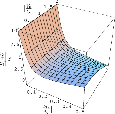
FIG. 2.: Phase diagram region where the presented ground-state solution occurs. The anisotropy parameter is $\chi=1.5$ and the relation $|V_{0}/V_{x}|=1/(2|t|)$ with $t=t_{2{\bf x}}/t_{\bf x}$ must also hold. For $t\to 0$ the presented surface extends along the $z=(E_{f}+U)/|t_{\bf x}|$ axis to $z\to\infty$.

FIG. 3.: Momentum distribution function $n({\bf k})=\langle\hat{C}^{\dagger}_{1,{\bf k},\sigma}\hat{C}_{1,{\bf k},\sigma}\rangle$ for the upper half filled diagonalized band, taken over the whole first Brillouin zone.

REFERENCES

- [1] Zs. Gulácsi, R. Starck, D. Vollhardt, Phys. Rev. B. 47, 8594, (1993).
- [2] M. A. N. Araujo, N. M. R. Peres, P. D. Sacramento, Phys. Rev. B. 65, 012503, (2001).
- [3] F. J. Ohkawa, Phys. Rev. B. 59, 8930, (1999).
- [4] U. Brandt, A. Giesekus, Phys. Rev. Lett. 68, 2648, (1992).
- [5] R. Strack, Phys. Rev. Lett. 70, 833, (1993).
- [6] I. Orlik, Zs. Gulácsi, Phil. Mag. B. 76, 845, (1997).
- [7] I. Orlik, Zs. Gulácsi, Phil. Mag. Lett. 78, 177, (1998).
- [8] Zs. Gulacsi, I. Orlik, J. Phys. A.Lett. 34, L359, (2001).
- [9] I. Orlik, Zs. Gulácsi, Phil. Mag. B. 81, 1587, (2001).
- [10] P. Gurin, Zs. Gulacsi, Phys. Rev. B. 64, 045118, (2001) and ibid. B. 65, 129901(E), (2002).
- [11] Zs. Gulácsi, Phys. Rev. B. 66, 165109, (2002).
- [12] Zs. Gulácsi, proceedings SCES-2002: Acta Phys. Polon. B. 34, 749, (2003).
- [13] A. J. Arko et al., Phys. Rev. B. 62, 1773, (2000).
- [14] A. J. Arko et al., J. Elec. Spec. 117-118, 323, (2001).
- [15] K. Held, R. Bulla, Eur. Phys. J. B. 17, 7, (2000).
- [16] K. Held et al. Phys. Rev. Lett. 85, 373, (2000).
- [17] C. Huscroft, A. K. McMahan, R. T. Scalettar, Phys. Rev. Lett. 82, 2342, (1999).
- [18] K. Held, A. K. McMahan, R. T. Scalettar, Phys. Rev. Lett. 87, 276404, (2001).
- [19] M. B. Zölfl, I. A. Nekrasov, Th. Pruschke, V. I. Anisimov, J. Keller, Phys. Rev. Lett. 64, 276403, (2001).
- [20] P. van Dongen et al. Phys. Rev. B. 64,195123, (2001).
- [21] H. L. Schläfer, G. Gliemann, Einführung in die Ligandenfeldtheorie, Akademische Verlagsgesellschaft, Frankfurt 1980, pg. 451 and tables on pg. 315-317.
- [22] R. B. Laughlin, G. G. Lonzarich, P. Monthoux, D. Pines, Advances in Phys. 50, 361, (2001).
- [23] R. Monnier, L. Degiorgi and D. D. Koelin, Phys. Rev. Lett. 56, 2744, (1986)