On the Rapid Increase of Intermittency in the Near-Dissipation Range of Fully Developed Turbulence

Abstract

Intermittency, measured as $\log\left({F(r)}/{3}\right)$, where $F(r)$ is the flatness of velocity increments at scale $r$, is found to rapidly increase as viscous effects intensify, and eventually saturate at very small scales. This feature defines a finite intermediate range of scales between the inertial and dissipation ranges, that we shall call near-dissipation range. It is argued that intermittency is multiplied by a universal factor, independent of the Reynolds number $Re$, throughout the near-dissipation range. The (logarithmic) extension of the near-dissipation range varies as $\sqrt{\log Re}$. As a consequence, scaling properties of velocity increments in the near-dissipation range strongly depend on the Reynolds number.

1 Introduction

Statistics of developed turbulence are commonly investigated by means of (longitudinal) velocity increments $\delta v(r)$ across a distance, or scale, $r$. At $r\approx L_{0}$, where $L_{0}$ represents the characteristic scale of the stirring forces (the integral scale of turbulence), fluid motions are statistically independent and the probability density function (pdf) of $\delta v(L_{0})$ is found nearly Gaussian. At smaller scales, intrinsic non-linear fluid dynamics operate and turbulent motions become intermittent; fluid activity comes in intense locally-organized motions embedded in a sea of relatively quiescent and disordered eddies (see meneguzzi ; orszag for first numerical indications). As a consequence, the pdf of $\delta v(r)$ develops long tails and becomes strongly non-Gaussian. Deviations from the Gaussian shape may be quantified by the flatness, defined as

$$F(r)\equiv\frac{\langle\delta v(r)^{4}\rangle}{\langle\delta v(r)^{2}\rangle^{2}}\mbox{ .}$$

For a centered Gaussian distribution $F=3$; as long tails develop $F$ increases. $F(r)/3$ may therefore be roughly thought of as the ratio of intense to quiescent fluid motions at scale $r$. In that sense, we shall assume in the following that $\log\left({F(r)}/{3}\right)$ provides a quantitative measure of intermittency morf .

The normalized (to the Gaussian value) flatness is plotted as a function of the scale ratio ${r}/{L_{0}}$ for two turbulent flows in Fig. 1. Experimentally, a particular attention has been paid to the size of the hot-wire probe and to the signal-to-noise ratio; small-scale velocity fluctuations are expected to be suitably resolved helium . The “instantaneous Taylor hypothesis” (see PinTaylor for details) has been used to estimate spatial velocity increments and reduce modulation effects morf ; helium . Details about the (standard) numerical integration of the Navier-Stokes equations can be found in numeric . We observe at scales $r\geq L_{0}$, $F(r)\simeq 3$, in agreement with the picture of disordered fluid motions: There is no intermittency, since the flatness $F(r)$ is independent of the scale $r$ and (almost) equal to the Gaussian value $F=3$. At smaller scales, $F(r)$ displays a power-law dependence on $r$: Intermittency grows up linearly with $\log(1/r)$. This scaling behavior is inherent to the inertial (non-linear) fluid dynamics and refers to the so-called inertial range. The exponent $\zeta_{F}\simeq-0.1$ is found very consistent with already reported values for homogeneous and isotropic turbulence scalings . Interestingly, $F(r)$ exhibits a rapid increase as viscous effects intensify, and eventually saturates at very small scales. This rapid increase of intermittency, which occurs over a range of scales that we shall call the near-dissipation range, is the main concern of this article. We shall here argue how intermittency in the near-dissipation range is related to the build-up of intermittency in the inertial range; the Reynolds-number dependence of this phenomenon will be also addressed.

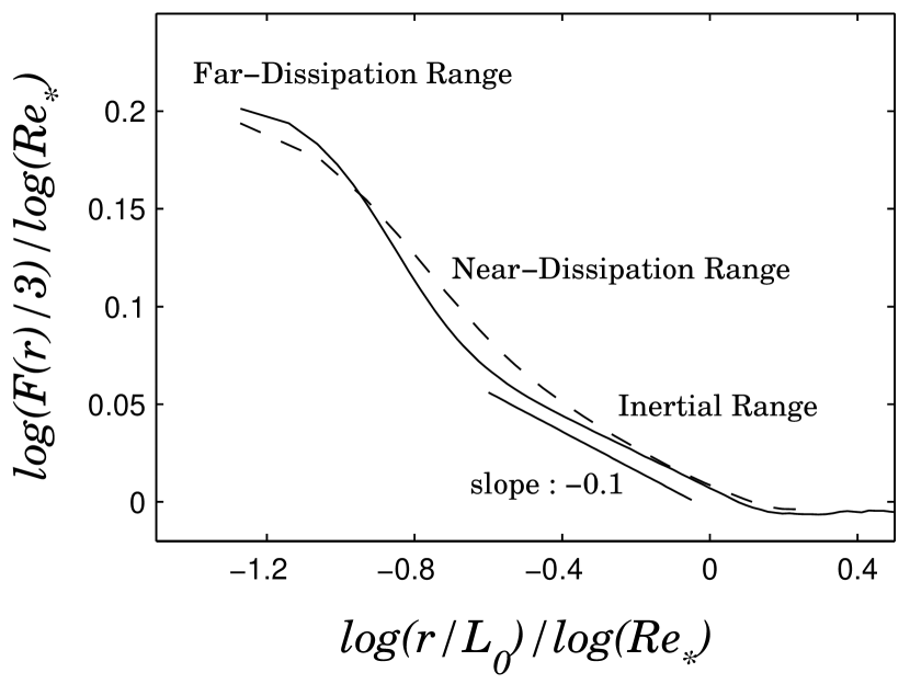
Figure 1: Scale dependence of the flatness of longitudinal velocity increments for two different turbulent flows: (solid line) a turbulent jet ($R_{\lambda}=380$) baudet and (dashed line) a direct numerical simulation ($R_{\lambda}=140$) numeric . The control parameter $Re_{*}$ is defined as $Re/R_{*}$, where $Re$ denotes the (usual) Reynolds number; the empirical constant $R_{*}\approx 56$ gagne ; lohse . Appendix A is devoted to the (modified) Reynolds number $Re_{*}$.

There has been a considerable amount of works on intermittency in the inertial range (see frisch for a review). Dissipation-range intermittency has received much less attention. In 1967, Kraichnan conjectured “unlimited intermittency” for the modulus of velocity Fourier modes at very high wavenumbers kraichnan . Although no proof was explicitly established for the Navier-Stokes equations, Frisch and Morf provided in 1981 strong mathematical arguments (occurrence of complex-time singularities) morf in support of Kraichnan’s conjecture. Following a previous study carried out by Paladin and Vulpiani in 1987 paladin , Frisch and Vergassola suggested in 1991 that multifractal (local) exponents $h$ of velocity increments, $\delta v(r)\sim r^{h}$, are successively turned-off as viscous effects intensify vergassola : As the scale $r$ decreases, only the strongest fluctuations (low $h$) survive while the others are extinguished by the viscosity. This mechanism reinforces the contrast between intense and quiescent motions, and thus provides a phenomenological explanation for the increase of intermittency in the near-dissipation range. However, as the remaining intense motions concentrate on a smaller and smaller fraction of the volume, this approach again predicts “unlimited intermittency” for the velocity increments $\delta v(r)$, in the limit of vanishing scale $r$.

As mentioned above, our experimental and numerical data indicate that intermittency, measured by the flatness of velocity increments, does exhibit a blow up in the beginning of the dissipation range but eventually saturates in the far-dissipation range. At this point, it should be mentioned that a spurious limitation of intermittency may stem from a lack of accuracy (or resolution) in velocity measurements or numerical simulations. However, a special care has been taken here to reduce this effect helium . In the following, we will argue that the observed saturation of intermittency is not an artefact, but refers to some peculiar properties of turbulence at very small, dissipative scales.

2 A multiplicative cascade description of intermittency

In the present study, the issue of intermittency in the dissipation range is reconsidered. The saturation of the flatness in the limit of vanishing scale $r$ is recovered by assuming that the velocity field is smooth (regular) in quiescent-flow regions (as already suggested in nelkin ; meneveau ): $\delta v(r)$ is not zero but behaves as $r$ in these regions; $\delta v(x,r)\approx r\partial_{x}v(x)$. This key assumption is here recast in a multiplicative approach of velocity-increment statistics along scales, as brought forward by Castaing et al. in CasGag90 . We shall then demonstrate that it is possible to gain quantitative results, without ad hoc parameters, on dissipative-range intermittency: The amplification of intermittency in the near-dissipation range and the extension of the near-dissipation range are explicitly estimated as a function of the Reynolds number.

The build-up of intermittency along the whole range of excited scales is related to the distortion of the pdf of $\delta v(r)$. In order to account for this distortion, let us formally introduce a random independent multiplier $\beta({r}/{L_{0}})$, connecting the statistics of $\delta v(r)$ at scales $r$ and $L_{0}$:

$$\delta v(r)=\beta(\frac{r}{L_{0}})\times\delta v(L_{0})\quad\textrm{for }r\leq L_{0}~{}.$$ (1)

The integral scale $L_{0}$ is taken as the reference scale. Eq. (1) should be understood in the statistical sense, i.e., the pdf of $\delta v(r)$ equals the pdf of $\beta({r}/{L_{0}})\times\delta v(L_{0})$ (see AmbBro99 for a Markovian description). The multiplier $\beta({r}/{L_{0}})$ is considered as a positive random variable. This approach therefore restricts to $|\delta v(r)|$ or to the symmetric part of the pdf of $\delta v(r)$; the skewness effects are beyond the scope of the present description.

From Eq. (1), it can be established that

$$P_{r}(\delta v)=\int G_{r,L_{0}}(\log\beta)P_{L_{0}}(\frac{\delta v}{\beta})\frac{\textrm{d}\log\beta}{\beta}~{},$$

where $P_{r}$ and $G_{r,L_{0}}$ denote respectively the pdf of $\delta v(r)$ and of $\log\beta({r}/{L_{0}})$. The pdf of $\delta v(L_{0})$ may be considered as Gaussian, as mentioned in the introduction. Once $P_{L_{0}}$ is known, $P_{r}$ is fully determined by $G_{r,L_{0}}$.

The so-called propagator kernel $G_{r,L_{0}}$ helium ; CasGag90 ; arneodo ; delour is characterized by the whole set of coefficients $C_{n}({r}/{L_{0}})$, defined by the expansion

$$\langle(\beta(\frac{r}{L_{0}}))^{p}\rangle=\exp\left(\sum_{n=1}^{\infty}C_{n}(\frac{r}{L_{0}})\frac{p^{n}}{n!}\right)\quad\textrm{for all }p.$$ (2)

By construction, $C_{n}({r}/{L_{0}})$ is the n${}^{\textrm{th}}$-order cumulant of the random variable $\log\beta(r/L_{0})$. For our purpose, we shall only focus on the first two cumulants: The mean

$$C_{1}(\frac{r}{L_{0}})\equiv\langle\log\beta(\frac{r}{L_{0}})\rangle$$ (3)

and the variance

$$C_{2}(\frac{r}{L_{0}})\equiv\langle\log^{2}\beta(\frac{r}{L_{0}})\rangle-\langle\log\beta(\frac{r}{L_{0}})\rangle^{2}~{}.$$ (4)

Experimentally, higher-order cumulants of $\log\beta({r}/{L_{0}})$ are found very small compared to $C_{1}({r}/{L_{0}})$ and $C_{2}({r}/{L_{0}})$ arneodo ; delour . This motivates our main interest in the mean and variance of $\log\beta({r}/{L_{0}})$ PhDChev . However, the exact shape of the propagator kernel $G_{r,L_{0}}$ is not relevant for the following analysis: Our arguments apply to the mean and the variance but does not require $G_{r,L_{0}}$ being Gaussian. This point should be unambiguous. We shall demonstrate that considering the mean and the variance of $G_{r,L_{0}}$ is valuable in order to describe the amplification of intermittency in the near-dissipation range.

What can be said about $C_{1}({r}/{L_{0}})$ and $C_{2}({r}/{L_{0}})$? First of all, it is straightforward to get from Eq. (1) and Eq. (2):

$$\langle|\delta v(r)|^{p}\rangle=K_{p}\sigma^{p}\exp\left(\sum_{n=1}^{\infty}C_{n}(\frac{r}{L_{0}})\frac{p^{n}}{n!}\right)$$

by assuming that $\delta v(L_{0})$ is a zero-mean gaussian variable of variance $\sigma^{2}$ (i.e., $\langle|\delta v(L_{0})|^{p}\rangle=K_{p}\sigma^{p}$).

– In the inertial range,

$$\langle|\delta v(r)|^{p}\rangle=K_{p}\sigma^{p}\left(\frac{r}{L_{0}}\right)^{\zeta_{p}}\mbox{ .}$$ (5)

This is the postulate of universal power-law scalings frisch ; K41 . It follows that $C_{1}({r}/{L_{0}})$ and $C_{2}({r}/{L_{0}})$ behave as linear functions of $\log({r}/{L_{0}})$:

$$C_{1}(\frac{r}{L_{0}}) = c_{1}\log(\frac{r}{L_{0}})\quad\textrm{and}$$

$$C_{2}(\frac{r}{L_{0}}) = c_{2}\log(\frac{r}{L_{0}})\quad\textrm{in the inertial range,}$$ (6)

where $c_{1}$ and $c_{2}$ are universal constants arneodo . The departure from the Kolmogorov’s linear scaling law $\zeta_{p}={p}/{3}$ is directly related to $c_{2}<0$:

$$\zeta_{p}=c_{1}p+c_{2}\frac{p^{2}}{2}+\cdots$$

In our framework, the build-up of intermittency (along the inertial range) is related to the increasing width of $G_{r,L_{0}}$ with the decreasing scale $r$, stating that the second-order cumulant $C_{2}(r/L_{0})$ increases as $r$ decreases.

– In the far-dissipative range, velocity increments are proportional to the scale separation $r$, which leads to

$$C_{1}(\frac{r}{L_{0}}) = \log(\frac{r}{L_{0}})+C_{1}^{\mathrm{diss.}}\quad\textrm{and}$$

$$C_{2}(\frac{r}{L_{0}}) = C_{2}^{\mathrm{diss.}}\quad\textrm{in the far-dissipation range.}$$

The constants $C_{1}^{\mathrm{diss.}}$ and $C_{2}^{\mathrm{diss.}}$ a priori depend on the Reynolds number, here defined as

$$R_{e}=\frac{\sigma L_{0}}{\nu},$$ (7)

where $L_{0}$ is the integral scale pointed out by Eq. (6), $\sigma$ denotes the standard deviation of $\delta v({L_{0}})$ and $\nu$ is the kinematic molecular viscosity.

– Finally, the inertial-range and far-dissipation-range behaviors of $C_{1}({r}/{L_{0}})$ and $C_{2}({r}/{L_{0}})$ match in the near-dissipation range. We will see that this matching is (very) peculiar.

Figure 2: Sketch of the distortion of the pdf of $\log\beta({r}/{L_{0}})$ along scales $r$, respectively in the inertial, near-dissipation and far-dissipation ranges. The width of the pdf increases rapidly when crossing the near-dissipation range from right to left; with decreasing scale $r$.

3 The near-dissipation range

Following Paladin and Vulpiani paladin , one considers that viscous effects at a given scale $r$ only affect the fluctuations of $\delta v(r)$, for which the local Reynolds number is smaller than a certain constant $R_{*}$. In the classical phenomenology of turbulence $R_{*}$ is fixed to unity frisch , but for our purpose, $R_{*}$ is kept as an empirical constant.

In our multiplicative cascade framework, the previous hypothesis writes

$$\frac{\sigma\beta(\frac{r}{L_{0}})r}{\nu}\leq R_{*}\mbox{ .}$$

This condition is equivalent to

$$\beta(\frac{r}{L_{0}})Re_{*}\left(\frac{r}{L_{0}}\right)\leq 1\mbox{ ,}$$ (8)

where $Re_{*}$ denotes the (modified) Reynolds number

$$Re_{*}\equiv\frac{R_{e}}{R_{*}}\mbox{ .}$$ (9)

The subscript $*$ indicates that $R_{*}$ is not a priori equal to unity; this point is clarified in the Appendix A.

The propagator kernel $G_{r,L_{0}}$ is sketched in Fig. 2 for various scales $r$ (the integral scale $L_{0}$ is fixed) as a function of $\log(\beta Re_{*}{r}/{L_{0}})$: $G_{r,L_{0}}$ moves from right to left as the scale $r$ decreases. At a given scale $r$, fluctuations $\beta({r}/{L_{0}})$ which satisfy Eq. (8) undergo dissipative effects. As viscosity strongly depletes these affected fluctuations, a significant stretching of the left tail of $G_{r,L_{0}}$ is expected (see Fig. 2). Viscous effects then lead to a strong distortion of $G_{r,L_{0}}$; a significant increase of $C_{2}(r/L_{0})$ follows. This argument provides a qualitative explanation of the increase of intermittency due to (non-uniform) viscous effects. Within this picture, the near-dissipation range may be viewed as the range of scales $r$ marked by the entering of $G_{r,L_{0}}$ in the viscous domain, and the leaving of $G_{r,L_{0}}$ from the inertial domain (see also Fig. 3).

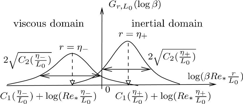
Figure 3: The near-dissipation range is given by $\eta_{-}<r<\eta_{+}$. The characteristic scales $\eta^{+}$ and $\eta^{-}$ are defined by Eqs. (10) and (11): The scale $\eta^{+}$ may be viewed as the smallest limiting scale for which the propagator $G_{r,L_{0}}$ is not affected by viscous effects; only non-linear dynamics prevail at $r>\eta^{+}$. The scale $\eta^{-}$ may be viewed as the largest limiting scale for which the propagator $G_{r,L_{0}}$ does not undergo non-linear effects; only viscous dynamics prevail at $r<\eta^{-}$.

In order to pursue a more quantitative analysis, an explicit definition of the near-dissipation range is required. To do so, let us introduce the two characteristic scales $\eta_{+}$ and $\eta_{-}$ (see Fig. 3) given respectively by

$$C_{1}(\frac{\eta_{+}}{L_{0}})+\log(Re_{*}\frac{\eta_{+}}{L_{0}}) = \sqrt{C_{2}(\frac{\eta_{+}}{L_{0}})}$$ (10)

$$\textrm{and}\quad C_{1}(\frac{\eta_{-}}{L_{0}})+\log(Re_{*}\frac{\eta_{-}}{L_{0}}) = -\sqrt{C_{2}(\frac{\eta_{-}}{L_{0}})}~{}.$$ (11)

According to our previous considerations, $\eta_{+}$ may be seen as the scale marking the entering of $G_{r,L_{0}}$ in the viscous domain, and $\eta_{-}$ as the scale marking the leaving of $G_{r,L_{0}}$ from the inertial domain. In other words, $\eta_{-}<r<\eta_{+}$ may be considered as the near-dissipation range; this will be our (explicit) definition.

It is natural to match the inertial-range and dissipation-range behaviors of $C_{1}({r}/{L_{0}})$ at the characteristic scale $\eta$, for which the propagator kernel, approximately centered around its mean value, extends equally over the inertial and viscous domains (see Figs. 2 and 3). This statement writes

$$\left<\log\left(\beta(\frac{\eta}{L_{0}})Re_{*}\left(\frac{\eta}{L_{0}}\right)\right)\right>=0\mbox{ ,}$$

and yields

$$C_{1}(\frac{\eta}{L_{0}})+\log(Re_{*}\frac{\eta}{L_{0}})=0\mbox{ .}$$

By assuming that the intermittency correction on $c_{1}$ is very small, so that $c_{1}\approx{1}/{3}$ according to Kolmogorov’s theory K41 , one obtains that $\eta$ coincides with the notorious Kolmogorov’s scale $\eta_{K}$, based on the modified Reynolds number $Re_{*}$:

$$\eta=\eta_{K}=L_{0}(Re_{*})^{-3/4}\mbox{ .}$$ (12)

Furthermore, $C_{1}^{\mathrm{diss.}}={1}/{2}\log Re_{*}$. From Eqs. (10), (11) and (12), it follows

$$\frac{\sqrt{C_{2}(\frac{\eta_{+}}{L_{0}})}}{\sqrt{C_{2}(\frac{\eta_{-}}{L_{0}})}}=\frac{\frac{4}{3}\log(\frac{\eta_{+}}{L_{0}})+\log Re_{*}}{-2\log(\frac{\eta_{-}}{L_{0}})-\frac{3}{2}\log Re_{*}}=\frac{\frac{4}{3}\log(\frac{\eta_{+}}{\eta})}{2\log(\frac{\eta}{\eta_{-}})}\mbox{ ,}$$

and by considering that $G_{\eta_{-},L_{0}}$ results from the distortion of $G_{\eta_{+},L_{0}}$, one obtains (see Appendix B for a kinematic proof)

$$2\sqrt{C_{2}(\frac{\eta_{+}}{L_{0}})}\approx\frac{4}{3}\log(\frac{\eta_{+}}{\eta_{-}})\mbox{ }$$ (13)

and

$$2\sqrt{C_{2}(\frac{\eta_{-}}{L_{0}})}\approx 2\log(\frac{\eta_{+}}{\eta_{-}})\mbox{ .}$$ (14)

These results finally yield $\log({\eta_{+}}/{\eta})=\log({\eta}/{\eta_{-}})$ and

$$\eta=\sqrt{\eta_{+}\eta_{-}}~{}.$$

In logarithmic coordinates the dissipative scale $\eta$, given by Eq. (12), lies at the center of the near-dissipation range: $\eta$ separates the inertial range and the far-dissipation range, as originally proposed by Kolmogorov. This is a first result concerning the near-dissipation range.

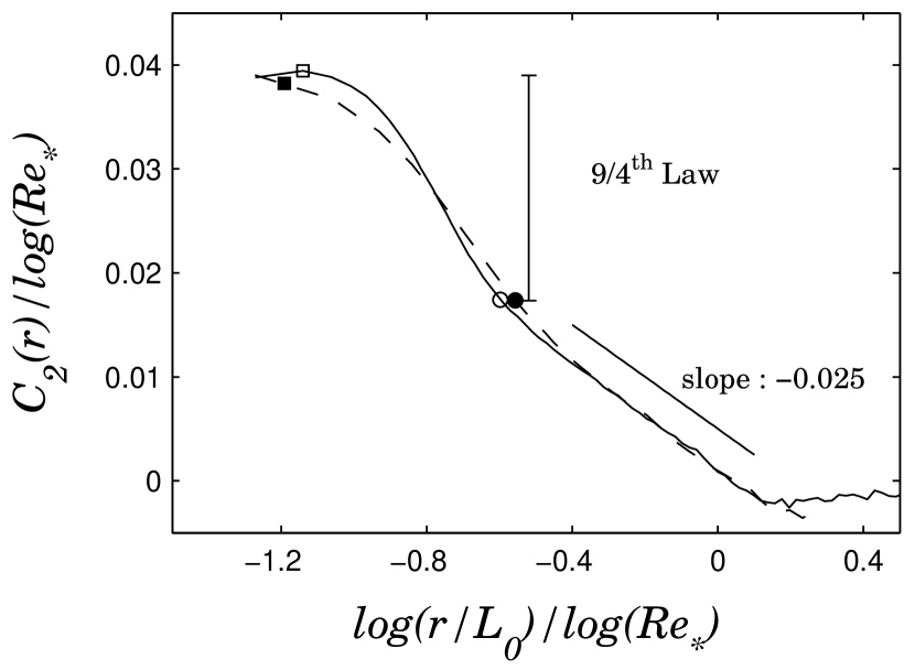
Figure 4: Scaling behavior of $C_{2}({r}/{L_{0}})$ for the turbulent jet and the numerical simulation. In the inertial range, $C_{2}(r)=c_{2}\log(r/L_{0})$ with $c_{2}\approx-0.025$. The two dissipative scales $\eta_{+}$ and $\eta_{-}$, defined by Eqs. (10) and (11), are indicated for both flows. The “amplification law” between $C_{2}({\eta_{-}}/{L_{0}})$ and $C_{2}({\eta_{+}}/{L_{0}})$ is very well satisfied. We observe also that the Kolmogorov’s dissipative scale $\eta$, given by Eq. (12), lies approximatively at the center of the near-dissipation range: $\eta_{-}<r<\eta_{+}$.

4 The amplification law

From the above computation, one can derive the “amplification law”

$${C_{2}(\frac{\eta_{-}}{L_{0}})}=\frac{9}{4}~{}{{C_{2}(\frac{\eta_{+}}{L_{0}})}}~{},$$ (15)

which characterizes the increase of intermittency in the near-dissipation range. The ${9}/{4}$ factor relies on the (reasonable) approximation that $c_{1}\approx{1}/{3}$. This does not mean at all that intermittency is ignored in our approach; it is just assumed here that the value of the parameter $c_{1}$, entering in the description, can be considered very close to its Kolmogorov value. Anyhow, the same reasoning could be pursued by keeping $c_{1}$ as a free parameter. In that case, the multiplicative factor would express as $4/(1+c_{1})^{2}$. Experimentally, one finds $c_{1}=0.37\pm 0.01$ CasGag90 .

Interestingly, the amplification of intermittency in the near-dissipation range is universal, independent of the (very high) Reynolds number. Let us also remark that this “amplification law” may serve as a useful benchmark for the (experimental or numerical) resolution of the finest velocity fluctuations; one should be able to differentiate (true) viscous damping and spurious filtering (see kadanoff for such a debate).

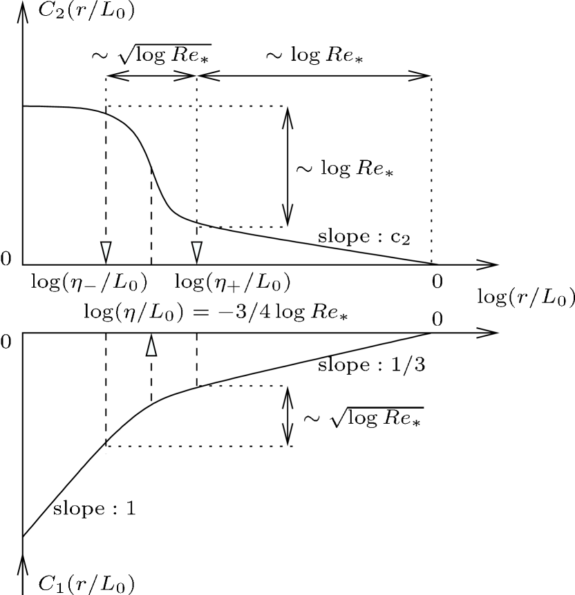
Figure 5: Sketch of the scaling behavior of $C_{1}({r}/{L_{0}})$ and $C_{2}({r}/{L_{0}})$ at high Reynolds number.

5 A unified picture of intermittency

At very high Reynolds number, $\sqrt{C_{2}({r}/{L_{0}})}$ becomes negligible compared to $\log Re_{*}$ in the near-dissipation range. It follows from Eqs. (10), (11) and the “amplification law” that $\eta_{+}\approx\eta_{-}\approx\eta$ at leading order in $\log Re_{*}$. This yields

$$C_{2}(\frac{\eta_{-}}{L_{0}})-C_{2}(\frac{\eta_{+}}{L_{0}}) \propto \log Re_{*}$$

$$\textrm{and}\quad C_{1}(\frac{\eta_{-}}{L_{0}})-C_{1}(\frac{\eta_{+}}{L_{0}}) \approx -\frac{2}{3}\log(\frac{\eta_{+}}{\eta_{-}})$$

$$\mathrm{with}\quad\log(\frac{\eta_{+}}{\eta_{-}}) \propto \sqrt{\log Re_{*}}~{}.$$ (16)

These behaviors are sketched in Fig. 5. One obtains that the (logarithmic) extension of the near-dissipation range ($\sim\sqrt{\log Re_{*}}$) becomes negligible compared to the extension of the inertial range ($\sim\log Re_{*}$). This is consistent with the tendency observed in Figs. 1 and 4. At this point, it should be emphasized that $\eta_{+}$ can not be assimilated to the Taylor’s microscale $\lambda$. Indeed, $\log(\eta_{+}/\eta)\propto\sqrt{\log Re_{*}}$ while on the contrary $\log(\lambda/\eta)\propto\log Re_{*}$.

Velocity increments follow a log-infinitely divisible law saito92 ; Nov94 in the inertial range, since all cumulants are proportional to a same function of the scale — $C_{p}({r}/{L_{0}})=c_{p}\log({r}/{L_{0}})$ for all $p$ — but this log-infinitely divisibility can not pertain in the near-dissipation range, according to the sketch in Fig. 5.

Intermittency has been related to $\log({F(r)}/{3})$ in the beginning. Using Eq. (1), one can derive the exact equation

$$\log\left(\frac{F(r)}{3}\right)=\sum_{p\geq 2}C_{p}(\frac{r}{L_{0}})\left(\frac{2^{2p}}{p!}-\frac{2^{p+1}}{p!}\right),$$ (17)

where $C_{p}({r}/{L_{0}})$ is the $p$-th order cumulant of $\log\beta({r}/{L_{0}})$. At leading order, this yields

$$\log\left(\frac{F(r)}{3}\right)=4C_{2}(\frac{r}{L_{0}})+\cdots,$$ (18)

which suggests that $\log({F(r)}/{3})$ and $C(r/L_{0})$ should behave in a very comparable way. Fig. 1 and Fig. 4 are indeed very similar. One may thus consider that $C_{2}({r}/{L_{0}})$ provides an alternative measure of intermittency, less intuitive than $\log\left({F(r)}/{3}\right)$ but physically more tractable (as demonstrated by this study). A specific test of Eq. (18) is provided in Fig. 6.

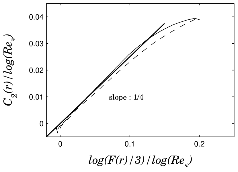
Figure 6: We observe that Eq. (18) is well satisfied in the inertial range (for the turbulent jet and the numerical simulation). A small departure is observed at small scales, when viscous effects intensify. This departure may be attributed to the growing of cumulants of order $p\geq 3$, neglected in Eq. (18).

Before concluding this study, let us mention that it is quite direct to generalize the previous analysis to $N$-order velocity increments:

$$\delta^{(1)}v(r)=v(x+r)-v(x),$$

$$\delta^{(2)}v(r)\equiv v(x+r)-2v(x+\frac{r}{2})+v(x),\quad\textrm{etc.}$$

Inertial-range scalings $\langle|\delta^{(N)}v(r)|^{p}\rangle\sim r^{\zeta_{p}}$ are preserved (as argued in arneodo ) but $\langle|\delta^{(N)}v(r)|^{p}\rangle\sim r^{Np}$ in the far-dissipative range. As a result, the definition of the near-dissipation is unchanged but the “amplification law” becomes

$${C_{2}^{(N)}(\frac{\eta_{-}}{L_{0}})}=\frac{9}{4}\left(\frac{(N+1)}{2}\right)^{2}{{C_{2}^{(N)}(\frac{\eta_{+}}{L_{0}})}}.$$ (19)

The amplification factor depends on the order $N$ of the velocity increment. This feature allows us to discriminate the inertial range and the near-dissipation range: Inertial-range scalings do not depend on $N$, while on the opposite, near-dissipation-range scalings depend drastically on $N$. Finally, the amplification factor in Eq. (19) diverges with $N$, tending toward Kraichnan’s view of unlimited intermittency (for the fluctuations of velocity Fourier modes) as $N\to\infty$ kraichnan .

6 Conclusion

A unified picture of velocity-increment intermittency, from the integral scale to the smallest (excited) scales of motion, is proposed. It is explicitly stated how far-dissipation range and inertial-range intermittencies match in the near-dissipation range. Especially, a universal “amplification law” determines how intermittency of velocity gradients is linked to the build-up of intermittency in the inertial range. The results are found in good agreement with our experimental and numerical observations.

Beyond these precise results, this study indicates that there are some peculiar and interesting physics around the Kolmogorov’s dissipative scale of turbulence. Such issue may be of great importance, for instance, in the modelling of mixing properties of turbulence, which mainly rely on the behavior of gradient fields chev_prl .

Finally, we would like to insist on the fact that this description leads to predictive results which could be used as tests for the suitable resolution of (very) small-scale fluctuations, to distinguish “probe effects” and true viscous damping. Relations between this study and the so-called property of Extended Self-Similarity ess should deserve some interests as well.

Appendix A The (modified) Reynolds number $Re_{*}$

The empirical constant $R_{*}$, which is abusively fixed to unity in the classical phenomenology of turbulence frisch , may be linked to the Kolmogorov’s constant $c_{K}$ (see yeungzhou and references therein).

In Kolmogorov’s 1941 theory, $c_{K}$ can be defined through the second-order velocity structure function:

$$\left<(\delta v(r))^{2}\right>=c_{K}\left<\epsilon\right>^{2/3}r^{2/3}\mbox{ ,}$$

where $\left<\epsilon\right>$ denotes the mean dissipation rate. Here, intermittency corrections are obviously omitted. By the use of Eq. (5), one can write

$$\langle(\delta v(r))^{2}\rangle=\sigma^{2}\left(\frac{r}{L_{0}}\right)^{2/3}\mbox{ ,}$$

which yields

$$c_{K}=\frac{\sigma^{2}}{\langle\epsilon\rangle^{2/3}L_{0}^{2/3}}\mbox{ .}$$ (20)

In this monofractal description, the near-dissipation range is degenerate and reduces to the Kolmogorov’s scale $\eta_{K}$. The second-order moment of velocity gradient expresses as

$$\left<(\partial_{x}v)^{2}\right>=\frac{\left<(\delta v(\eta_{K}))^{2}\right>}{(\eta_{K})^{2}}\mbox{ .}$$ (21)

By assuming homogeneous and isotropic turbulence, the mean dissipation rate writes $\langle\epsilon\rangle=15\nu\langle(\partial_{x}v)^{2}\rangle$. By combining the Eqs. (20) and (21), together with the definition of $\eta_{K}$ given by Eq. (12), one gets

$$c_{K}=\left(\frac{R_{*}}{15}\right)^{2/3}\quad\textrm{or}\quad R_{*}=15c_{K}^{3/2}\mbox{ .}$$ (22)

Eq. (22) indicates that $R_{*}$ is eventually much greater than unity. Following gagne , the empirical value $R_{*}\approx 56$ corresponds to $c_{K}\approx 2.4$. This value is in good agreement with experimental and numerical estimations $c_{K}\approx 2$ yeungzhou .

Appendix B Kinematic proof of Eqs. (13) and (14)

We provide a kinematic proof of Eqs. (13) and (14) with the help of Fig. 7:

— on the one hand, one derives from Eq. (10) that the distance

$$x_{A}-x_{A^{\prime}}=2\sqrt{C_{2}(\frac{\eta_{+}}{L_{0}})}~{}.$$

— on the other hand, the “position” of the point $M$, defined by the standard deviation around the mean, moves from $A$ to $A^{\prime}$ within the inertial domain (see Fig. 7) with a typical “velocity”

$$\frac{dx_{M}}{d\log{r/L_{0}}}\approx(c_{1}+1),$$

as $r$ decreases from $\eta_{+}$ to $\eta_{-}$. Within this representation (see PhDChev for details), the variable $\log{r/L_{0}}$ may be viewed as “time”. The correction due to the change of width of $G_{r,L_{0}}$ is neglected. Indeed, this correction expresses as $1/2\sqrt{c_{2}/\log(r/L_{0})}$ and can therefore be omitted in the near-dissipation range. One then gets

$$x_{A}-x_{A^{\prime}}\approx\frac{4}{3}\log(\frac{\eta_{+}}{\eta_{-}})\textrm{ by taking }c_{1}=\frac{1}{3}\mbox{ .}$$

Eq. (13) follows immediately. Eq. (14) can be demonstrated in a similar way by considering the motion of the point $M$ moving from $B$ to $B^{\prime}$ within the viscous domain.

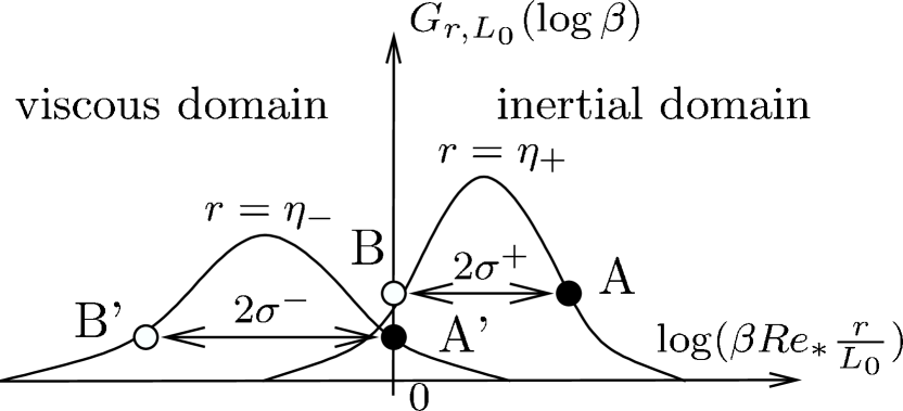
Figure 7: When the scale $r$ decreases, the propagator kernel $G_{r,L_{0}}$ moves from right to left ($\sigma$ denotes the standard deviation). At scale $r=\eta_{+}$, the points $A$ and $B$ are defined by the standard deviation around the mean. As $r$ decreases from $\eta_{+}$ to $\eta_{-}$, the points $A$ and $B$ move respectively to $A^{\prime}$ (within the inertial domain) and to $B^{\prime}$ (within the viscous domain).

References

- (1) A. Vincent and M. Meneguzzi, J. Fluid Mech. 225, (1991) 1-20
- (2) Z.-S. She, E. Jackson, and S. A. Orszag, Proc. R. Soc. London A 434, (1991) 101
- (3) U. Frisch, and R. Morf , Phys. Rev. A 23 (5), (1981) 2673
- (4) O. Chanal, B. Chabaud, B. Castaing, and B. Hébral, Eur. Phys. J. B 17, (2000) 301
- (5) J.-F. Pinton and R. Labbé, J. Phys. II France 4, (1994) 1461
- (6) E. Leveque and C. Koudella, Phys. Rev. Lett. 86, (2001) 4033
- (7) N. Cao, S. Chen, and Z.-S. She, Phys. Rev. Lett. 76, (1996) 3711
- (8) G. Ruiz-Chavarria, C. Baudet, and S. Ciliberto, Phys. Rev. Lett. 74, (1995) 1986
- (9) U. Frisch, Turbulence: the legacy of Kolmogorov, (Cambridge University Press, England, 1995)
- (10) B. Castaing, Y. Gagne, and M. Marchand, Physica D 68, (1993) 387
- (11) D. Lohse, Phys. Rev. Lett. 73 (24), (1994) 3223
- (12) R. H. Kraichnan, Phys. of Fluids 10, (1967) 2080
- (13) G. Paladin and A. Vulpiani, Phys. Rev. A 35, (1987) 1971
- (14) U. Frisch and M. Vergassola, Europhys. Lett. 14, (1991) 439
- (15) M. Nelkin, Phys. Rev. A 42(12), (1990) 7226
- (16) C. Meneveau, Phys. Rev. E 54, (1996) 3657
- (17) B. Castaing, Y. Gagne, and E. Hopfinger, Physica D 46, (1990) 177
- (18) P.-O. Amblard and J.-M. Brossier, Eur. Phys. J. B 12, (1999) 579
- (19) A. Arneodo, S. Manneville, and J.-F. Muzy, Eur. Phys. J. B 1, (1998) 129
- (20) J. Delour, J.-F. Muzy, and A. Arneodo, Eur. Phys. J. B 23, (2001) 243
- (21) L. Chevillard, PhD Thesis, Bordeaux I University, (2004) Available online at http://tel.ccsd.cnrs.fr
- (22) A. N. Kolmogorov, C. R. Acad. Sci. USSR 30, (1941) 301
- (23) V. Emsellem, L. P. Kadanoff, D. Lohse, P. Tabeling, and Z. J. Wang, Phys. Rev. E 55, (1997) 2672
- (24) Y. Saito, Phys. Soc. Japan 61, (1992) 403
- (25) E. A. Novikov, Phys. Rev. E 50, (1994) 3303
- (26) L. Chevillard, S. G. Roux, E. Leveque, N. Mordant, J.-F. Pinton, and A. Arneodo, Phys. Rev. Lett. 91, (2003) 214502
- (27) R. Benzi, S. Ciliberto, R. Tripiccione, C. Baudet, F. Massaioli, and S. Succi, Phys. Rev. E 48, (1993) R29
- (28) P. K. Yeung and Y. Zhou, Phys. Rev. E 56, (1997) 1746