Spin Projection Chromatography

Abstract

We formulate the many-body spin dynamics at high temperature within the non-equilibrium Keldysh formalism. For the simplest $XY$ interaction, analytical expressions in terms of the one particle solutions are obtained for linear and ring configurations. For small rings of even spin number, the group velocities of excitations depend on the parity of the total spin projection. This should enable a dynamical filtering of spin projections with a given parity i.e. a spin projection chromatography.

*corresponding author. E-mail address: horacio@famaf.unc.edu.ar (H. M. Pastawski)

PACS numbers:82.56.-b, 33.25.+k, 76.60.Lz

1 Introduction

The evolution of a local spin excitation in a system of interacting spins[1, 2] remains a problem of broad interest in theoretical and experimental physics. On one extreme, it seeks the quantification of the hydrodynamic limit of spin “diffusion” [3, 4]; on the other, the growing field of quantum information processing needs a dynamical[5, 6] control of individual spins in systems of intermediate size pushing the theory to its quantum limit. In spite of the naive expectation that quantum dynamical interferences might be limited to simple systems close to its ground state, most of the advances were originated on Nuclear Magnetic Resonance (NMR)[7] which deals with spin-spin interactions much weaker than the thermal energy $k_{B}T$. The discreteness of the spin system produces quantum beats that allow an efficient cross-polarization among different spin species[8]. In small bounded spin systems, such as molecules, the initial spreading out of a local excitation is followed by a revival known as Mesoscopic Echo[9] (ME) manifesting the reflection at the molecular boundaries. This echo was observed in the proton system of ferrocene[10], $\mathrm{(C_{5}H_{5})}_{2}\mathrm{Fe,}$ and benzene[11], $\mathrm{C}_{6}\mathrm{H}_{6}$, oriented molecules. Indeed, the complex interferences produced by the many-body dipolar interactions conspire against the spin wave behavior and produce a rapid attenuation of the ME. Therefore, a clean observation of the ME requires a reduction of the complex Heisenberg or Dipolar Hamiltonians to the simpler XY (Planar) Hamiltonian[12]. It is now clear, that even when one could control the many-body dynamics up to a high precision [13, 14], its intrinsic chaotic instability would easily degrade the quantum coherence[15]. This could explain the fast decay of the Magic Echoes[16], the Polarization Echoes [17, 18], and time reversal of cross-polarization[19] appearing when one “inverts” the sign of the effective many-spin Hamiltonian. ¿From this one learns that an attempt of dynamical control of many spins systems should focus in the simplest interactions. Spins arranged in a linear chain with XY interaction have a clearly non chaotic dynamics. This would enable the transfer of the polarization amplitude from one edge to any specified nucleus in the chain. Besides, as the field of quantum computing with NMR [20] grows steadily, one can foresee a new demand for alternatives to prepare and detect specific quantum states.

The aim of this letter is to propose a novel concept that we call spin projection chromatography. Given a collective spin excitation, it allows to filter out the components of a given total spin projection parity. To clarify the physics involved in this phenomenon, we use the known mapping between spins and fermions [21, 22] to develop a new formulation for spin dynamics based on the non-equilibrium formalism of Keldysh[23]. Its application to inhomogeneous chains and rings of spins 1/2 yields closed analytical expressions for the two site spin correlation functions that facilitate the prediction and understanding of interference phenomena in the spin dynamics at the molecular level.

2 Spin Dynamics in the Keldysh Formalism

The dynamics of a system with $M$ spins under a Hamiltonian $\mathcal{H}$ is usually described with the two site spin correlation function:

$$P_{f,i}(t)=\frac{\left\langle\Psi_{eq}\right|\widehat{S}_{f}^{z}(t)\widehat{S}_{i}^{z}(t_{0})\left|\Psi_{eq}\right\rangle}{\left\langle\Psi_{eq}\right|\widehat{S}_{i}^{z}(t_{0})\widehat{S}_{i}^{z}(t_{0})\left|\Psi_{eq}\right\rangle}.$$ (1)

This gives the amount of the $z$ component of the local polarization at time $t$ on site $f$-th, provided that the system was, at time $t_{0},$ in its equilibrium state with a spin “up” added at $i$-th site. Here, $\widehat{S}_{f}^{z}(t)=e^{\mathrm{i}\mathcal{H}t}\widehat{S}_{f}^{z}e^{-\mathrm{i}\mathcal{H}t}$ is the spin operator in the Heisenberg representation and $\left|\Psi_{eq}\right\rangle=\sum_{N}a_{N}\left|\Psi_{eq}^{(N)}\right\rangle$ is the thermodynamical many-body equilibrium state constructed by adding states with different number $N$ of spins up with appropriate statistical weights and random phases. The Jordan-Wigner (J-W) transformation [21] establishes the relation between spin 1/2 and fermion operators at site $n$,

$$\widehat{S}_{n}^{+}=\widehat{c}_{n}^{+}\exp\{\mathrm{i}\pi\sum_{m=1}^{n-1}\widehat{c}_{m}^{+}\widehat{c}_{m}\},$$

with $\widehat{c}_{m}^{+}$ and $\widehat{c}_{m},$ the creation and destruction operator for fermions, and $\widehat{S}_{n}^{\pm}$ the rising and lowering spin operator $\widehat{S}_{n}^{\pm}=\widehat{S}_{n}^{x}\pm\mathrm{i}\widehat{S}_{n}^{y}$, where $\widehat{S}_{n}^{\;u}$ ($u=x,y,z$) represents the Cartesian spin operator. The relation

$$\widehat{S}_{n}^{z}=\widehat{c}_{n}^{+}\widehat{c}_{n}-\tfrac{1}{2},$$

enables us to re-write the numerator of Eq. (1) as a density-density correlation:

$$\left\langle\Psi_{eq}\right|\widehat{S}_{f}^{z}(t)\widehat{S}_{i}^{z}(t_{0})\left|\Psi_{eq}\right\rangle=\left\langle\Psi_{eq}\right|[\widehat{c}_{f}^{+}(t)\widehat{c}_{f}(t)\widehat{c}_{i}^{+}(t_{0})\widehat{c}_{i}(t_{0})$$

$$-\tfrac{1}{2}\widehat{c}_{f}^{+}(t)\widehat{c}_{f}(t)-\tfrac{1}{2}\,\widehat{c}_{i}^{+}(t_{0})\widehat{c}_{i}(t_{0})+\tfrac{1}{4}]\left|\Psi_{eq}\right\rangle.$$ (2)

Since the last three terms in the rhs are constant occupation factors, the whole dynamics of the system is given by

$$\left\langle\Psi_{eq}\right|\widehat{c}_{f}^{+}(t)\widehat{c}_{f}(t)\widehat{c}_{i}^{+}(t_{0})\widehat{c}_{i}(t_{0})\left|\Psi_{eq}\right\rangle$$ (3)

$$=\sum_{N=0}^{M}\left|a_{N}\right|^{2}\sum_{\gamma=1}^{(\genfrac{}{}{0.0pt}{}{M}{N})}\left\langle\Psi_{\gamma}^{(N)}\right|\dfrac{\mathrm{e}^{-\beta\mathcal{H}}}{Z_{N}}\widehat{c}_{f}^{+}(t)\widehat{c}_{f}(t)\widehat{c}_{i}^{+}(t_{0})\widehat{c}_{i}(t_{0})\left|\Psi_{\gamma}^{(N)}\right\rangle.$$

Here, $\left|\Psi_{\gamma}^{(N)}\right\rangle$ and $Z_{N}$ are the many-body eigenstates and the partition function of the subspace with $N$ particles respectively. We have assumed the high temperature limit, $k_{B}T=\beta^{-1}\rightarrow\infty$ (i.e. $\mathrm{e}^{-\beta\mathcal{H}}\rightarrow I$), that leads to equal statistical weights $\left|a_{N}\right|^{2}=\frac{1}{2^{M}}\left(\genfrac{}{}{0.0pt}{}{M}{N}\right)$. Then, the invariance of the trace under cyclic permutations leads to:

$$\left\langle\Psi_{eq}\right|\widehat{c}_{f}^{+}(t)\widehat{c}_{f}(t)\widehat{c}_{i}^{+}(t_{0})\widehat{c}_{i}(t_{0})\left|\Psi_{eq}\right\rangle=\left\langle\Psi_{ne}\right|\widehat{c}_{f}^{+}(t)\widehat{c}_{f}(t)\left|\Psi_{ne}\right\rangle.$$ (4)

The state $\left|\Psi_{ne}\right\rangle\equiv\widehat{c}_{i}^{+}(t_{0})\left|\Psi_{eq}\right\rangle$ is a non-equilibrium many-body state generated at time $t_{0}$ by creating an excitation at site $i$. The operator $\widehat{c}_{f}^{+}(t)\widehat{c}_{f}(t)$ is evaluated over this non-equilibrium state. This is a particular case ($t_{1}=t_{2}=t$ and $k=l=f$) of the particle density function[23] in the Keldysh formalism:

$$G_{k,l}^{<}(t_{2},t_{1})=\tfrac{\mathrm{i}}{\hbar}\left\langle\Psi_{ne}\right|\widehat{c}_{k}^{+}(t_{1})\widehat{c}_{l}(t_{2})\left|\Psi_{ne}\right\rangle.$$ (5)

The two-time particle density is related to the exact retarded ($t_{2}>t_{1}$)  and advanced ($t_{2}<t_{1}$) Green’s functions of the many-body system,

$$G_{k,l}^{R}(t_{2},t_{1}) =[G_{l,k}^{A}(t_{1},t_{2})]^{\ast}$$ (6)

$$=-\tfrac{\mathrm{i}}{\hbar}\theta[t_{2}-t_{1}]\left\langle\Psi_{ne}\right|\widehat{c}_{k}(t_{2})\widehat{c}_{l}^{+}(t_{1})+\widehat{c}_{l}^{+}(t_{1})\widehat{c}_{k}(t_{2})\left|\Psi_{ne}\right\rangle,$$

which for quadratic Hamiltonians are just density conserving single particle propagators. In more complex cases, they can decay through the many-body or environmental interactions.

Both Eqs. (5) and (6) can be split out into the contribution of each subspace $N.$ In particular, the non-equilibrium initial density at $t_{0}$ describing an excitation at site $i$ is,

$$G_{k,l}^{<_{(N)}}(t_{0},t_{0})=\tfrac{\mathrm{i}}{\hbar}\left(\tfrac{N-1}{M-1}\delta_{k,l}+\tfrac{M-N}{M-1}\delta_{k,i}\delta_{i,l}\right),$$ (7)

a diagonal matrix involving equal weight for every site and an extra weight at the excited site $i$. In general, the initial state of Eq. (7) evolves under the Schrödinger equation expressed in the Danielewicz form [24, 25],

$$G_{f,f}^{\;<_{(N)}}(t,t)=\hbar^{2}\sum_{l,k}G_{f,k}^{R\,_{(N)}}(t,t_{0})G_{k,l}^{\;<_{(N)}}(t_{0},t_{0})G_{l,f}^{A_{(N)}}(t_{0},t)$$

$$+\sum_{l,k}\int_{t_{0}}^{t}\int_{t_{0}}^{t}G_{f,k}^{R_{(N)}}(t,t_{k})\Sigma_{k,l}^{<_{(N)}}(t_{k},t_{l})G_{l,f}^{A_{(N)}}(t_{l},t)\mathrm{d}t_{k}\mathrm{d}t_{l}.$$ (8)

The first term in the rhs can be seen as an integral form of the (reduced) density matrix ($\rho(t)=\mathrm{e}^{-\mathrm{i}\mathcal{H}t/\hbar}\rho(0)\mathrm{e}^{\mathrm{i}\mathcal{H}t/\hbar}$) projected over a basis of single particle excitations in its real space representation as previously used in related problems[26, 27, 28]. However, the second term would collect incoherent reinjections given by $\Sigma^{\;<}.$ These reinjection can compensate any eventual “leak” from the coherent evolution whenever the retarded and advanced propagators, $G^{R\,}$ and $G^{A\,},$ contain decoherent processes. They also can account for interactions that do not conserve spin projection. Notice that Eq. (8) gives the freedom to operate with two time indices $t_{k}$ and $t_{l},$ containing information about time correlations [25, 29, 30]. Hence, one could go beyond the standard initial value solution of the Schrödinger equation and include a continuous coherent injection of probability amplitude as is required to describe time dependent transport in mesoscopic and molecular devices[30, 31]. Future applications may include the descriptions of the chemical kinetics at low rates of laser pumping into the excited state[32, 33, 34] and the gradual creation of homonuclear coherence in NMR cross-polarization transfer [8].

Equation (8) allows the evaluation of Eq. (4) which gives the non-trivial dynamics of Eq. (1). Using the high temperature limit, $\left\langle\Psi_{eq}\right|\widehat{c}_{f}^{+}(t^{\prime})\widehat{c}_{f}(t^{\prime})\left|\Psi_{eq}\right\rangle\rightarrow$ $\frac{1}{2},$ the polarization is written as

$$P_{f,i}(t)=\sum_{N=1}^{M}\dfrac{\left(\genfrac{}{}{0.0pt}{1}{M-1}{N-1}\right)}{2^{M-1}}P_{f,i}^{(N)}(t),$$ (9)

with

$$P_{f,i}^{(N)}(t)=\tfrac{2\hbar}{\mathrm{i}}G_{f,f}^{<\,_{(N)}}(t,t)-1.$$ (10)

Here, the dynamics $P_{f,i}^{(N)}(t)$ of each subspace $N$, is weighted with the fraction of states that participate in the evolution.

We are now going to focus into systems where Eq. (8) takes the simplest form. If $\mathcal{H}$ commutes with the number operator, as is the case of the Heisenberg and truncated dipolar Hamiltonians, one is sure that different subspaces $N$ are decoupled. Further reduction could be obtained for Hamiltonians which are quadratic in the fermionic operator, such as the XY in proper conditions, as they might be reduced to non-interacting particles where $\Sigma_{k,l}^{\;<_{(N)}}\equiv 0$. Such cases have fully coherent evolution and enable the best manifestations of quantum interferences. Besides, these one-body solutions are needed to build up a decoherent perturbative approximation of the many-body dynamics.

3 Solution of Chains and Rings

Consider a linear chain of $M$ spins$-\frac{\mathrm{1}}{\mathrm{2}}$ in an external magnetic field and interacting with their nearest neighbors through an $XY$ coupling. Its Hamiltonian,

$$\widehat{\mathcal{H}}^{\mathrm{chain}}=\sum_{n=1}^{M}\hbar\Omega_{n}\left[\widehat{S}_{n}^{+}\widehat{S}_{n}^{-}-\tfrac{1}{2}\right]+\tfrac{1}{2}J_{n+1,n}(\widehat{S}_{n+1}^{+}\widehat{S}_{n}^{-}+\mathrm{c.c.}).$$ (11)

has a Zeeman part, $\widehat{\mathcal{H}}_{Z}$, proportional to $\widehat{S}_{n}^{z}$ with $\Omega_{n}$ the chemically shifted precession frequency; and a flip-flop term, $\widehat{\mathcal{H}}_{XY},$ where $J_{n,n+1}$ is the coupling between sites $n$ and $n+1$ with $J_{M,1}=0$.

Due to the short range interaction, after a J-W transformation the only non-zero coupling terms are proportional to $\widehat{c}_{n+1}^{+}\widehat{c}_{n}=\widehat{S}_{n+1}^{+}\widehat{S}_{n}^{-}$. Each subspace with $({\genfrac{}{}{0.0pt}{}{M}{N}})$ states of spin projection $\left\langle\sum_{n=1}^{M}\widehat{S}_{n}^{z}\right\rangle=N-M/2$ is now a subspace with $N$ non-interacting fermions. The eigenfunctions $\left|\Psi_{\gamma}^{(N)}\right\rangle$ are expressed as a single Slater determinant built-up with the single particle wave functions $\varphi_{\alpha}$ of energy $\varepsilon_{\alpha}$. Under this condition, $G_{f,i}^{R\,_{(N)}}(t)\equiv G_{f,i}^{R}(t)$ for every $N,$ and Eq. (9) reduces to

$$P_{f,i}^{\mathrm{chain}}(t)=\hbar^{2}\left|G_{f,i}^{R}(t)\right|^{2}.$$ (12)

Even for inhomogeneous systems, this can be solved analytically or numerically at low computational cost.

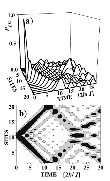
Figure 1: a) Evolution of the polarization at each site of a ring of size $M=20$ after a local excitation at site $10$. b) Contour plot of the polarization. Black filling represents $P>0.09;$ white is $P<0.045$ and grey corresponds to intermediate values.

For spins arranged in a ring, the closure of the chain requires an extra term in the Hamiltonian of Eq. 11, preventing the use of Eq. (12). After the J-W transformation this term takes the form ,

$$\tfrac{1}{2}J_{M,1}\widehat{S}_{1}^{+}\widehat{S}_{M}^{-}=-\tfrac{1}{2}J_{1,M}\widehat{c}_{1}^{+}\widehat{c}_{M}\exp[\mathrm{i}\pi\sum_{m=1}^{M}\widehat{c}_{m}^{+}\widehat{c}_{m}].$$ (13)

Thus the simple “flip-flop” interaction of the spin system becomes a “complex many-body” interaction term in the fermionic representation. The exponential can take the values $\pm 1$ depending on the parity of $N=\left\langle\Psi_{\gamma}^{(N)}\right|\widehat{N}$ $\left|\Psi_{\gamma}^{(N)}\right\rangle,$ the integer number of particles. Thus, there are two possible one-body Hamiltonians determining the wave functions $\varphi_{\alpha}(n)$ used to build the Slater determinant $\Psi_{\gamma}^{(N)}$. All subspaces with the same occupation parity are described with the same Hamiltonian. The different signs can be seen as a parity dependent boundary conditions (i.e. either periodic or antiperiodic) or even better as the effect of an effective potential vector $\mathbf{A}$, expressed in a singular gauge:

$$\mathrm{i}\pi\left[\sum_{m=1}^{M}\widehat{c}_{m}^{+}\widehat{c}_{m}\right]_{\operatorname{mod}2}=\mathrm{i}\frac{e}{\hbar}\int_{\mathbf{r}_{M}}^{\mathbf{r}_{1}}\mathbf{\mathbf{A}}\mathrm{d}\mathbf{\mathbf{l}}=\mathrm{i}\frac{e}{\hbar}{\displaystyle\oint}\mathbf{A}\mathrm{d}\mathbf{l=}\mathrm{i}2\pi\frac{\Phi}{\Phi_{0}}.$$ (14)

Here, the second equality defines the singular gauge for $\mathbf{A}$ which modifies the hopping term according to the Peierls substitution[35]. This results in an Aharonov-Bohm phase $2\pi\frac{\Phi}{\Phi_{0}},$ where $\Phi$ is the “fictitious” magnetic flux piercing the ring with value $\Phi=0$ or $\Phi=\frac{1}{2}\Phi_{0}=\frac{1}{2}h/e$ depending on the particle number (spin projection) parity. Therefore, an odd occupation ($N=2n+1$) yields $\Phi=0$, while the even occupation ($N=2n$ with $n$ integer) corresponds to $\Phi=\Phi_{0}/2$. The resulting Hamiltonian, expressed in the singular gauge and satisfying $\widehat{c}_{n}=\widehat{c}_{n+M}$, reads:

$$\widehat{\mathcal{H}}^{\mathrm{ring}}(\Phi)=\widehat{\mathcal{H}}^{\mathrm{chain}}+\tfrac{1}{2}(J_{1,M}\mathrm{e}^{\mathrm{i}2\pi\Phi/\Phi_{0}}\widehat{c}_{1}^{+}\widehat{c}_{M}+\mathrm{c.c.}).$$ (15)

The resulting propagators,

$$G_{f,i}^{R\,\,(2n+1)}(t) \equiv G_{f,i}^{R}(t;\Phi=0)~{}~{}\mathrm{and}$$ (16)

$$G_{f,i}^{R\,\,(2n)}(t) \equiv G_{f,i}^{R}(t;\tfrac{1}{2}\Phi_{0}),$$ (17)

are inserted in Eq. (8) to obtain the polarization from Eq. (9):

$$P_{f,i}^{\mathrm{ring}}(t)={\tfrac{\hbar^{2}}{2}}\left[\left|G_{f,i}^{R}(t;\Phi=0)\right|^{2}+\left|G_{f,i}^{R}(t;\Phi=\tfrac{1}{2}\Phi_{0})\right|^{2}\right].$$ (18)

Again, the dynamics is completely solved by evaluating the single particle Green’s functions.

4 Spin Projection and Excitation Velocities

Let us focus into the spin dynamics of homogeneous rings ($J_{n+1,n}\equiv J$ and $\Omega_{n}\equiv 0$). All the properties can be expressed in terms of the single particle wave-functions which we solve in the Coulomb gauge $\mathbf{A}=\frac{1}{2}\mathbf{B}\times\mathbf{r}$ obtaining $\varphi_{k}(n)=\left\langle 0\right|\widehat{c}_{n}\widehat{c}_{k}^{+}\left|0\right\rangle=\exp[\mathrm{i}\widetilde{k}n]/\sqrt{M}$; here $\left|0\right\rangle$ is the particle vacuum and $\widehat{c}_{k}^{+}$ creates a plane wave with a kinetic momentum $\hbar\widetilde{k}=\hbar k+\frac{\Phi}{\Phi_{0}}\frac{2\pi\hbar}{M}$ obtained from the stantard discrete wave vector given by $k=s2\pi/M$ with $s=1,\ldots M$; the lattice constant is $a\equiv 1$.  We recall that $\Phi$ is a fictitious flux identified with the parity of the number of spins up in the original problem. Hence, a high temperature excitation will require solutions with both fluxes $\Phi=0$ and $\Phi=\tfrac{1}{2}\Phi_{0}.$

Figure (1) shows the evolution of a local excitation through every site of a ring with $M=20$ sites at high temperature. The original excitation at the $10$-th site $G_{n,m}^{<}(t_{0},t_{0})=\frac{\mathrm{i}}{\hbar}\delta_{n,10}\delta_{10,m}$ splits-out into two wave packets with opposite velocities (i.e. + or -). Formally, $G_{n,m}^{<}(t,t)=G_{n,m}^{<(\mathrm{-})}(t,t)+G_{n,m}^{<(\mathrm{+})}(t,t)\,$where the partial particle densities propagate according to the definite sign in the kinetic momentum $\hbar\widetilde{k}.$ Let’s call $j_{n+1,n}(t)=j_{n}^{(\mathrm{+})}(t)-j_{n+1}^{(\mathrm{-})}(t)$ the current density between sites $n$ and $n+1.$ From Eq. (5.1) in Ref. [25] we get the partial currents:

$$j_{n}^{(\mathrm{\pm})}(t)=\tfrac{1}{2}J_{n,n+1}G_{n\pm 1,n}^{<(\mathrm{\pm})}(t,t)-\tfrac{1}{2}J_{n+1,n}G_{n,n\pm 1}^{<(\mathrm{\pm})}(t,t),$$ (19)

defining the propagation in each direction. The components with maximum velocity become increasingly dominant in the determination of the front of the wave packet. The eigenenergies $\varepsilon_{\widetilde{k}}=J\cos[\widetilde{k}]$ allow the evaluation of the group velocity $v_{\widetilde{k}}=\frac{1}{\hbar}\frac{\partial\varepsilon}{\partial\widetilde{k}}.$ The partial current and the corresponding local density can be used to evaluate the mean velocity as $\bar{v}=j/\rho,$ i.e.:

$$\overline{v}(\Phi,t)=\frac{\sum_{n}j_{n}^{(\mathrm{+})}(t)}{\sum_{n}\frac{\hbar}{\mathrm{i}}G_{n,n}^{<(\mathrm{+})}(t,t)}=\sum_{0\leq\widetilde{k}_{2}<\pi/a}\tfrac{2}{M}v_{\widetilde{k}_{2}},$$ (20)

setting a lower bound for the peak velocity. The revival time $T_{ME}$ for the mesoscopic echo is proportional to the ring size $M$ and inversely proportional to $\overline{v}$ and can be estimated as $M/v_{\mathrm{\max}}\leq T_{ME}<M/\overline{v}$. In Fig. (1b) the dominant group velocity manifests as a linear dependence of the wave packet maxima with time.

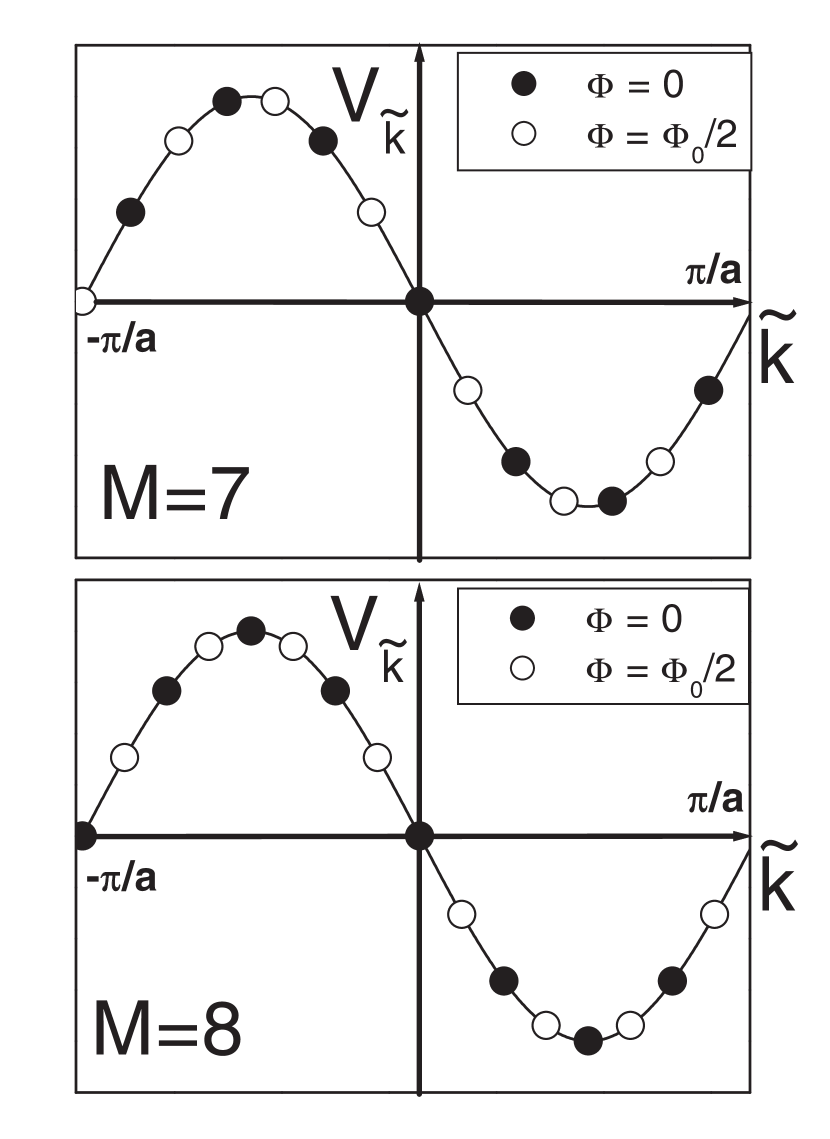
Figure 2: Dependence of velocities of eigenstates for rings with odd (7) and even (8) number of sites as function of the magnetic flux $\Phi$. Full and empty dots are eigenstates for the cases $\Phi=0$ and $\Phi=\Phi_{0}/2$ which corresponds to odd  and even total spin projection parity respectively. In rings with odd spin number parity the velocities do not depend on spin projection parity.

There is a fundamental difference between rings of odd and even number of sites $M.$ For odd sizes, the eigenstates determine the same set of velocities regardless of the boundary condition determined by the Aharonov-Bohm flux (which is half multiple of $\Phi=\Phi_{0}/2$ or $\Phi=0$). i.e. neither the available energies nor the velocities depend on the parity of the particle number, see the top of Fig. (2). However, the bottom panel shows that for even sizes, this symmetry is always absent and the set of velocities depend on $\Phi,$ i.e. on the parity of the particle number.

Different velocities for the eigenstates lead to different mean velocities for the localized excitation. Indeed, the evaluation of Eq. (20) for even values of $M$ yields

$$\overline{v}(\Phi)=\overline{v}(0)\cos(\frac{\Phi}{\Phi_{0}}\frac{2\pi}{M})-\frac{J}{\hbar}\frac{2}{M}\sin(\frac{\Phi}{\Phi_{0}}\frac{2\pi}{M}),$$

while for odd $M$ gives a mean velocity which does not depend on $\Phi$ (i.e. on the particle parity)

$$\overline{v}(\Phi)=\overline{v}(0),~{}~{}\text{with}~{}~{}\overline{v}(0)=-\frac{J}{\hbar}\frac{2}{M}/\tan(\frac{\pi}{M}).$$

It is evident that the mean velocity for the even ring sizes satisfies $\overline{v}(\Phi)>\overline{v}(0)$ indicating a faster propagation of the excitations with an even number of particles (i.e. in the subspace with even spin projection). For $M=8,$ $\overline{v}(\frac{1}{2}\Phi_{0})/\overline{v}(0)=1.08$, in contrast, for $M=7$ this ratio is $1$. This result is illustrated in Figure (3) for an $M=8$ spins system . Panel $a)$ shows the even ($\widehat{S}_{i}^{z(\mathrm{even})}=\sum_{n}\left\langle\Psi^{(2n)}\right|\widehat{S}_{i}^{z}\left|\Psi^{(2n)}\right\rangle$) and odd components of the local polarization for the ring with eight sites. Panel $b)$ shows the total polarization represented by the sum of both contributions. In summary, in rings with even number of spins an excitation in a subspace with even spin projection moves faster than one in a subspace with odd spin projection. This conclusion, easily derived in the language of “particles” and “fluxes”, would have been more elusive in the original language of spins. The novel concept revealed by the previous simple example is the possibility to manipulate collective entities as those constituted by the allowed total spin projections in a many-spin system.

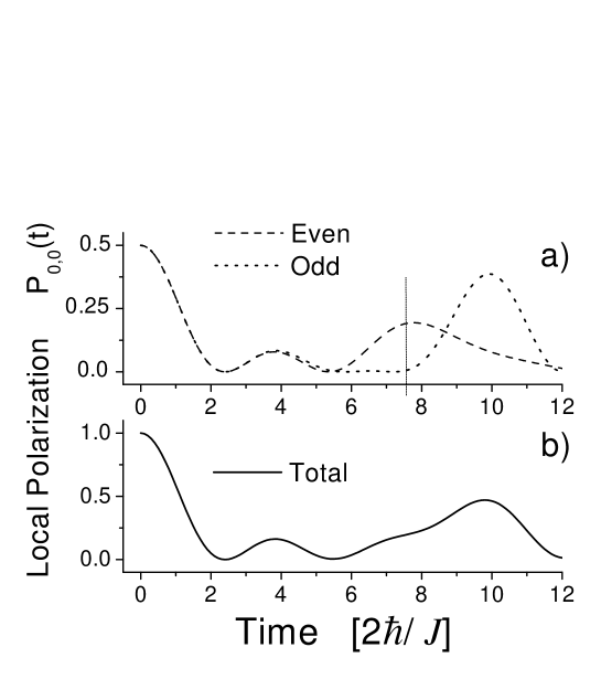
Figure 3: Spin Projection Chromatography in a ring with $M=8$. Panel $a)$ shows the contribution of even and odd spin projections to the local polarization, the sum of both, is shown in panel $b)$.

5 Conclusions

We must emphasize that the transparency of the formalism fully presented here for the first time, Eqs. (5-9), has already been instrumental to reveal the simple concepts hidden in the various problems related to spin dynamics such as the nature of Mesoscopic Echoes[9, 10] and Loschmidt Echoes [15].

The experimental realization of an $XY$ Hamiltonian can be achieved through the truncation of the more complicated Heisenberg (J-coupling) Hamiltonian by the pulse sequence developed in Ref. [12]. Its application to relatively small cyclic molecules of even parity (e.g. a derivative of octatetraene) would enable the observation of the described dynamics. The evident difference in the delay time of the ME of each spin projection allows one to manipulate them independently. One could conceive filtering out components of the total spin projection of a given parity. Consider a local magnetization (aligned in the $z$ direction) at a site distinguished by its chemical shift in the $M=8$ ring. This can be achieved by selective irradiation of one spin or by other polarization transfer method. This non-equilibrium initial state starts an evolution described by Eq. (18). After a time $T_{ME},$ the excitation will return to the initial site but the components moving in an even spin projection space will come back first. It is then possible to give a selective $\pi/2$-pulse (purification pulse) at $t=7.5(2\hbar/J),$ when the even spin projection has its maximum probability amplitude over the site and the corresponding probability amplitude for the odd spin projection is still close to cero, see Fig. (3). Thus, the even total spin projection has been tumbled down towards the $xy-$plane by the purification pulse leaving the odd one unaltered, i.e. an almost pure odd total spin projection state lies along the $z-$direction. Hence, the collective nature of the excitation can be used to achieve a dynamical filtering of the parity of the total spin allowing the purification of the desired component. This justifies the name of spin projection chromatography.

We acknowledge the financial support from ANPCyT, SeCyT-UNC, CONICET and Fundación Antorchas.

References

- [1] D. Foster, Hydrodynamic Fluctuations, Broken Symmetry and Correlation Functions, (Addison Wesley, Reading, MA 1990).
- [2] P. G. de Gennes, J. Phys. Chem. Solids 4 (1958) 223.
- [3] H. M. Pastawski and G. Usaj, Phys. Rev. B 57 (1998) 5017.
- [4] W. Zhang, and D. G. Cory, Phys. Rev. Lett. 80 (1998) 1324.
- [5] N. A. Gershenfeld and I. L. Chuang, Science 275 (1997) 350.
- [6] C. H. Bennett and D. P. Di Vincenzo, Nature 404 (2002) 247.
- [7] R. G. Brewer and E. Hahn, Sci. Am. 250(6) (1984) 50.
- [8] L. Müller, A. Kumar, T. Baumann, and R. R. Ernst, Phys. Rev. Lett. 32 (1974) 1402.
- [9] H. M. Pastawski, P. R. Levstein and G. Usaj, Phys. Rev. Lett. 75 (1995) 4310 .
- [10] H. M. Pastawski, G. Usaj, and P. R. Levstein, Chem. Phys. Lett. 261 (1997) 329.
- [11] A. K. Khitrin and B. M. Fung, J. Chem. Phys. 111 (1999) 7480.
- [12] Z. L. Mádi, B. Brutscher, T. Schulte-Herbrüggen, R. Brüschweiler and R. R. Ernst, Chem. Phys. Lett. 268 (1997) 300.
- [13] G. Usaj, H. M. Pastawski and P. R. Levstein, Mol. Phys. 95 (1998) 1229.
- [14] H. M. Pastawski, P. R. Levstein, G. Usaj, J. Raya and J. Hirschinger, Physica A 283 (2000) 166.
- [15] R. A. Jalabert and H. M. Pastawski, Phys. Rev. Lett. 86 (2001) 2490.
- [16] W. K. Rhim, A. Pines, and J. S. Waugh, Phys. Rev. Lett. 25 (1970) 218.
- [17] S. Zhang, B. H. Meier, and R. R. Ernst, Phys. Rev. Lett. 69 (1992) 2149.
- [18] P. R. Levstein, G. Usaj and H. M. Pastawski, J. Chem. Phys. 108 (1998) 2718.
- [19] M. Ernst, B. H. Meier, M. Tomaselli and A. Pines, Mol. Phys 95 (1998) 849.
- [20] C. Miquel, J. P. Paz, M. Saraceno, E. Knill, R. Laflamme, and C. Negrevergne, Nature 418 (2002) 62.
- [21] E. H. Lieb, T. Schultz, and D. C. Mattis, Ann Phys. 16 (1961) 407.
- [22] C. D. Batista and G. Ortiz, Phys. Rev. Lett. 86 (2001) 1082.
- [23] L. V. Keldysh, Zh. Eksp. Teor. Fiz. 47 (1964) 1515 [Sov. Phys.-JETP 20 (1965) 335].
- [24] P. Danielewicz, Ann. Phys. 152 (1984) 239.
- [25] H. M. Pastawski, Phys. Rev. B 46 (1992) 4053.
- [26] K. Schmidt-Rohr and H. W. Spiess, Multidimensional Solid-State NMR and Polymers, Academic Press (1996) Ch.3.
- [27] E. B. Fel’dman, R. Brüschweiler and R. R. Ernst, Chem. Phys. Lett. 294 (1998) 297.
- [28] E. B. Fel’dman and M. Rudavets, Chem. Phys. Lett. 311 (1999) 453.
- [29] H. M. Pastawski, Phys. Rev. B 44 (1991) 6329.
- [30] H. M. Pastawski, L. E. F. Foa Torres, and E. Medina, Chem. Phys. 281 (2002) 257.
- [31] A. P. Jauho, N. S. Wingreen and Y. Meir, Phys. Rev. B 50 (1994) 5528.
- [32] M. V. Ramakrishna and R. Coalson, Chem. Phys. 120 (1988) 327.
- [33] A. H. Zewail, J. Phys. Chem. A, 104 (2000) 5660.
- [34] H. van Willigen, P.R. Levstein and M. Ebersole, Chem. Rev. 93 (1993) 173.
- [35] R. P. Feynman, R. B Leighton and M. L. Sands, The Feynman Lectures on Physics, Vol III, Addison-Wesley (1989), Ch. 21.