Excitation lines and the breakdown of Stokes–Einstein relations in supercooled liquids

Abstract

By applying the concept of dynamical facilitation and analyzing the excitation lines that result from this facilitation, we investigate the origin of decoupling of transport coefficients in supercooled liquids. We illustrate our approach with two classes of models. One depicts diffusion in a strong glass former, and the other in a fragile glass former. At low temperatures, both models exhibit violation of the Stokes-Einstein relation, $D\sim\tau^{-1}$, where $D$ is the self diffusion constant and $\tau$ is the structural relaxation time. In the strong case, the violation is sensitive to dimensionality $d$, going as $D\sim\tau^{-2/3}$ for $d=1$, and as $D\sim\tau^{-0.95}$ for $d=3$. In the fragile case, however, we argue that dimensionality dependence is weak, and show that for $d=1$, $D\sim\tau^{-0.73}$. This scaling for the fragile case compares favorably with the results of a recent experimental study for a three-dimensional fragile glass former.

I Introduction

Normal liquids exhibit homogeneous behavior in their dynamical properties over length scales larger than the correlation length of density fluctuations. For example, the Stokes–Einstein relation that relates the self–diffusion constant $D$, viscosity $\eta$, and temperature $T$,

$$D\propto{T\over\eta},$$ (1)

is usually accurate Hansen and McDonald (1994); Balucani and Zoppi (1994). This relation is essentially a mean field result for the effects of a viscous environment on a tagged particle. In recent experimental studies, it has been reported that the Stokes–Einstein relation breaks down as the glass transition is approached in supercooled liquid systems Ediger (2000); Fujara et al. (1992); Chang and Sillescu (1997); Cicerone and Ediger (1996); Blackburn et al. (1996); Swallen et al. (2003). Translational diffusion shows an enhancement by orders of magnitude from what would be expected from Eq. (1) Hodgdon and Stillinger (1993); Stillinger and Hodgdon (1994); Tarjus and Kivelson (1995); Liu and Oppenheim (1996); Xia and Wolynes (2001). Here, we show that this breakdown is due to fluctuation dominance in the dynamics of low temperature glass formers. These pertinent fluctuations are dynamic heterogeneities Perera and Harrowell (1996, 1999, 1998); Kob et al. (1997); Donati et al. (1998, 1999a, 1999b); Glotzer (2000). Thus, the Stokes–Einstein breakdown is one further example of the intrinsic role of dynamic heterogeneity in structural glass formers Palmer et al. (1984); Garrahan and Chandler (2002, 2003).

In the treatment we apply, dynamic heterogeneity is a manifestation of excitation lines in space–time Garrahan and Chandler (2002). This picture leads to the prediction of dynamic scaling in supercooled liquids, $\tau(l)\sim l^{z}$. Here, $\tau(l)$ is the structural relaxation time for processes occurring at length scale $l$, and $z$ is a dynamic exponent for which specific results have been established Garrahan and Chandler (2002, 2003); Whitelam et al. (2003). This picture and its predicted scaling results differ markedly from those derived with the view that glass formation is a static or thermodynamic phenomenon Debenedetti and Stillinger (2001); Sastry et al. (1998); Büchner and Heuer (1999, 2000); Schroder et al. (2000); Keyes and Chowdhary (2002); Kivelson et al. (1995); Xia and Wolynes (2000). It also differs from mode coupling theory which predicts singular behavior at non–zero temperature Götze and Sjögren (1992); Kob (2003).

This paper is organized as follows. In Sec. II, we introduce our model for a supercooled liquid with a probe molecule immersed in the liquid. Simulation results are given in Secs. III and IV. Section IV also provides analytical analysis of the diffusion coefficient and the Stokes–Einstein violation, and explains the origin of the decoupling of transport coefficients based on the excitation line picture of trajectory space. Comparison of our theory with recent experimental results is carried out in Sec. V. We conclude in Sec. VI with a Discussion.

II Models

We imagine coarse graining a real molecular liquid over a microscopic time scale (e.g., larger than the molecular vibrational time scale), and also over a microscopic length scale (e.g., larger than the equilibrium correlation length). In its simplest form, we assume this coarse graining leads to a kinetically constrained model Garrahan and Chandler (2002, 2003); Fredrickson and Andersen (1984); Jäckle and Eisinger (1991); Ritort and Sollich (2003) with the dimensionless Hamiltonian,

$$H=\sum_{i=1}^{N}n_{i},\ \ (n_{i}=0,1).$$ (2)

Here, $n_{i}=1$ coincides with lattice site $i$ being a spatially unjammed region, while $n_{i}=0$ coincides with it being a jammed region. We call $n_{i}$ the “mobility field”. The number of sites, $N$, specifies the size of the system. From Eq. (2), thermodynamics is trivial, and the equilibrium concentration of defects or excitations is

$$c=\langle n_{i}\rangle={1\over 1+\exp({1/\widetilde{T}})},$$ (3)

where $\widetilde{T}$ is a reduced temperature. We make explicit connection of $\widetilde{T}$ with absolute temperature later when comparing our theory with experimental results.

The dynamics of these models obey detailed balance and local dynamical rules. Namely,

$$n_{i}=0\begin{array}[]{c}\xrightarrow{k_{i}^{(+)}}\\ \xleftarrow[k_{i}^{(-)}]{}\\ \end{array}n_{i}=1,$$ (4)

where the rate constants for site $i$, $k_{i}^{(+)}$ and $k_{i}^{(-)}$, depend on the configurations of nearest neighbors. For example, in dimension $d=1$,

$$k_{i}^{(+)} = e^{-1/\widetilde{T}}f(n_{i-1},n_{i+1}),$$ (5)

$$k_{i}^{(-)} = f(n_{i-1},n_{i+1}),$$ (6)

where $f(n_{i-1},n_{i+1})$ reflects the type of dynamical facilitation. In the Fredrickson–Andersen (FA) model Fredrickson and Andersen (1984), a state change is allowed when it is next to at least one defect. The facilitation function in this case is given by,

$$f_{\rm FA}(n_{i-1},n_{i+1})=n_{i-1}+n_{i+1}-n_{i-1}n_{i+1}.$$ (7)

In the East model Jäckle and Eisinger (1991), dynamical facilitation has directional persistence. The facilitation function in this case is

$$f_{\rm East}(n_{i-1},n_{i+1})=n_{i-1}.$$ (8)

In order to study translational diffusion in supercooled liquids, we extend the concept of dynamic facilitation to include a probe molecule. The dynamics of a probe will depend on the local state of the background liquid. When and where there is no mobility, the diffusive motion of the probe will be hindered. When and where there is mobility, the probe molecule will undergo diffusion easily. As such, in a coarse–grained picture, the probe molecule is allowed to jump from lattice site $i$ to a nearest neighbor site when site $i$ coincides with a mobile region, $n_{i}=1$. In order to satisfy detailed balance, we further assume that the probe molecule can move only to a mobile region, i.e.,

$$x(t+\delta t)=x(t)\pm\delta x\cdot n_{x}\cdot n_{x\pm\delta x},$$ (9)

where $x(t)$ denotes the position of the probe at time $t$. Units of time and length scales are set equal to a Monte Carlo sweep and a lattice spacing, respectively.

III Computer Simulations

Using the rules described in Sec. II, we have performed Monte Carlo simulations of diffusion of a probe molecule in the FA and East models for various temperatures. For the purpose of numerical efficiency, we have used the continuous time Monte Carlo algorithm Bortz et al. (1975); Newman and Barkema (1999). In the all systems, $N$ was chosen as $N=100/c$, and the simulations were performed for total times ${\cal T}\approx 100\tau$, with $\tau$ being the relaxation time of the model. Averages were performed over $10^{3}$ to $10^{5}$ independent trajectories.

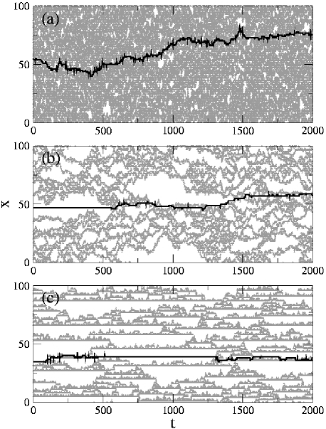
Figure 1: Typical trajectories of a probe molecule in one–dimensional models. The probe molecule (black line) undergoes a diffusive process in the trajectory space that consists of gray (mobile) and white (immobile) regions. (a) FA model at $\widetilde{T}=3$; (b) FA model at $\widetilde{T}=0.8$, and (c) East model at $\widetilde{T}=0.8$.

In Fig. 1, we show typical trajectories of probe molecules in the FA and East models. In the high temperature case, trajectory space is dense with mobile regions and there are no significant patterns in space–time. As such, the dynamics is mean–field like. It is for this reason that the relaxation time in this case is inversely proportional to the equilibrium probability of excitation, $c$ (see, for example, Ref. Berthier and Garrahan (2003a)). The probe molecule executes diffusive motion, without being trapped in immobile regions for any significant period of time.

The low temperature dynamics is different. Mobility is sparse, defects tend to be spatially isolated at a given time, and trajectory space exhibits space–time patterns. See Fig. 1(b) and (c). Because of the facilitation constraint, an immobile region needs a nearest mobile region to become mobile at a later time. The excitations therefore form continuous lines and bubble–like structures in trajectory space. While inside a bubble, the probe molecule will be immobilized. See, for example, the segment of the trajectory of a probe molecule for $0<t<500$ in Fig. 1(b). Due to exchanges between mobile and immobile regions, an immobile region can become mobile after a period of time. At that stage the probe molecule can perform a random walk until it is again in an immobile region. The motion of a probe molecule will manifest diffusive behavior over a time long enough for many dynamical exchanges to occur. In the East model at low temperatures such as pictured in Fig. 1(c), the bubbles in space–time form hierarchical structures Garrahan and Chandler (2002).

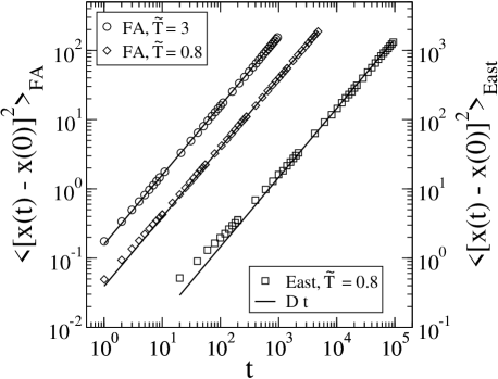
Figure 2: Mean squared displacements of the probe molecules are shown for the three different cases illustraed in Fig. 1.

Figure 2 plots mean square displacements of probe molecules for the FA and East models for three different cases pictured in Fig. 1. In the high temperature case, the mean square displacement reaches its diffusive linear regime after a very short transient time. In the low temperature case, the probe molecule in the East model case reaches the diffusive regime after a longer time and over a larger length scale than that in the FA model with the same reduced temperature.

IV Stokes–Einstein Violation

IV.1 Diffusion Coefficient

Figure 3 plots the diffusion coefficient of a probe molecule for the FA and the East models. The diffusion coefficient is determined from the mean square displacement,

$$D=\lim_{t\rightarrow\infty}{\langle[\Delta x(t)]^{2}\rangle\over t},$$ (10)

where $\Delta x(t)=x(t)-x(0)$. Error estimates for our simulations are no larger than the size of the symbols.

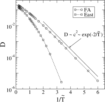
Figure 3: Diffusion coefficients for the FA and East models as functions of $1/\widetilde{T}$. Dashed lines are a guide to the eye.

In the FA model, the diffusion coefficient exhibits Arrhenius behavior for $\widetilde{T}<1$. This behavior reflects the fact that relaxation dynamics in the FA model is similar to that of a strong liquid. In this regime, over more than 4 orders of magnitude in $D$, the slope of $\log D$ vs $\widetilde{T}^{-1}$ is close to 2. This result is consistent with the expected low temperature scaling,

$$D_{\rm FA}\sim c^{2}\sim\exp(-2/\widetilde{T}),$$ (11)

as discussed in the next subsection. In the East model case, also pictured in Fig. 3, the diffusion coefficient decreases more quickly than Arrhenius. This super–Arrhenius behavior is due to the hierarchical nature of dynamics in the East model Sollich and Evans (1999).

Comparing the diffusion coefficients with the relaxation times of the background liquids demonstrates Stokes–Einstein violation in both models. The relaxation times, $\tau$, of the FA and the East models at different temperatures have been determined in prior work Buhot and Garrahan (2001); Berthier and Garrahan (2003b). When the Stokes–Einstein relation is satisfied, $D\tau\sim{\rm const}$. This behavior occurs in the FA and East models when $\tilde{T}>2$, but Fig. 4 shows that $D\tau$ is enhanced from that behavior by 2 or 3 orders of magnitude when $\tilde{T}<1$. Bear in mind, these deviations from Stokes–Einstein are $d=1$ results. The appropriate generalization of the FA model to $d=3$ does not exhibit such large deviations. On the other hand, we expect that generalizations of the East model, which is hierarchical and therefore fragile, will have weak dimensional dependence and continue to exhibit large deviations for $d=3$. We turn to the arguments that explain these claims now.

IV.2 Scaling Analysis

For high temperatures, the local mobility field will tend to be close to its mean value, $c$. As such, both the relaxation mechanism of the material and the diffusional motion of the probe molecule make use of the same local mobility fields. For this reason, the diffusion coefficient and the relaxation time scale are strongly coupled in this regime, leading to the Stokes–Einstein relation.

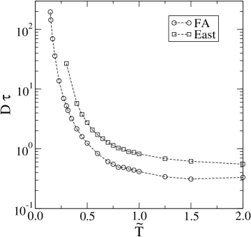
Figure 4: Violations of the Stokes–Einstein relation are similar in the $d=1$ FA and East models. Dashed lines are a guide to the eye.

At low temperatures, however, the dynamics of the system is not so simply related to the mean mobility field. Here, the fluctuations of bubble structures dominate. The relaxation time of the background liquid will approximately scale as the longest temporal extension of bubbles. The persistence time of an individual lattice site, $t_{\rm pers}$, is the time for which that site makes its first change in state. Its typical size will be intimately tied to the structural relaxation time of the liquid. For the FA model in $d=1$,

$$\tau\sim\langle t_{\rm pers}\rangle\sim c^{-3}.$$ (12)

See, for example, Refs. Ritort and Sollich (2003); Garrahan and Chandler (2002).

This result is consistent with a simple argument concerning diffusive motions of excitation lines in the low temperature FA model Garrahan and Chandler (2002). In particular, the structural relaxation times in the FA model is given by the time in which a typical bubble structure looses its identity through wandering motions of excitation lines. The excitation line has a local diffusivity of ${\cal D}\sim c$. (We use caligraphic ${\cal D}$ to distinguish this diffusion constant for excitations from that for particles, $D$.) In order to form a bubble, an excitation line needs to wander distance of the order of the typical length between defects, $l_{\rm eq}\sim c^{-1}$. Therefore, the mean relaxation time is given by $\tau\sim l_{\rm eq}^{2}/{\cal D}\sim c^{-3}$.

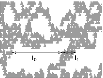
Figure 5: A section of Fig. 1(b) illustrating the meanings of exchange times, $t_{0}$ and $t_{1}$. $t_{0}$ is a time a site spends in a bubble, and $t_{1}$ is a time it spends in a surrounding boundary.

When the probe molecule is at the boundary of a bubble, it may not need to wait until the bubble closes in order to undergo diffusion; rather, it can remain within mobile cells and diffuse around the boundary of the bubbles. In this way, translational diffusion will be more facilitated than structural relaxation, leading to an enhanced diffusion in the fluctuation dominated low temperature region. Specifically, consider the dynamical exchange times, i.e., the times between flipping events for a given lattice site. See Fig. 5. $t_{0}$ is such a time duration for an $n_{i}=0$ state and $t_{1}$ is such a time duration for an $n_{i}=1$ state. The probe molecule can move only while in a mobile region. Further, the mean square displacement of the probe will be proportional to the number of diffusive steps that a probe molecule will take during the trajectory, ${\cal N}$,

$$\langle[\Delta x(t)]^{2}\rangle\sim{\cal{N}}\sim{{\cal T}\over\langle t_{0}\rangle+\langle t_{1}\rangle}.$$ (13)

Here, $\cal{T}$ is the length of a long trajectory in the FA model. The average duration of the defect state, $\langle t_{1}\rangle$, is inversely proportional to the probability of a lattice site being mobile, $c$, times the flip rate, $k_{i}^{(-)}$. Since $k_{i}^{(-)}\sim{\cal O}(1)$, we have,

$$\langle t_{1}\rangle\sim c^{-1}.$$ (14)

From detailed balance, therefore,

$$\langle t_{0}\rangle\sim c^{-2}.$$ (15)

Since $\langle t_{1}\rangle\ll\langle t_{0}\rangle$ in the low temperature region, Eqs. (13)–(15) give

$$D_{\rm FA}\sim{\langle(\Delta x)^{2}\rangle\over{\cal T}}\sim{1\over\langle t_{0}\rangle}\sim c^{2}.$$ (16)

This result explains Eq. (11). Together with Eq. (12), it leads to

$$D_{\rm FA}\sim\tau^{-\xi},$$ (17)

with $\xi=2/3$ in the $d=1$ FA model case. This scaling is to be contrasted with the Stokes–Einstein result, $\xi=1$.

Numerical simulation Garrahan and Chandler (2003) and renormalization group analysis Whitelam et al. (2003) of higher dimension generalizations of the FA model indicate that for $d=3$, $\tau\sim c^{-2.1}$. However, the scaling $D\sim c^{2}$ remains true for all dimensions as it is based solely on detailed balance. Thus, for $d=3$, $\xi\approx 0.95$. In other words, there is only a weak breakdown in the Stokes–Einstein relation for strong liquids in $d=3$.

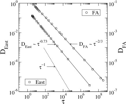
Figure 6: Scaling of Stokes–Einstein violation in $d=1$. Circles and squares indicate computed results for the FA and East models, respectively.

In the East model case, both the diffusion coefficient and the relaxation time show super-Arrhenius behavior. The hierarchical, fractal structure of pattern development in trajectory space for the East model does not allow a simple scaling analysis of the diffusion coefficient, and it is not obvious whether temperature independent scaling exists. One can define a temperature dependent scaling exponents, $\alpha(\widetilde{T})$ and $z(\widetilde{T})$,

$$D_{\rm East} \sim c^{\alpha(\widetilde{T})},$$ (18)

$$\tau \sim l^{z(\widetilde{T})},$$ (19)

so that

$$D_{\rm East}\sim\tau^{-{\alpha(\widetilde{T})/z(\widetilde{T})}}.$$ (20)

Interestingly, our numerical results indicate that $\xi={\alpha/z}\approx 0.73$ is independent of temperature as shown in Fig. 6. This exponent, $\xi\approx 0.73$ for the $d=1$ East model, is very close to what many experiments and simulations have found for three–dimensional glass forming liquids. For example, a recent experiment finds that $\xi\approx 0.77$ in the self–diffusion of tris-naphthylbenzene(TNB) Swallen et al. (2003). It was found that $\xi\approx 0.75$ in a molecular dynamics simulation of Lennard–Jones binary mixture Yamamoto and Onuki (1998) and a recent detailed scaling analysis of numerical results shows $\xi\approx 0.65$ Berthier (2003).

Presumably, such good agreement of scaling relation between the $d=1$ East model and higher dimension systems arises due to directional persistence of facilitation in the fragile liquid Garrahan and Chandler (2002, 2003). This persistence in higher dimensions causes motion to be effectively one–dimensional Garrahan and Chandler (2003). Therefore, dimensionality is not very significant for fragile glass formers. As such, for fragile systems, we expect that the scaling relation of the Stokes–Einstein violation will be reasonably well described by the $d=1$ East model. Based on this expectation, we further purse the comparison between theory and experiment.

V Comparison with Experiment

Swallen et al. Swallen et al. (2003) measured the self–translational diffusion coefficient of TNB near the glass transition temperature. They observed an increase of $D\eta/T$ from its high temperature limit by a factor of 400 near the glass transition temperature. In order to compare our results with these experiments, we need to determine the excitation concentration, $c$, as function of temperature. Since TNB behaves as a fragile liquid, we determine the excitation concentration as a function of temperature by fitting the viscosity data of TNB Plazek and Magill (1968) with the generalization of the East model formulas to higher dimensions Garrahan and Chandler (2003). Namely,

$$\ln{\tau}\approx{1\over d\ln 2}\left[\ln(g/c)\right]^{2},$$ (21)

where $g$ is the number of equally likely persistence directions on a cubic lattice, and

$$\ln(c)=\ln(c_{R})-J\left({1\over T}-{1\over T_{R}}\right).$$ (22)

The parameter $J$ is the energy scale associated with creating a mobile region from an immobile region, and $T_{R}$ is an appropriate reference temperature. Details on the fitting can be found in Ref. Garrahan and Chandler (2003). Taking $g=8$ (the cubic lattice value) and $T_{R}$ as the temperature at which $\log\tau$ is half the value of $\log\tau(T_{g})$, we determine that $J/T_{g}\approx 21.7$, and $\log_{10}(c_{R}/g)\approx-1.28$. The reduced temperature, $\widetilde{T}$ of the East model is related to absolute temperature by

$${1\over\widetilde{T}}=J\left({1\over T}-{1\over T_{R}}\right)+\ln(g/c_{R}).$$ (23)

Once we have determined the excitation concentration as a function of the temperature, we can compare experimental data with our computed results for the Stokes–Einstein violation in the East model case. Based on the argument that the scaling relation of the Stokes–Einstein violation ($D\sim\tau^{-\xi}$) remains robust in higher dimensions and from the dimensional dependence of Eq. (21), we expect

$$\ln{(D\tau)|_{d=3}}\approx{1\over 3}\ln{(D\tau)|_{d=1}}.$$ (24)

In Fig. 7 we use this relationship to compare the extent of the Stokes–Einstein violation of the experimental system with our East model results. The agreement between the two appears excellent.

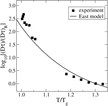
Figure 7: Comparison between the East model prediction and experiments on supercooled TNB, Ref. Swallen et al. (2003).

VI Discussion

There have been previous theoretical studies on the violation of the Stokes–Einstein relation in supercooled liquid systems. For example, Kivelson and Tarjus have argued that the Stokes–Einstein violation can be understood from their “frustration–limited domain” model for supercooled liquids Tarjus and Kivelson (1995); Kivelson et al. (1995). Assuming a distribution of local relaxation times associated with domain structures, this model describes the translational diffusion and viscosity as corresponding to different averaging process of such a distribution. Their idea contrasts to ours in that the domain structure in their work is purely static, and the exchange between different domains are not considered.

Hodgdon and Stillinger have proposed a fluidized domain model Hodgdon and Stillinger (1993); Stillinger and Hodgdon (1994). In their work, it is assumed that the system consists of a sparse collection of fluid–like domains in a background of more viscous media, and fluid–like domains appear and disappear with a finite life–time and rate. Relaxation times are determined by the rate of appearance of the fluid–like domains, while translation diffusion also depends on the life–time of the domains. To the extent that these domains refer to space–time and not simply space, this picture is not inconsistent with ours. Xia and Wolynes have applied the so–called “random first order transition theory” Xia and Wolynes (2000) to the Hodgdon–Stillinger model Xia and Wolynes (2001). In this case, the picture is both mean field and static and decidedly contrary to our fluctuation dominated and dynamic view.

From the perspective that Stokes–Einstein violation is a manifestation of fluctuation dominated dynamics, one expects that similar decoupling behavior occurs between other kinds of transport properties near the glass transition. The extent to which such decoupling can appear depends upon microscopic details in the specific transport properties and materials under study. For example, molecular rotations of a probe will be coupled to the mobility field, but less so than translations. Indeed, single molecule experiments indicate that rotations persist in both mobile and immobile regions of a glass former Deschenes and Bout (2001, 2002); Bartko et al. (2002). Rotational motions can therefore average the effects of dynamic heterogeneity to a greater extent than translational motions. As such, decoupling of rotational relaxation from structural relaxation can be more difficult to detect than violations of the Stokes–Einstein relation. Precisely how such effects might be detected seems worthy of further theoretical analysis.