Smeared phase transition in a three-dimensional Ising model with planar defects: Monte-Carlo simulations

Abstract

We present results of large-scale Monte Carlo simulations for a three-dimensional Ising model with short range interactions and planar defects, i.e., disorder perfectly correlated in two dimensions. We show that the phase transition in this system is smeared, i.e., there is no single critical temperature, but different parts of the system order at different temperatures. This is caused by effects similar to but stronger than Griffiths phenomena. In an infinite-size sample there is an exponentially small but finite probability to find an arbitrary large region devoid of impurities. Such a rare region can develop true long-range order while the bulk system is still in the disordered phase. We compute the thermodynamic magnetization and its finite-size effects, the local magnetization, and the probability distribution of the ordering temperatures for different samples. Our Monte-Carlo results are in good agreement with a recent theory based on extremal statistics.

I Introduction

The influence of disorder on a phase transition is an important and still partially open problem. Historically, the first attempts to address this question resulted in the belief that any kind of disorder would destroy a critical point because the system would divide itself into regions which independently undergo the phase transition at different temperatures. Therefore, there would not be a unique critical temperature for the system, but the phase transition would be smeared over an interval of temperatures. The singularities of thermodynamic quantities, which are the typical sign of a phase transition, would also be smeared (see Ref. Grinstein, 1985 and references therein).

However, it soon became clear that this belief was mistaken: in systems with weak short-range correlated disorder the phase transition remains sharp. Harris proposed a simple, heuristic criterionHarris (1974) for the influence of disorder on a critical point: if $\nu\geq 2/d$, where $\nu$ is the correlation length critical exponent and $d$ the spatial dimensionality, the disorder does not affect the critical behavior. In this case, the randomness decreases under coarse graining, and the system effectively looks homogeneous on large length scales. The critical behavior is identical to that of the clean system, i.e., the clean renormalization group fixed point is stable against disorder. The relative widths of the probability distributions of the macroscopic observables tend to zero in thermodynamic limit, i.e., they are self-averaging.

Even if the Harris criterion is violated the phase transition will generically remain sharp, but the critical behavior will be different from the clean case. There are two possible scenarios, a finite-randomness critical point or an infinite-randomness critical point. A critical point is of finite-randomness type if, under coarse graining, the system stays disordered on all length scales with the effective strength of the randomness approaching a finite constant. The probability distributions of thermodynamic observables reach a finite width in the thermodynamic limit, i.e., they are not self-averaging.Aharony and Harris (1996); Wiseman and Domany (1998) From a renormalization group point of view this means there is a critical fixed point with finite disorder strength. At a finite-randomness critical point, the thermodynamic observables obey standard power-law scaling behavior, but with exponents different from the exponents of the corresponding clean system. The other scenario, an infinite-randomness critical point, occurs if the effective disorder strength in the system grows without limit under coarse graining. The system looks more and more disordered on larger and larger length scales, i.e., it is described by a renormalization group fixed point with infinite disorder. The probability distributions of the thermodynamic observables become very broad (even on the logarithmic scale) and their widths diverge when approaching the critical point. The scaling behavior is of activated rather than of conventional power-law type. A famous example of an infinite-randomness critical point occurs in the McCoy-Wu model,McCoy and Wu (1968, 1969) a $2d$ Ising model with bond disorder perfectly correlated in one dimension and uncorrelated in the other. Recently, infinite-randomness critical points have also been found in several $1d$ random quantum spin chains and two-dimensional random quantum Ising models.Ma et al. (1979); Bhatt and Lee (1982); Fisher (1992, 1994, 1995); Young and Rieger (1996); Pich et al. (1998); Motrunich et al. (2000)

Disorder does not only influence the physics at the critical point itself, but also produces interesting effects close to it. These effects are known as Griffiths phenomena, a topic that has regained considerable attention in recent years. Griffiths phenomena are non-perturbative effects produced by rare disorder fluctuations close to a phase transition. They can be understood as follows: Generically, the critical temperature $T_{c}$ of a disordered system is lower than its clean value, $T_{c}^{0}$. In the temperature interval $T_{c}<T<T_{c}^{0}$, the bulk system is in the disordered phase. On the other hand, in an infinite size sample, there is an exponentially small, but finite probability for finding an arbitrary large region devoid of impurities. Such a region, a ’Griffiths island’, can develop local order while the bulk system is still disordered. Due to its size, such an island will have very slow dynamics because flipping it requires changing of the order parameter over a large volume, which is a slow process. GriffithsGriffiths (1965) showed that the presence of the locally ordered islands produces an essential singularityGriffiths (1965); Bray and Huifang (1989) in the free energy in the whole region $T_{c}<T<T_{c}^{0}$, which is now known as the Griffiths region or the Griffiths phase.Randeria et al. (1985) In generic classical systems the Griffiths singularity is weak, and it does not significantly contribute to the thermodynamic observables. In contrast, the long-time dynamics is dominated by these rare regions. Inside the Griffiths phase the spin autocorrelation function $C(t)$ decays as $\ln C(t)\sim-(\ln t)^{d/(d-1)}$ for Ising systemsRanderia et al. (1985); Dhar (1985); Dhar et al. (1988); Bray (1988); Bray and Rodgers (1988) and as $\ln C(t)\sim-t^{1/2}$ for Heisenberg systems.Bray (1988, 1987) These results were recently confirmed by more rigorous calculation for the equilibriumvon Dreyfus et al. (1995); Gielis and Maes (1995) and dynamicCesi et al. (1997a, b) properties of disordered Ising systems.

There are numerous systems where the disorder is not point like, but is realized through, e.g., dislocations or grain boundaries. This extended disorder in a $d$-dimensional system can often be modeled by defects perfectly correlated in $d_{C}$ dimensions and uncorrelated in the remaining $d_{\perp}=d-d_{C}$ dimensions. It is generally agreed that extended disorder will have even stronger effects on a phase transition than point-like impurities. Nevertheless, the fate of the transition in the presence of the extended impurities is not settled. Early renormalization group analysisLubensky (1975) based on a single expansion in $\epsilon=4-d$ did not produce a critical fixed point, leading to the conclusion that the phase transition is either smeared or of first order.Rudnick (1975); Andelman and Aharony (1975) Later workDorogovtsev (1980); Boyanovsky and Cardy (1982); Cesare (1994) which included an expansion in the number of correlated dimensions $d_{C}$ lead to a fixed point with conventional power law scaling. Subsequent Monte-Carlo simulations of a $3d$ Ising model with planar defects provided further support for a sharp phase transition scenario.Lee and Gibbs (1992) Notice, however, that the perturbative renormalization group calculations missed all effects coming form the rare regions. These effects were extensively studied for the above-mentioned McCoy-Wu model. While it was believed for a long time that the phase transition in this model is smeared, it was later found to be sharp, but of infinite-randomness type. McCoy (1969); Fisher (1992, 1995) Based on these findings, there was a general belief that a phase transition will remain sharp even in the presence of extended disorder.

Recently, it has been shown that this belief is not true. A theoryVojta (2003a, b) based on extremal statistics arguments has predicted that impurities correlated in a sufficiently high number of dimensions will generically smear the phase transition. The predictions of this theory were confirmed in simulations of mean-field type modelsVojta (2003a, b) but up to now, a demonstration of the smearing in a more realistic short-range model has been missing.

In this paper, we therefore present results of large-scale Monte-Carlo simulations for a $3d$ Ising model with planar defects and nearest-neighbor interactions in both the correlated and uncorrelated dimensions. These simulations show that the sharp phase transition is indeed destroyed by the extended disorder. The smearing of the transition is a consequence of a mechanism similar to but stronger than the Griffiths phenomena. In an Ising system with planar defects true static long-range order can develop on rare islands devoid of impurities. As a consequence, the order parameter becomes spatially very inhomogeneous and its average develops an exponential dependence on temperature. This paper is organized as follows. In section II, the model is introduced and the mechanism of the smearing is explained. Section III is devoted to the results of the Monte-Carlo simulations and a comparison with the theoretical predictions. In Section IV, we present our conclusions and discuss a number of open questions.

II The Model

II.1 3D Ising model with planar defects

Our starting point is a $3d$ Ising model with planar defects. Classical Ising spins $S_{ijk}=\pm 1$ reside on a cubic lattice. They interact via nearest-neighbor interactions. In the clean system all interactions are identical and have the value $J$. The defects are modeled via ’weak’ bonds randomly distributed in one dimension (uncorrelated direction). The bonds in the remaining two dimensions (correlated directions) remain equal to $J$. The system effectively consists of blocks separated by parallel planes of weak bonds. Thus, $d_{\bot}=1$ and $d_{C}=2$. The Hamiltonian of the system is given by:

$$H= -\sum_{{i=1,\dots,L_{\bot}}\atop{j,k=1,\dots,L_{C}}}J_{i}S_{i,j,k}S_{i+1,j,k}$$ (1)

$$-\sum_{{i=1,\dots,L_{\bot}}\atop{j,k=1,\dots,L_{C}}}J(S_{i,j,k}S_{i,j+1,k}+S_{i,j,k}S_{i,j,k+1}),$$

where $L_{\bot}$($L_{C}$) is the length in the uncorrelated (correlated) direction, $i$, $j$ and $k$ are integers counting the sites of the cubic lattice, $J$ is the coupling constant in the correlated directions and $J_{i}$ is the random coupling constant in the uncorrelated direction. The $J_{i}$ are drawn from a binary distribution:

$$J_{i}=\left\{\begin{array}[]{clc}cJ&\textrm{with probability}&p\\ J&\textrm{with probability}&1-p\end{array}\right.$$ (2)

characterized by the concentration $p$ and the relative strength $c$ of the weak bonds ($0<c\leq 1$). The fact that one can independently vary concentration and strength of the defects in an easy way is the main advantage of this binary disorder distribution. However, it also has unwanted consequences, viz. log-periodic oscillations of many observables as functions of the distance from the critical point.Karevski and Turban (1996) These oscillations are special to the binary distribution and unrelated to the smearing considered here; we will not discuss them further. The order parameter of the magnetic phase transition is the total magnetization:

$$m=\frac{1}{V}\sum_{i,j,k}\langle S_{i,j,k}\rangle,$$ (3)

where $V=L_{\bot}L_{C}^{2}$ is the volume of the system, and $\langle\cdot\rangle$ is the thermodynamic average.

Now we consider the effects of rare disorder fluctuations in the system. Similarly to the Griffiths phenomena, there is a small but finite probability to find a large spatial region containing only strong bonds in the uncorrelated direction. Such a rare region can locally be in the ordered state while the bulk system is still in the disordered (paramagnetic) phase. The ferromagnetic order on the largest rare regions starts to emerge right below the clean critical temperature $T_{c}^{0}$. Since the defects in the system are planar, these rare regions are infinite in the two correlated dimensions but finite in the uncorrelated direction. This makes a crucial difference compared to systems with uncorrelated disorder, where rare regions are of finite extension. In our system, each rare region is equivalent to a two dimensional Ising system that can undergo a real phase transition independently of the rest of the system. Thus, each rare region can independently develop true static order with a non-zero static value of the local magnetization. Once the static order has developed, the magnetizations of different rare regions can be aligned by an infinitesimally small interaction or external field. The resulting phase transition will thus be markedly different from a conventional continuous phase transition. At a conventional transition, a non-zero order parameter develops as a collective effect of the entire system which is signified by a diverging correlation length of the order parameter fluctuations at the critical point. In contrast, in a system with planar defects, different parts of the system (in the uncorrelated direction) will order independently, at different temperatures. Therefore the global order will develop inhomogeneously and the correlation length in the uncorrelated direction will remain finite at all temperatures. This defines a smeared transition. Thus we conclude that planar defects destroy a sharp phase transition and lead to its smearing.

II.2 Results of extremal statistics theory

In this subsection we briefly summarize the results of the extremal statistics theoryVojta (2003b) for the behavior in the ’tail’ of the smeared transition, i.e., in the parameter region where a few rare regions have developed static order but their density is still sufficiently low so they can be considered as independent. The approach is very similar to that of Lifshitz Lifshitz (1964) and others developed for the description of the tails in the electronic density of states. The extremal statistics theoryVojta (2003b) correctly describes the leading (exponential) behavior of the magnetization and other observables. A calculation of pre-exponential factors would be much more complicated because one would have to include, among other things, details of the geometry of the rare regions, surface critical behavior Binder (1983); Diehl (1986) at the surfaces of the rare regions, and corrections to finite-size scaling. This is beyond the scope of the present paper.

The probability $w$ to find a large region of linear size $L_{\bot}$ containing only strong bonds is, up to pre-exponential factors:

$$w\sim(1-p)^{L_{\bot}}=e^{\log(1-p)L_{\bot}}.$$ (4)

As discussed in subsection II.1, such a rare region develops static long-range (ferromagnetic) order at some reduced temperature $T_{c}(L_{\bot})$ below the clean critical reduced temperature $T_{c}^{0}$. The value of $T_{c}(L_{\bot})$ varies with the length of the rare region; the longest islands will develop long-rage order closest to the clean critical point. A rare region is equivalent to a slab of the clean system, we can thus use finite size scaling to obtain:

$$T_{c}^{0}-T_{c}(L)=|t_{c}(L)|=AL^{-\phi},$$ (5)

where $\phi$ is the finite-size scaling shift exponent of the clean system and A is the amplitude for the crossover from three dimensions to a slab geometry infinite in two (correlated) dimension but with finite length in the third (uncorrelated) direction. The reduced temperature $t=T-T_{c}^{0}$ measures the distance form the clean critical point. Since the clean 3$d$ Ising model is below its upper critical dimension ($d_{c}^{+}=4$), hyperscaling is valid and the finite-size shift exponent $\phi=1/\nu$. Combining (4) and (5) we get the probability for finding an island of length $L_{\bot}$ which becomes critical at some $t_{c}$ as:

$$\begin{array}[]{cc}w(t_{c})\sim e^{-B|t_{c}|^{-\nu}}&\textrm{(for $t_{c}\to 0-$)}\end{array}$$ (6)

with the constant $B=-\log(1-p)A^{\nu}$. The total (average) magnetization $m$ at some reduced temperature $t$ is obtained by integrating over all rare regions which have $t_{c}>t$. Since the functional dependence on $t$ of the local magnetization on the island is of power-law type it does not enter the leading exponentials but only pre-exponential factors, so:

$$\begin{array}[]{cc}m(t)\sim e^{-B|t|^{-\nu}}&\textrm{(for $t\to 0-$)}.\end{array}$$ (7)

Now we turn our attention to the homogeneous magnetic susceptibility. It contains two contributions, one coming from the islands on the verge of ordering and one from the bulk system still deep in the disordered phase. The bulk system provides a finite, non-critical background susceptibility throughout the whole tail region of the smeared transition. In order to estimate the second part of the susceptibility, i.e., the part coming from the islands consider the onset of local magnetization at the clean critical point. Using eq. (6) for the density of islands we can estimate:

$$\begin{array}[]{cc}\chi\sim\int_{0}^{\Lambda}dtt^{-\gamma}e^{-Bt^{-\nu}}&\textrm{(for $t\to 0-$)}.\end{array}$$ (8)

The last integral is finite because the exponentially decreasing island density overcomes the power-law divergence of the susceptibility of an individual island. Here $\gamma$ is the clean susceptibility exponent and $\Lambda$ is related to a lower cutoff for the island size. Once the first island is ordered it produces an effective background magnetic field which cuts off any possible divergence in $\chi$. Therefore, we conclude that the homogeneous magnetic susceptibility does not diverge anywhere in the tail of the smeared transition. However, there is an essential singularity at the clean critical temperature produced by the vanishing density of ordered islands. Because if this singularity one might be tempted to call this temperature the transition temperature of our system, but this is not appropriate because at this temperature only an infinitesimally small part of the system starts to develop a finite magnetization while most of the system remains solidly in the nonmagnetic phase. We rather view the clean critical temperature as the onset of the smearing region in our model.Vojta (2003b)

The spatial distribution of the magnetization in the tail region of the smeared transition is very inhomogeneous. On the already ordered islands, the local (layer) magnetization $m_{i}=(1/L_{C}^{2})\sum_{j,k}\langle S_{i,j,k}\rangle$ is comparable to the magnetization of the clean system. On the other hand, far away from the ordered islands $m_{i}$ decays exponentially with the distance from the closest one. The probability distribution of the logarithm of the magnetization $P[\log m_{i}]$ will therefore be very broad, ranging from $\log m_{i}=O(1)$ on the largest islands to $\log m_{t}\to-\infty$ on sites very far away from any ordered islands. The typical magnetization $m_{typ}$ can be estimated from the typical distance of a point from the nearest ordered island. Using eq. (6) we get:

$$x_{typ}\sim e^{B|t|^{-\nu}}.$$ (9)

At the distance $x_{typ}$ from an ordered island, the local magnetization has decayed to

$$m_{typ}\sim e^{-x_{typ}/\xi_{0}}\sim e^{-Ce^{B|t|^{-\nu}}}$$ (10)

where $\xi_{0}$ is the bulk correlation length, which is finite and changes slowly throughout the tail region of the smeared transition, and $C$ is a constant. A comparison with eq. (7) gives the relation between $m_{typ}$ and the thermodynamic order parameter (magnetization) $m$ as:

$$|\log m_{typ}|\sim\frac{1}{m}.$$ (11)

Thus, $m_{typ}$ decays exponentially with $m$ indicating an extremely broad order parameter distribution. In order to determine the functional form of the local order parameter distribution, first consider a situation with just a single ordered island at the origin of the coordinate system. For large distances $x$, the local magnetization falls off exponentially as $m(x)=m_{0}~{}e^{-x/\xi_{0}}$. The probability distribution of $y=\log[m(x)]=\log m_{0}-x/\xi_{0}$ can be calculated from

$$P(|y|)=\left|\frac{dN}{dy}\right|=\frac{dN}{dx}\left|\frac{dx}{dy}\right|=\xi_{0}\frac{dN}{dx}\sim\xi_{0}$$ (12)

where $dN$ is the number of sites at a distance from the origin between $x$ and $x+dx$ or, equivalently, having a logarithm of the local magnetization between $y$ and $y+dy$. Therefore, for large distances, the probability distribution of $\log m(x)$ generated by a single ordered island takes the form

$$\begin{array}[]{cc}P[\log(m)]=const.&(\textrm{for }m(x)\ll 1)~{}.\end{array}$$ (13)

In the tail region of the smeared transition our system consists of a few ordered islands whose distance is large compared to $\xi_{0}$. The probability distribution of the local magnetization, $\log(m_{i})$, thus takes the form (13) with a lower cutoff corresponding to the typical island-island distance and an upper cutoff corresponding to a distance $\xi_{0}$ from an ordered island.

II.3 Finite-size effects

It is important to distinguish effects of a finite size $L_{C}$ in the correlated directions and a finite size $L_{\bot}$ in the uncorrelated directions. If $L_{\bot}$ is finite but $L_{C}$ is infinite static order on the rare regions can still develop. In this case, the sample contains only a finite number of islands of a certain size. As long as the number of relevant islands is large, finite size-effects are small and governed by the central limit theorem. However, for $t\to 0-$ very large and rare islands are responsible for the order parameter. The number $N$ of islands which order at $t$ behaves like $N\sim L_{\bot}w(t)$. When $N$ becomes of order one, strong sample-to-sample fluctuations arise. Using (6) for $w(t)$ we find that strong sample to sample fluctuations start at

$$|t_{L}|\sim\left(\frac{1}{B}\log(L_{\bot})\right)^{-1/\nu}~{}.$$ (14)

Thus, finite size effects are suppressed only logarithmically.

Analogously, one can study the onset of static order in a sample of finite size $L_{\bot}$ (i.e., the ordering temperature of the largest rare region in this sample). For small sample size $L_{\bot}$, the probability distribution $P(T_{s})$ of the sample ordering temperatures $T_{s}$ will be broad because some samples do not contain any large islands. With increasing sample size the distribution becomes narrower and moves toward the clean $T_{c}^{0}$ because more samples contain large islands. The maximum $T_{s}$ coincides with $T_{c}^{0}$ corresponding to a sample without impurities. The lower cutoff corresponds to an island size so small that essentially every sample contains at least one of them. Consequently, the width of the distribution of critical temperatures in finite-size samples is governed by the same relation as the onset of the fluctuations,

$$\Delta T_{s}\sim\left(\frac{1}{B}\log(L_{\bot})\right)^{-1/\nu}~{}.$$ (15)

For the system under study in this paper, a finite size in the correlated direction has far less interesting consequences. In this case the rare regions are finite in all directions and cannot develop true static order. Therefore, the phase transition is rounded by conventional finite-size effects in addition to the disorder induced smearing discussed in this paper.

III Numerical Results

III.1 The method

We now turn to the main part of the paper, Monte-Carlo simulations of a $3d$ Ising model with planar bond defects and short range interactions, as given in eq. (1). The simulations are performed using the Wolff cluster algorithm.Wolff (1989)

As discussed above, the smearing of the transition is a result of exponentially rare events. Therefore sufficiently large system sizes are required in order to observe it. We have simulated system sizes ranging from $L_{\bot}=50$ to $L_{\bot}=200$ in the uncorrelated direction and from $L_{C}=50$ to $L_{C}=400$ in the remaining two correlated directions, with the largest system simulated having a total of 32 million spins. We have chosen $J=1$ and $c=0.1$ in the eq. (2), i.e., the strength of a ’weak’ bond is 10% of the strength of a strong bond. The simulations have been performed for various disorder concentrations $p=\{0.2,0.25,0.3\}$. The values for concentration $p$ and strength $c$ of the weak bonds have been chosen in order to observe the desired behavior over a sufficiently broad interval of temperatures. This issue will be discussed in more detail in Section IV. The temperature range has been $T=4.325$ to $T=4.525$, close to the critical temperature of the clean $3d$ Ising model $T_{c}^{0}=4.511$.

Monte-Carlo simulations of disordered systems require a huge computational effort.Selke et al. (1994) For optimal performance one must thus carefully choose the number $N_{S}$ of disorder realizations (i.e., samples) and the number $N_{I}$ of measurements during the simulation of each sample. Assuming full statistical independence between different measurements (quite possible with a cluster update), the variance $\sigma_{T}^{2}$ of the final result (thermodynamically and disorder averaged) for a particular observable is given byBallesteros et al. (1998a, b)

$$\sigma_{T}^{2}=(\sigma_{S}^{2}+\sigma_{I}^{2}/N_{I})/N_{S}$$ (16)

where $\sigma_{S}$ is the disorder-induced variance between samples and $\sigma_{I}$ is the variance of measurements within each sample. Since the computational effort is roughly proportional to $N_{I}N_{S}$ (neglecting equilibration for the moment), it is then clear that the optimum value of $N_{I}$ is very small. One might even be tempted to measure only once per sample. On the other hand, with too short measurement runs most computer time would be spent on equilibration.

In order to balance these requirements we have used a large number $N_{S}$ of disorder realizations, ranging from 30 to 780, depending on the system size and rather short runs of 100 Monte-Carlo sweeps, with measurements taken after every sweep. (A sweep is defined by a number of cluster flips so that the total number of flipped spins is equal to the number of sites, i.e., on the average each spin is flipped once per sweep.) The length of the equilibration period for each sample is also 100 Monte-Carlo sweeps. The actual equilibration times have typically been of the order of $10$-$20$ sweeps at maximum. Thus, an equilibration period of 100 sweeps is more than sufficient.

III.2 Total magnetization and susceptibility

In this subsection we present numerical results for the total magnetization $m$ (as usual, our Monte-Carlo estimator of $m$ is the average of the absolute value of the magnetization in each measurement) and the homogeneous susceptibility $\chi=\partial m/\partial h$. Fig. 1 gives an overview of total magnetization and susceptibility as functions of temperature averaged over 200 samples of size $L_{\bot}=100$ and $L_{C}=200$ with an impurity concentration $p=0.2$.

Figure 1: Average magnetization $m$ and susceptibility $\chi$ (spline fit) as functions of $T$ for $L_{\bot}=100$, $L_{C}=200$ and $p=0.2$ averaged over 200 disorder realizations.

We note that at the first glance the transition looks like a sharp phase transition with a critical temperature between $T=4.3$ and $T=4.4$, rounded by conventional finite size effects. In order to distinguish this conventional scenario from the disorder induced smearing of section II, we have performed a detailed analysis of the system in a temperature range in the immediate vicinity of the clean critical temperature $T_{c}^{0}=4.511$.

In Fig. 2, we plot the logarithm of the total magnetization vs. $|T_{c}^{0}-T|^{-\nu}$ averaged over 240 samples for system size $L=200$, $L_{C}=280$ and three disorder concentrations $p=\{0.2,0.25,0.3\}$.

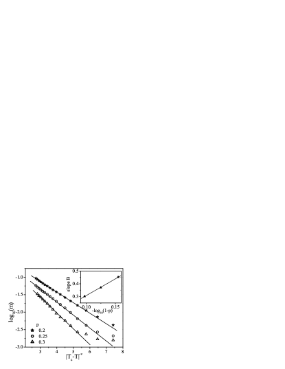
Figure 2: Logarithm of the total magnetization $m$ as a function of $|T_{c}^{0}-T|^{-\nu}$ ($\nu=0.627$) for several impurity concentrations $p=0.2,0.25,0.3$, averaged over 240 disorder realizations. System size $L_{\bot}=200$, $L_{C}=280$. The statistical errors are smaller than a symbol size for all $\log_{10}(m)>-2.5$. Inset: Decay slope $B$ as a function of $-\log(1-p)$.

The standard deviation of the total magnetization is below $10^{-3}$. For all three concentrations the data follow the analytical prediction, eq. (7), over more than an order of magnitude in $m$ with the exponent for the clean Ising model $\nu=0.627$. The deviation from the straight line for small $m$ is due to the conventional finite size effects (see discussion in subsection III.3). In the inset we show that the decay constant $B$ depends linearly on $-\log(1-p)$. This is the behavior expected from eq. (4).

III.3 Finite size effects and sample-to-sample fluctuations

As discussed in subsection II.3 one should distinguish between two different finite size effects, i.e., effects coming form the finite size $L_{C}$ in correlated direction and effects produced by the finite size $L_{\bot}$ in uncorrelated direction.

We start with analysis of the finite size effects in correlated directions, i.e. $L_{C}$ finite and $L_{\bot}\to\infty$. The true static order on the rare regions is destroyed by the finite length of the island in the correlated direction. For our model $d_{\perp}=1$ so no true static long range order can develop. The value of $m$ measured in the simulations is thus due to fluctuations which are governed by the central limit theorem, i.e., $m\sim V^{-1/2}$, where $V=L_{\bot}L_{C}^{2}$ is the volume of the system. This produces a conventional finite-size rounding responsible for the deviations of $m$ from the exponential law in Fig. 2. In Fig. 3, we investigate this finite-size effect in more detail.

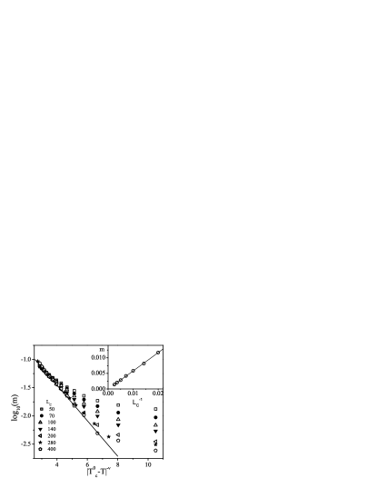
Figure 3: Logarithm of the total magnetization $m$ as a function of $|T_{c}^{0}-T|^{-\nu}$ ($\nu=0.627$) for disorder concentration $p=0.2$ and system sizes $L_{\bot}=200$, $L_{C}=50\ldots 400$. The statistical errors are smaller than about a symbol size. The solid line shows the analytic prediction, eq. (7). Inset: Total magnetization $m$ as a function of inverse length in the correlated direction $L_{C}$ for $T=4.5$ ($|T-T_{c}^{0}|^{-\nu}=16.91$).

This figure shows the total magnetization $m$ as a function of $|T_{c}^{0}-T|^{-\nu}$ for systems with fixed size in the uncorrelated direction $L_{\bot}=200$ and various lengths in the uncorrelated direction, $L_{C}=50,70,100,140,200,280,400$. The magnetization is averaged over 30 to 240 disorder realizations. As expected, for high temperatures, the total magnetization shows a strong dependence on $L_{C}$. The smallest systems follow the exponential behavior (7) only over a narrow range of temperatures and then cross over to the fluctuation determined value. If $L_{C}$ is increased the crossover between the exponential behavior (7) and the fluctuation background shifts to higher temperatures. In order to show that the fluctuation-determined value of the total magnetization $m$ at high temperatures indeed follows the predictions of the central limit theorem, i.e. $m\sim V^{-1/2}=(L_{\bot}L_{C}^{2})^{-1/2}\sim 1/L_{C}$ ($L_{\bot}$ is constant) we plot $m$ as a function of $1/L_{C}$ ($T=4.5$, $|T-T_{c}^{0}|^{-\nu}=16.91$). The numerical data shown in the inset of Fig. 3 can indeed be well fitted with a straight line. These results show that the small-$m$ deviations from the predicted behavior (7) are indeed the result of conventional finite-size rounding.

We now turn our attention to the more interesting finite size effects produced by the finite sample length $L_{\bot}$ in the uncorrelated direction. For sufficiently small $L_{\bot}$ one expects strong sample to sample fluctuations, as discussed in subsection II.3. In Fig. 4 we show the logarithm of the total magnetization $m$ as a function of $|T_{c}^{0}-T|^{-\nu}$ for three typical disorder realizations.

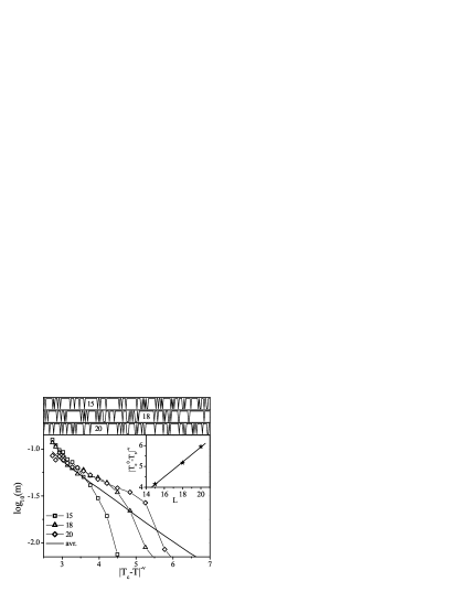
Figure 4: Logarithm of the total magnetization $m$ as a function of $|T_{c}^{0}-T|^{-\nu}$ for $L_{\bot}=200$, $L_{C}=280$ and $p=0.2$ for three different disorder realizations. The thermodynamic statistical error of $\log_{10}m$ of a single realization is about 0.1. Straight line represents the average over 240 disorder realizations. Upper panel: The coupling constant $J_{i}$ in the uncorrelated direction as a function of $i$ for the corresponding three disorder realizations. Numbers indicate length of the longest island $L_{i}$ in the uncorrelated direction. Inset: Relation between the sample critical temperature $T_{s}$ and the size of the island length, plotted as $|T_{c}^{0}-T_{s}|^{-\nu}$ as a function of island length.

For comparison, the upper panel of the Fig. 4 shows the coupling constant $J_{i}$ as a function of the position $i$ for the three samples. The numbers in the graph indicate the lengths of the longest islands $L_{i}$. The system size is $L_{\bot}=200$, $L_{C}=280$ with disorder concentration $p=0.2$. The solid line is the average magnetization over 240 disorder realizations. We see that all three curves qualitatively follow the average at low temperatures but start to deviate form it at higher temperatures. The temperature $T_{s}$ at which the magnetization of a sample rapidly drops is associated with the ordering of the largest island in this sample. Numerically, we determine $T_{s}$ as the temperature where the sample magnetizations falls below $1/3$ of the average magnetization. This definition contains some amount of arbitrariness which corresponds to an overall shift of all $T_{s}$. However, the leading functional dependence of $T_{s}$ on the size $L_{i}$ of the longest island in the sample is not influenced by this shift. In order to demonstrate this dependence we can apply finite size scaling for the clean $3d$ Ising model (islands are regions devoid of impurities) in the slab geometry, i.e. on a sample of length $L_{i}$ in one dimension and essentially infinite length in other two dimensions ($L_{C}\gg L_{i}$). In the inset of Fig. 4 we plot $|T_{c}^{0}-T_{s}|^{-\nu}$ as a function of $L_{i}$. The data show good agreement with the finite-size scaling prediction. Figure 4 also demonstrates that, in the tail of the smeared transition (for $T\to T_{c}^{0}$), the average (thermodynamic) magnetization is determined by rare samples with untypically large rare regions.

In Fig. 5, we show the probability distribution of the sample ordering temperature $T_{s}$ for system sizes $L_{\bot}=25,50,75,100,200$ and $L_{C}=200$, computed from 700 to 780 disorder realizations (the statistical error of the $T_{s}$ values is $\Delta T_{S}\lesssim 0.03$). The results are in good agreement with the predictions of subsection II.3, i.e., the probability distribution of the sample critical temperature becomes narrower and moves toward the clean critical temperature as the sample length $L_{\bot}$ in the uncorrelated direction is increased. In the inset of Fig. 5, we show that the width of the probability distribution (defined as its standard deviation) is proportional to $\log(L_{\bot})^{-1/\nu}$ as predicted in eq. (15).

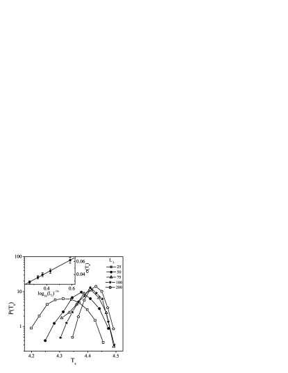
Figure 5: The probability distribution of sample critical temperature $T_{s}$ as for different sample lengths in the uncorrelated direction. The data shown is for system with $L_{\bot}=25,50,75,100,200$ and $L_{C}=200$. The probability distribution is calculated from 700 to 780 disorder realizations and disorder concentration $p=0.2$. Inset: Width of the probability distribution as a function of $\log(L_{\bot})^{-1/\nu}$.

III.4 Local magnetization

We now turn to the local (layer) magnetization $m_{i}$ (as for the total magnetization, our Monte-Carlo estimator is the average of the absolute values of the layer magnetizations for each measurement). Close to the clean critical point the system contains a few ordered islands (rare regions devoid of impurities) typically far apart in space. The remaining bulk system is essentially still in the disordered phase. Fig. 6 illustrates such a situation.

Figure 6: Local magnetization $m_{i}$ of a particular disorder realization as a function of the position $i$ in the uncorrelated direction (system size $L=200$, $L_{C}=200$ and temperature $T=4.425$). The statistical error is approximately $5\cdot 10^{-3}$. Lower panel: The coupling constant $J_{i}$ in the uncorrelated direction as a function of position $i$. Inset: Log-linear plot of the zoomed in region in the vicinity of the largest ordered island.

It displays the local magnetization $m_{i}$ of a particular disorder realization as a function of the position $i$ in the uncorrelated direction for the size $L_{\bot}=200$, $L_{C}=200$ at a temperature $T=4.425$ in the tail of the smeared transition. The lower panel shows the local coupling constant $J_{i}$ as a function of $i$. The figure shows that a sizable magnetization has developed on the longest island only (around position $i=160$). One can also observe that order starts to emerge on the next longest island located close to $i=25$. Far form these islands the system is still in its disordered phase. In the thermodynamic limit, the local magnetization should be exponentially small as predicted by eq. (10). However, in the simulations of a finite size system the local magnetization has a lower cut-off which is produced by finite-size fluctuations of the order parameter. These fluctuations are governed by the central limit theorem and can be estimated as $m_{bulk}\approx 1/\sqrt{N_{cor}}\approx\sqrt{L^{2}_{cl}/L^{2}_{C}}\approx 5\cdot 10^{-3}$ in agreement with the typical off-island value in Fig. 6. Here, $N_{cor}$ is the number of correlated volumes per slab as determined by the size off the Wolff cluster. $L_{cl}$ is a typical linear size of a Wolff cluster which is, at $T=4.425$, $L_{cl}\approx 10$). In the inset of Fig. 6 we zoom in on the region around the largest island. The local magnetization, plotted on the logarithmic scale, exhibits a rapid drop-off with the distance from the ordered island. This drop-off suggests a relatively small (a few lattice spacings) bulk correlation length $\xi_{0}$ in this parameter region.

As was discussed above, finite-size fluctuations of the local magnetization far form the ordered islands mask the true asymptotic behavior for very small $m_{i}$. In order to verify the probability distribution (13) of the local magnetization numerically, fluctuations have to be suppressed sufficiently. This would require simulating very large systems whose sizes in the correlated direction increase quadratically with the required magnetization resolution. With sizes available in our simulations we were not able to reproduce the distribution function, eq. (13), of $P(\log m_{i})$ predicted to be constant at small $m_{i}$ and calculated for the mean-field model.Vojta (2003b)

IV Conclusions

In this final section we summarize our results and discuss how the disorder induced smearing of the phase transition found here compares to the Griffiths phenomena. We also remark on favorable conditions for observing the disorder-induced smearing in experiments and simulations. Then we shortly discuss differences between models with discrete and continuous symmetry. We end by briefly addressing the question of smearing of quantum phase transitions.

We have performed large-scale Monte-Carlo simulations of a $3d$ Ising model with short-ranged, nearest neighbor interactions and planar defects, introduced via correlated bond disorder. The results of the simulations show that the phase transition is not sharp, but rather smeared over a range of temperatures by the presence of the extended defects. The numerical results are in good agreement with the theoretical predictions (see subsection II.2) based on the Lifshitz tail arguments.Vojta (2003a, b)

The physics behind the smearing of the phase transition discussed in this paper is similar to the physics underlying Griffiths phenomena. Both effects are produced by rare spatial regions which are devoid of impurities and therefore locally in the ordered phase while the bulk system is still disordered. The difference between Griffiths phenomena and disorder-induced smearing is a result of disorder correlations. If the disorder is uncorrelated or short-range correlated, the rare regions have finite size and cannot develop true static order. The order parameter on such a rage region still fluctuates, albeit slowly. These slow fluctuations lead to the well known Griffiths singularitiesGriffiths (1965) discussed in section I. In contrast, if the rare regions are infinite in two or more dimensions a stronger effect arises. The rare regions can develop true static long-range order independently of the rest of the system. The order parameter in such a system develops very inhomogeneously, which leads to the smearing of the phase transition. Therefore, exactly the same rare regions which would result in Griffiths phenomena if the disorder was short-range correlated lead to the smeared phase transition in the case of disorder correlated in two or more dimensions. In this sense the smearing of the transition takes the place of both the phase transition and the Griffiths region. Notice that long-range interactions increase the tendency toward smearing. If the interaction in the correlated direction falls off as $1/r^{2}$ or slower, even linear defects can lead to smearing, because a $1d$ Ising model with $1/r^{2}$ interaction has an ordered phase.Thouless (1969); Cardy (1981)

Now we turn our attention to favorable conditions for observing the smearing in numerical simulations or experiments. This turns out to be controlled by two conditions, one for the concentration of the impurities, and one for their strength. In order to easily observe the smearing, the concentration of rare regions, eq. (6), has to be sufficiently large. This requires a relatively small concentration of impurities. If the concentration of the impurities is too high, the exponential drop-off of the island number and thus of $m$ is very steep and the smearing effects would be very hard to observe. On the other hand, if the impurities are too weak, the smeared transition is too close to the clean critical point and the bulk critical fluctuations will effectively mask the smearing. Consequently, the best parameters for observing the smearing are a small concentration of strong impurities. This has been confirmed in test calculations using concentrations from $p=0.05$ to $0.5$. Unfavorable parameter values may also be the reason why no smearing has been observed in previous simulations.Lee and Gibbs (1992); Berche et al. (1998) Specifically, in Ref. Lee and Gibbs, 1992, simulations have been performed using a high concentration $p=0.5$ of weak impurities ($\Delta J/J=0.1$). The relatively small system sizes (up to $L=27$) in that simulation were probably not sufficient to observe the smearing.

The next remark concerns models with continuous order parameter symmetry. As pointed out above, the smearing of the phase transition is caused by static order on the rare regions. Thus, systems with continuous order parameter symmetry and short-range interactions would exhibit smearing of the phase transition only if the disorder is correlated in three or more dimensions.Mermin and Wagner (1966) Again, long-range interactions increase the tendency toward smearing. It is knownBruno (2001) that classical XY and Heisenberg systems in $1d$ and $2d$ develop long range order only if the interaction falls off more slowly than $1/r^{2d}$. Therefore a system with linear (planar) defects would show smearing of the phase transition if the interactions in the correlated direction would fall off more slowly then $1/r^{2}$ ($1/r^{4}$).

We end our discussion with the brief remark about smearing of quantum phase transitions in disordered itinerant electronic systems. Each quantum phase transition can be mapped to a classical phase transition in higher dimension, with imaginary time acting as additional dimension. For dirty itinerant ferromagnets the effective interaction between the spin fluctuations in the imaginary time direction falls off as $1/\tau^{2}$, and the disorder is correlated in this direction.Hertz (1976) Therefore, the dirty itinerant ferromagnetic transition is smeared even for point-like defects.Vojta (2003b)

In conclusion, we have presented results of Monte-Carlo simulations of a $3d$ Ising model with short-range interactions and planar defects. The numerical results show that the perfect disorder correlations in two dimensions destroy the sharp magnetic phase transition leading to a smeared transition at which the magnetization gradually develops over range of temperatures.