Formulation and Application of Quantum Monte Carlo Method to Fractional Quantum Hall Systems

Abstract

Quantum Monte Carlo method is applied to fractional quantum Hall systems. The use of the linear programming method enables us to avoid the negative-sign problem in the Quantum Monte Carlo calculations. The formulation of this method and the technique for avoiding the sign problem are described. Some numerical results on static physical quantities are also reported.

and

1 Introduction

Two-dimensional electron gas (2DEG) in a strong magnetic field is known as a system which shows various phenomena resulting from electronic interactions. In particular, the fractional quantum Hall (FQH) effect has attracted much theoretical and experimental attention as a correlation-dominated one peculiar to this system. To investigate such strongly correlated systems theoretically, numerical studies play a significant role. For example, the exact diagonalization and density matrix renormalization group (DMRG) methods [1] have been used for the study of FQH systems, because the ones are directly accessible to the ground state. However, the exact diagonalization can study static and dynamical properties only for small systems, while it is not so easy to obtain dynamical information by the DMRG calculations. Thus we apply the quantum Monte Carlo (QMC) method to this system in the present work.

The QMC method has been used for several quantum many-body systems. It can investigate both static and dynamical properties of systems larger than those to which the exact diagonalization is applicable. However, this method is inherently involved with the so-called negative-sign problem. Thus we need to overcome (at least, or moderate) the negative-sign nuisance in order to make the best use of the method. In this study, we formulate the QMC method to the FQH system that is free of the sign problem and report some numerical results.

2 General formalism of QMC at zero temperature

In the zero-temperature formalism, the expectation value of an observable $\mathcal{O}$ for a Hamiltonian $\mathcal{H}$ is given by

$$\langle\mathcal{O}\rangle=\lim_{\beta\to\infty}\langle\psi|e^{-\beta\mathcal{H}/2}\mathcal{O}e^{-\beta\mathcal{H}/2}|\psi\rangle/\langle\psi|e^{-\beta\mathcal{H}}|\psi\rangle,$$ (1)

where $|\psi\rangle$ is an arbitrary state not orthogonal to the ground state. Here we assume that the Hamiltonian can be written in a quadratic form of a one-body operator. When the imaginary-time evolution operator $e^{-\beta\mathcal{H}}$ is decomposed to imaginary-time slices $e^{-\Delta\beta\mathcal{H}}\cdots e^{-\Delta\beta\mathcal{H}}$, we perform the Hubbard-Stratonovich (HS) transformation for the quadratic form by introducing auxiliary fields for each time slice. Then the Hamiltonian is reduced to a linear form of the one-body operator and the expectation value is expressed in a form of an auxiliary-field path integral. We evaluate it by means of the Monte Carlo method. However, statistical weights used in this Monte Carlo calculation are not always positive for any auxiliary-field configuration and then the normalization denominator in Eq.(1) often becomes almost zero. Thus it is often impossible to calculate $\langle\mathcal{O}\rangle$ with sufficient precision. This disaster is called the negative-sign problem.

3 Hamiltonian

We consider interacting electrons confined on a spherical surface with a magnetic monopole located at the center of the sphere [2]. For simplicity, we neglect the spin degrees of freedom and assume that all the electrons occupy the lowest Landau level. Then single-particle states are specified by the $z$-component, $m$, of angular momentum whose amplitude is $s$, where $2s$ is the number of flux quanta piercing the sphere and $m$ ranges from $-s$ to $s$. The Hamiltonian can be written in a quadratic form of the density operator and its time reversal:

$${\mathcal{H}}=-\frac{1}{2}\sum_{K=0}^{2s}\chi_{K}\sum_{N=-K}^{K}\rho_{{}_{KN}}\tilde{\rho}_{{}_{KN}}+C_{0}\,\rho_{{}_{00}},$$ (2)

$$\rho_{{}_{KN}}\equiv\sum_{m_{1},m_{2}}\langle KN|m_{1}m_{2}\rangle(-1)^{s+m_{2}}\,a^{\dagger}_{m_{1}}a_{-m_{2}},~{}~{}~{}$$

where $a_{m}$ is an annihilation operator of electron, $\langle KN|m_{1}m_{2}\rangle$ the Clebsch-Gordan coefficient, and $C_{0}$ is a constant. The time reversal of the density operator is defined by $\tilde{\rho}_{{}_{KN}}=(-1)^{K}\,\rho^{\dagger}_{{}_{KN}}$. The coupling constant $\chi_{K}$ is related with the Haldane pseudopotential $V_{J}$ as

$$\chi_{K}=\sum_{J=0}^{2s}T_{KJ}V_{J},$$ (3)

$$T_{KJ}=(-1)^{2s-J+K+1}(2J+1)\begin{Bmatrix}s&s&J\\ s&s&K\end{Bmatrix},$$

where the braces denote Wigner’s $6j$ symbol. Since the transformation matrix $T$ satisfies $T^{-1}=T$, we also have a relation of

$$V_{J}=\sum_{K=0}^{2s}T_{JK}\chi_{K}.$$ (4)

The Hamiltonian in Eq.(2) can be written in a linear form of the density operator by the HS transformation. Denoting the auxiliary field for a mode $(KN)$ by $\sigma_{KN}$, the linearized Hamiltonian is given by

$$h(\sigma) = \sum_{K=1}^{2s}\eta_{K}\chi_{K}\left[\sum_{N=1}^{K}(\sigma_{KN}^{\ast}\rho_{KN}+\sigma_{KN}\tilde{\rho}_{KN})\right.$$

$$\left.+\frac{1}{2}(\sigma_{K0}^{\ast}\rho_{K0}+\sigma_{K0}\tilde{\rho}_{K0})\right]+\frac{1}{2}\chi_{0}\rho_{00}^{2}+C_{0}\rho_{00},$$

where $\eta_{K}=i$ when $\chi_{K}<0$ and $\eta_{K}=1$ for non-negative $\chi_{K}$. We note that $\rho_{00}$ is proportional to the number operator of electrons. Since the number of electrons is a conserved quantity in the zero-temperature formalism, the term $\chi_{0}\rho_{00}\tilde{\rho}_{00}$ and $C_{0}\,\rho_{{}_{00}}$ in Eq.(2) can be considered as constants.

4 Sign problem

In order to discuss the sign problem, we formulate here the auxiliary field path integral in a matrix representation. We first define the matrix elements of the linearized Hamiltonian by

$$-\Delta\beta\,h(\sigma)\,=\sum_{m,n=-s}^{s}M_{m,n}(\sigma)\,\alpha_{m}^{\dagger}\alpha_{n},$$ (5)

where

$$\alpha_{m}=\left\{\begin{array}[]{@{\,}ccl@{\,}}a_{m}&(m\geq 0),\\ (-1)^{s-m}a_{m}&(m<0).\end{array}\right.$$

Next, we represent the state $|\psi\rangle$ in Eq.(1) in terms of a matrix $V$ as

$$|\psi\rangle=(\sum_{m}\alpha_{m}^{\dagger}V_{{}_{m1}})(\sum_{m}\alpha_{m}^{\dagger}V_{{}_{m2}})\cdots(\sum_{m}\alpha_{m}^{\dagger}V_{{}_{mN_{e}}})|0\rangle,$$

where $N_{e}$ is the number of electrons. We remark that $M$ is a square matrix of dimension $2s+1$ and $V$ is a $(2s+1)\times N_{e}$ rectangular matrix. Then the denominator of the Eq.(1) is written as [3]

$$\langle\psi|e^{-\beta\mathcal{H}}|\psi\rangle=\int\mathcal{D}\sigma\,G(\sigma)\,\zeta(\sigma),$$

$$\mathcal{D}\sigma\equiv\prod_{i}\prod_{K=1}^{2s}\prod_{N=0}^{K}d^{2}\sigma_{KN}^{\left(i\right)},$$

$$G(\sigma) \equiv \prod_{i}\left\{\prod_{K=1}^{2s}\biggl{[}\frac{\Delta\beta|\chi_{K0}|}{4\pi}\prod_{N=1}^{K}\biggl{(}\frac{\Delta\beta|\chi_{KN}|}{2\pi}\biggl{)}\biggl{]}\right.$$

$$\times \left.\exp\biggl{[}-\Delta\beta\sum_{K=1}^{2s}|\chi_{K}|\biggl{(}\sum_{N=1}^{K}|\sigma_{KN}^{\left(i\right)}|^{2}+\frac{|\sigma_{K0}^{\left(i\right)}|^{2}}{2}\biggl{)}\biggl{]}\right\},$$

$$\zeta(\sigma) \equiv \langle\psi|e^{-\Delta\beta h(\sigma^{\left(N_{t}\right)})}\cdots e^{-\Delta\beta h(\sigma^{\left(2\right)})}e^{-\Delta\beta h(\sigma^{\left(1\right)})}|\psi\rangle$$ (6)

$$= \det\left[V^{\dagger}e^{M(\sigma^{(N_{t})})}\cdots e^{M(\sigma^{(2)})}e^{M(\sigma^{(1)})}V\right],$$

where $N_{t}=\beta/\Delta\beta$ is the number of the imaginary-time slices.

The sign problem is brought about by the fact that $\zeta(\sigma)$ can be negative. However $\zeta(\sigma)$ is forced to be non-negative under the following conditions [4]:
(i) $2s$ is odd and $N_{e}$ is even,
(ii) the coupling constants in the Hamiltonian satisfy $\chi_{K}\geq 0$ for $K=1,2,\cdots,2s$.
We show this as follows. From the condition (i), the indices, $m$ and $n$, of the matrix $M(\sigma)$ in Eq.(5) take the values, $\pm\frac{1}{2},\pm\frac{3}{2},\cdots,\pm s$. The matrix $M(\sigma)$ under the above conditions satisfies two relations as $M_{-m,-n}(\sigma)=M_{m,n}^{\ast}(\sigma)$ and $M_{-m,n}(\sigma)=-M_{m,-n}^{\ast}(\sigma)$ for positive $m$ and $n$. When the matrix $V$ satisfies $V_{-m,N_{e}/2+i}=V_{m,i}^{\ast}$ and $V_{-m,i}=-V_{m,N_{e}/2+i}^{\ast}$ for positive $m$ and $i=1,\cdots,N_{e}/2$, then the matrix in Eq.(6) can be written as

$$V^{\dagger}e^{M(\sigma^{(N_{t})})}\cdots e^{M(\sigma^{(1)})}V=\left[\begin{array}[]{@{\,}cc@{\,}}A&B\\ -B^{\ast}&A^{\ast}\end{array}\right],$$

where $A$ and $B$ are square matrices of dimension $N_{e}/2$. This type of matrix always has paired eigenvalues that are complex-conjugate each other. In fact, denoting a matrix of the above form and its eigenvalue by $X$ and $\lambda$, respectively, the complex conjugation of the proper equation yields the one on $\lambda^{\ast}$:

$$0 = \det\left[\left[\begin{array}[]{@{\,}cc@{\,}}{\bf 0}&-{\bf 1}\\ {\bf 1}&{\bf 0}\end{array}\right]X\left[\begin{array}[]{@{\,}cc@{\,}}{\bf 0}&{\bf 1}\\ -{\bf 1}&{\bf 0}\end{array}\right]-\lambda^{\ast}\right]=\det\left[X-\lambda^{\ast}\right].$$

That is, $\lambda^{\ast}$ is also an eigenvalue of $X$ and thus the determinant of this type of matrix is always non-negative, which leads to the desired condition that $\zeta(\sigma)\geq 0$.

Now we consider which FQH systems satisfy the above conditions. The condition (i) can be satisfied, for example, in case of $2s=3N_{e}-3$ for the $\nu=1/3$ Laughlin state [2], or $2s=2N_{e}-3$ for the Pfaffian state [5]. However, the condition (ii) is not satisfied when the values for the Coulomb interaction are used for $V_{J}$ in Eq.(3). Thus we need to control the value of $\chi_{K}$ (that is, that of $V_{J}$) by solving a linear programming problem in order to satisfy the condition (ii). Namely, taking into account that only $V_{J}$ for odd $2s-J$ are physical for fermionic systems, we inquire which set of $\chi_{K}$ minimizes

$$F(\chi_{0},\chi_{1},\cdots,\chi_{2s})\equiv\sum_{2s-J:{\rm odd}}\lambda_{J}(\sum_{K=0}^{2s}T_{JK}\chi_{K}-V_{J})$$ (8)

under the conditions: $\chi_{0}\leq 0$, $\chi_{K}\geq 0$ for $K=1,2,\cdots,2s$, and $\lambda_{J}(\sum_{K=0}^{2s}T_{JK}\chi_{K}-V_{J})\geq 0$ for odd $2s-J$. We note here that $\lambda_{J}$ controls the variance of pseudopotential from that for the Coulomb interaction for each $J$. In the present study we always set $\lambda_{J}=1$. Negative $\chi_{0}$ is needed to make $V_{0}$ ($=\sum_{K}T_{0K}\chi_{K}$) positive under the fact that $T_{0K}<0$ for all $K$. Thus obtained $\chi_{K}$ minimizes the variance from that for the Coulomb interaction satisfying the condition (ii).

5 Numerical results

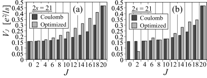
Figure 1 (a) shows an example of pseudopotentials free of the negative-sign problem. Although the optimized potentials do not coincide completely with those for the Coulomb interaction, their monotonical dependence on $J$ is realized naturally. We show another example of sign-problem free potential in Fig.1(b). To get the short-range components closer to those for the Coulomb potential, we bring long-range components close to zero. Namely, we set $V_{0}=V_{2}=0$ in Eq.(8). As a result, variance of short-range components from those of the Coulomb potential is squeezed. We note that optimized pseudopotentials can be obtained with less variance for higher Landau levels or in the presence of finite-thickness effects.

Figure 1: Pseudopotentials for the Coulomb interaction and negative-sign-free potentials obtained by the linear programming method for $2s=21$. The referred potential in the linear programming method is the Coulomb potential in (a), but in (b) long-range components, $V_{0}$ and $V_{2}$, of the referred potential are set to be zero. Only the physical ($2s-J$: odd) components are shown.

Figure 2: Expectation values of (a) energy per particle and (b) total angular momentum by the QMC calculation are shown versus inverse temperature for $2s=21$ and $N_{e}=8$. Optimized potential in Fig.1(b) was used. The values used as imaginary-time slice width are $\Delta\beta=1/8$, $1/16$, and $1/32$ in units of $1/(e^{2}/l_{B})$. The ground state energy obtained by the exact diagonalization is shown by an arrow on the right side of (a).

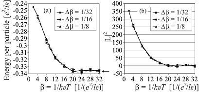
In Figure 2, we show expectation values of energy and total angular momentum against the inverse temperature $\beta$. Although finite value of $\Delta\beta$ gives rise to numerical errors in the Suzuki-Trotter decomposition, expectation values almost saturate for $\Delta\beta\leq 1/8\,(e^{2}/l_{B})$ ($l_{B}\equiv\sqrt{c/eB}$: the magnetic length). For comparison, we show the ground state energy obtained by the exact diagonalization by an arrow in Fig.2(a). It is noted that the total angular momentum of the true ground state is zero.

We find that for $\beta>20/(e^{2}/l_{B})$ these two quantities converge to the values expected for the ground state. In fact, the value of energy gap is about $0.1e^{2}/l_{B}$ in our exact diagonalization study, and thus the $\beta$-value choice of $\beta>20$ is appropriate to investigate the ground state properties. In case of smaller energy gap, larger values of $\beta$ are needed for the convergence of expectation values. Thus incompressible gapful states are more suitable than gapless ones for the study by the present method.

It is significant to discuss whether the ground state for negative-sign-free interaction is similar to that for the Coulomb interaction. Unfortunately the overlap between these two states for $\nu=1/3$ is not so large ($\sim 0.38$) for the pseudopotentials shown in Fig.1(b). Since the negative-sign-free interaction with $V_{2s-1}$ quite larger than $V_{2s-3}$ is expected to stabilize the Laughlin state as the lowest-energy state, the small overlap value seems to come from the reduction in long-range components. However, taking into account the fact that the ground state is gapful and the overlap is finite, the ground state for the negative-sign-free interaction is considered to capture essential properties of the Laughlin state.

6 Acknowledgement

One of the authors (S.S.) acknowledges support by Research Fellowship for young scientists of JSPS. The present work is supported by Grant-in-Aid for Scientific Research (Grant No.1406899 and No.14740181) by the Ministry of Education, Culture, Sports, Science and Technology of Japan.

References

- [1] D. Yoshioka, B.I. Halperin, and P.A. Lee, Phys. Rev. Lett. 50 (1983) 1395. N. Shibata and D. Yoshioka, ibid. 86 (2001) 5755.
- [2] F. D. M. Haldane, Phys. Rev. Lett. 51 (1983) 605.
- [3] E. Y. Loh Jr. and J. E. Gubernates, in Electronic Phase Transitions, edited by W. Hanke and Yu. V. Kopaev (Elsevier Science Publishers B. V., New York, 1992).
- [4] G. H. Lang, C. W. Johnson, S. E. Koonin, and W. E. Ormand, Phys. Rev. C 48 (1993) 1518.
- [5] G. Moore and N. Read, Nucl. Phys. B 360 (1991) 362.