Solitons in tunnel-coupled repulsive and attractive condensates

Abstract

We study solitons in the condensate trapped in a double-well potential with far-separated wells, when the $s$-wave scattering length has different signs in the two parts of the condensate. By employing the coupled-mode approximation it is shown that there are unusual stable bright solitons in the condensate, with the larger share of atoms being gathered in the repulsive part. Such unusual solitons derive their stability from the quantum tunneling and correspond to the strong coupling between the parts of the condensate. The ground state of the system, however, corresponds to weak coupling between the condensate parts, with the larger share of atoms being gathered in the attractive part of the condensate.

I Introduction

Bose-Einstein condensates (BECs) in trapped dilute gases exhibit interplay between quantum and nonlinear phenomena, since at zero temperature the mean-field Gross-Pitaevskii (GP) equation GPE for the order parameter applies with a good accuracy. The macroscopic quantum coherence of BEC was demonstrated experimentally intrfexp ; intrf2comp and explained theoretically intrfth with the use of the GP equation (see also the review Ref. BECRev ). One of the manifestations of nonlinear dynamics in BEC is appearance of solitons, i.e. the self-localized “waves of matter”, in quasi one-dimensional (cigar-shaped) condensates.

Nonlinear phenomena in BECs, and the solitons in particular, are similar to that in nonlinear optics, for instance, in optical fibers optfiber . In both fields the nonlinear Schrödinger (NLS) equation appears at some level of approximation. Similar to optics, where bright and dark solitons are supported respectively by the focusing and defocusing nonlinearities, in BECs the $s$-wave scattering length is the determining factor. Dark solitons are now routinely observed in the condensates with repulsive interactions dark1 ; dark2 ; dark3 ; dark4 , while the condensates with attractive interactions allow for stable bright solitons bright1 ; bright2 .

The similarity with optics, however, does not go so far as the control over nonlinearity in the governing equations. Atomic interactions in BEC can be tuned at one’s will by application of magnetic field near the Feshbach resonance fesh . This opens a possibility to observe new phenomena in BEC when the atoms interact differently in different spatial locations of the trap due to the presence of an external field. Though such a setup has not been yet realized experimentally, it cannot be rendered as impossible at the theoretical level. For BECs constrained to lower dimensions, the Feshbach resonance proves to be sharp due to many-body effects, for instance, it is so in the two-dimensional condensate Feshb2D . Similar result can be expected for the effectively one-dimensional BECs. The feasibility of control over the scattering length in BEC by the optical means is also being discussed optcontr (see also Refs. opt1 ; opt2 ).

Control over the scattering length in a part of the condensate can be realized in the double-well trap with far-separated wells, with the gradient of the external field being localized in the region of the barrier where the order parameter is exponentially small. For such setup the well-known two-mode approximation applies, which considerably simplifies the governing equations and allows for the analytical study. The asymmetric double-well potential is created by focusing an off-resonant intense laser beam near the center of a parabolic magnetic trap. Such setup is routinely realized in experiments (see, for instance, Ref. intrfexp ).

The goal of the present paper is to understand the nature of the unusual bright solitons in the condensate trapped in an asymmetric double-well potential, when the larger share of atoms is localized in the well where the atomic interactions are vanishing or weakly repulsive. Such counterintuitive solitons, due to the usual association of bright solitons with attractive interactions, were recently numerically discovered PhysD . However, the analytical form of the solitons and the domain of their existence were not addressed in the previous publication. In the present paper we analytically study the solitons and the domain of their existence.

Nonlinear phenomena in BEC in the double-well trap have already attracted a great deal of attention. The coherent atomic tunneling between the two wells and the macroscopic quantum self-trapping phenomenon were theoretically predicted in Refs. tunnel1 ; tunnel2 ; tunnellimit . In Ref. tunnellimit , the predictions of the mean field approach based on the GP equation were also compared with the results from the full quantum model. The conclusion is that the characteristic time scale on which the quantum collapse and revival dynamics starts to play a significant role is large and increases with the number of BEC atoms, while on the smaller time scale the GP equation gives a quantitatively accurate description. Similar conclusions were derived recently in Ref. smalltunnl . The general coupled-mode theory for the double-well trap with strong tunneling was developed in Ref. couplmod using the concepts of the nonlinear guided-wave optics. Nonlinear modes of the condensate in the double-well trap were used as the basis functions. Finally, the possibility of observing a chaotic dynamics of the condensate trapped in a double-well potential was the subject of Ref. chaotdyn . An effective amplitude equation was derived, which exhibited a behavior resembling that of the Lorentz system.

The paper is organized as follows. In the next section, complemented with the appendix, we give a self-consistent derivation of the coupled mode system for the asymmetric double-well trap with weak tunneling through the barrier. The general properties of the solitons in the coupled-mode system are summarized in section III.1. In section III.2, we derive an approximate analytical form of the soliton solutions in the case of vanishing interactions in one of the condensates. The exact boundary of the soliton bifurcation form zero, which defines the domain of existence of the stable solitons with the larger share of atoms in the repulsive condensate, is found in section III.3. Section IV contains discussion of the predicted phenomena. Finally, all numerical simulations in the present paper were performed with the use of the spectral collocation methods SP known for their high-accuracy. More details can be found in Ref. PhysD .

II Reduction of the GP equation to the coupled-mode system

Consider BEC trapped in an asymmetric double-well potential and assume that each of the wells is weakly confining in the $x$-direction and strongly confining in the transverse plane $\vec{r}_{\perp}\equiv(y,z)$. Let the transverse trap be parabolic in the $z$-direction and have the double-well shape in the $y$-direction, see fig. 1.

The zero-point energy difference between the two wells (shown by the dashed lines in fig. 1) can be managed, moving the position of the barrier-generating laser beam. We can neglect the small variation of the trap potential in the $x$-direction. The corresponding Gross-Pitaevskii (GP) equation for the order parameter $\Psi$ of the condensate then reads

$$i\hbar\frac{\partial\Psi}{\partial t}=\left\{-\frac{\hbar^{2}}{2m}\left(\frac{\partial^{2}}{\partial x^{2}}+\nabla_{\vec{r}{}_{\perp}}^{2}\right)+\mathcal{V}_{\mathrm{ext}}(\vec{r}_{\perp})+g|\Psi|^{2}\right\}\Psi,$$ (1)

with the external potential

$$\mathcal{V}_{\mathrm{ext}}=\frac{m\omega_{\perp}^{2}}{2}(y^{2}+\gamma^{2}z^{2})+\mathcal{V}_{B}\exp\left\{-\frac{(y-y_{0})^{2}}{2\sigma^{2}}\right\},\quad\mathcal{V}_{B}>0.$$ (2)

Here the parameter $\gamma$ accounts for the trap asymmetry in the transverse plane, while the parameters $y_{0}$ and $\sigma$ give the position and the width of the barrier, respectively.

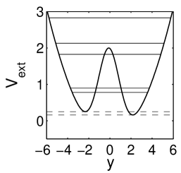
Figure 1: Illustration of the double-well: the parabolic trap potential in the $y$-direction modified by a Gaussian barrier. The (horizontal) solid lines indicate the numerically computed eigenvalues in the combined potential. The dashed lines show the bottom energies in the two wells of the trap. We use dimensionless units.

The double-well potential $\mathcal{V}_{\mathrm{ext}}$ is assumed to have two quasi-degenerate energy levels:

$$E_{1}-E_{0}\ll E_{2}-E_{1},$$ (3)

fig. 1 can serve as an illustration. There is a natural choice of the basis wave functions in the degenerate subspace, say $\psi_{u}$ and $\psi_{v}$, where each one is localized in just one of the wells. Such basis is given by a rotation of the wave functions for the ground and the first excited states:

$$\psi_{u}(\vec{r}_{\perp})=\frac{\psi_{0}(\vec{r}_{\perp})+\varkappa\psi_{1}(\vec{r}_{\perp})}{\sqrt{1+\varkappa^{2}}},\quad\psi_{v}(\vec{r}_{\perp})=\frac{\varkappa\psi_{0}(\vec{r}_{\perp})-\psi_{1}(\vec{r}_{\perp})}{\sqrt{1+\varkappa^{2}}}.$$ (4)

The choice of the parameter $\varkappa$ is based on the fact that the quotients of the absolute values of the eigenfunctions $\psi_{0}(\vec{r}_{\perp})$ and $\psi_{1}(\vec{r}_{\perp})$ at the extremal points $y_{-}$ and $y_{+}$ (in the two wells) are in approximate inverse proportionality relation

$$\frac{\psi_{1}(y_{-})}{\psi_{0}(y_{-})}\approx-\frac{\psi_{0}(y_{+})}{\psi_{1}(y_{+})}$$ (5)

(the positions of the extremals of the wave functions slightly deviate from each other and from the minima of the trap; these deviations we neglect). Equation (5) holds for the basis functions of the degenerate subspace for a general asymmetric double-well trap with weak tunneling through the barrier (see the appendix). For the double-well of fig. 1 the quotients of the eigenfunctions shown in fig. 2 have the values $3.1$ at the left and $-2.9$ at the right minima of the trap. We set $\varkappa={\psi_{1}(y_{-})}/{\psi_{0}(y_{-})}$. For this choice of $\varkappa$ the wave functions $\psi_{u}(y)$ and $\psi_{v}(y)$ defined by equation (4) are localized in the left and right wells, respectively, see fig. 2.

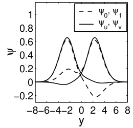
Figure 2: The ground and first excited state wave functions for the double-well trap in fig. 1 (dashed lines) and the wave functions localized in the complementary wells (solid lines) constructed as indicated in the text. All units are dimensionless.

For not too large number of atoms (see condition (10) below) one can neglect the higher excited levels of the trap and approximate the solution to the GP equation (1) as follows

$$\Psi(x,\vec{r}_{\perp},t)=f_{u}(x,t)\psi_{u}(\vec{r}_{\perp})+f_{v}(x,t)\psi_{v}(\vec{r}_{\perp}).$$ (6)

This approximation allows for reduction of the GP equation to a system of linearly coupled equations (equations (7) below) for the projections $f_{u,v}$ of the order parameter on the localized basis, due to approximate decoupling of the basis functions in the nonlinear term. For the double-well given in fig. 1, for instance, we obtain the following nonlinear cross-products:

$$\frac{\int\mathrm{d}y\psi_{u}^{2}\psi_{v}^{2}}{\int\mathrm{d}y\psi_{u}^{4}}=0.006,\quad\frac{\int\mathrm{d}y\psi_{u}\psi_{v}^{3}}{\int\mathrm{d}y\psi_{u}^{4}}=0.013,\quad\frac{\int\mathrm{d}y\psi_{u}^{3}\psi_{v}}{\int\mathrm{d}y\psi_{u}^{4}}=-0.040,\quad\frac{\int\mathrm{d}y\psi_{v}^{4}}{\int\mathrm{d}y\psi_{u}^{4}}=1.00.$$

Substituting expansion (6) into equation (1), multiplying by the localized wave functions, integrating over the transverse variables $y$ and $z$, and throwing away small nonlinear cross-terms we arrive at the coupled-mode system of Refs. tunnel1 ; tunnel2 but with the kinetic terms:

$$i\hbar\frac{\partial f_{u}}{\partial t}=-\frac{\hbar^{2}}{2m}\frac{\partial^{2}f_{u}}{\partial x^{2}}+(E_{u}+g_{u}|f_{u}|^{2})f_{u}-Kf_{v},$$ (7a)

$$i\hbar\frac{\partial f_{v}}{\partial t}=-\frac{\hbar^{2}}{2m}\frac{\partial^{2}f_{v}}{\partial x^{2}}+(E_{v}+g_{v}|f_{v}|^{2})f_{v}-Kf_{u}.$$ (7b)

The zero-point energies $E_{u}$ and $E_{v}$ and the tunneling coefficient $K$ are defined as follows:

$$E_{u,v}=\int\left(\frac{\hbar^{2}}{2m}(\nabla_{\vec{r}_{\perp}}\psi_{u,v})^{2}+\mathcal{V}_{\mathrm{ext}}(\vec{r}_{\perp})\psi_{u,v}^{2}\right)\mathrm{d}^{2}\vec{r}_{\perp},\quad g_{u,v}=\int g\psi_{u,v}^{4}\mathrm{d}^{2}\vec{r}_{\perp},$$ (8)

$$K=-\int\left(\frac{\hbar^{2}}{2m}(\nabla_{\vec{r}_{\perp}}\psi_{u})(\nabla_{\vec{r}_{\perp}}\psi_{v})+\psi_{u}\mathcal{V}_{\mathrm{ext}}(\vec{r}_{\perp})\psi_{v}\right)\mathrm{d}^{2}\vec{r}_{\perp},$$ (9)

here the $z$-dependence of the wave functions $\psi_{u}$ and $\psi_{v}$ is given by the ground state wave function (the Gaussian) in the $z$-direction (note that by changing the sign of either $\psi_{u}$ or $\psi_{v}$, if necessary, one can always set $K>0$). Below, we assume that the atomic interaction in the $v$-condensate is externally modified.

In the above analysis we have neglected the effect of nonlinearity on the dynamics in the transverse ($y,z$)-plane assuming a small contribution from the atomic interaction as compared to the energy gap $E_{2}-E_{1}$ of the trap. This leads to the following condition for each of the two parts of the condensate:

$$\frac{|a_{s}|\mathcal{N}}{\ell}\ll 1,$$ (10)

where $\mathcal{N}$ is the number of atoms, $a_{s}$ is the scattering length, and $\ell$ is the length of the condensate. Equation (10) is the usual condition of applicability of the one-dimensional NLS equation for the cigar-shaped condensate. The condition of applicability of the classical mean-field approach is $|a_{s}|/\ell\ll 1$ and $\mathcal{N}\gg 1$ (see, for instance, Ref QvsCc ), which is satisfied for large number of atoms and condition (10). Finally, the general applicability condition for our two-mode approximation reads $K\ll\hbar\omega_{\perp}$ (see the appendix).

In the calculations it is convenient to use a dimensionless form of system (7) with the following dimensionless variables:

$$\xi=\frac{x}{d_{\perp}},\quad d_{\perp}\equiv\left(\frac{\hbar}{m\omega_{\perp}}\right)^{1/2},\quad\tau=\frac{\omega_{\perp}}{2}t,\quad\varepsilon=\frac{2(E_{v}-E_{u})}{\hbar\omega_{\perp}},\quad\kappa=\frac{2K}{\hbar\omega_{\perp}},\quad a=\frac{a_{v}}{|a_{u}|}.$$ (11)

Here $a_{u}$ ($a_{u}<0$) and $a_{v}$ are defined as follows: $a_{u,v}\equiv d^{2}_{\perp}\int a_{s}\psi_{u,v}^{4}\mathrm{d}^{2}\vec{r}_{\perp}$ with $a_{s}$ being the $s$-wave scattering length (different in the two condensates). Introducing the dimensionless order parameters for the condensates in the two wells,

$$u(\xi,\tau)=e^{i\frac{E_{u}t}{\hbar}}(8\pi|a_{u}|)^{1/2}f_{u},\quad v(\xi,\tau)=e^{i\frac{E_{u}t}{\hbar}}(8\pi|a_{u}|)^{1/2}f_{v},$$ (12)

we arrive at the coupled-mode system suitable for the numerical study:

$$i\frac{\partial u}{\partial\tau}+\frac{\partial^{2}u}{\partial\xi^{2}}+|u|^{2}u+\kappa v=0,$$ (13a)

$$i\frac{\partial v}{\partial\tau}+\frac{\partial^{2}v}{\partial\xi^{2}}-(\varepsilon+a|v|^{2})v+\kappa u=0.$$ (13b)

The number of particles in the coupled-mode system (13), defined as $N_{u}=\int\mathrm{d}\xi|u|^{2}$ and $N_{v}=\int\mathrm{d}\xi|v|^{2}$, is related to the actual number of atoms $\mathcal{N}$ as follows: $\mathcal{N}_{u,v}=(d_{\perp}/8\pi|a_{u}|)N_{u,v}$ (the coefficient $d_{\perp}/8\pi|a_{u}|$ is of order $10^{2}-10^{3}$). Note that the quotient of the number of atoms in the two condensates does not change under the scaling transformation. Below we will use only the quantity $N_{u,v}$ referring to it as “the number of atoms” for simplicity.

Finally, we note an important difference between our approach and that of Ref. couplmod . In the latter work the nonlinear modes are used as the basis functions, what results in an effective coupled-mode system with nonlinear cross-terms, whereas our system (13) consists of linearly coupled equations. Our coupled-mode system, however, applies only in the case of weak tunneling through the barrier. But precisely in such setup the experimental realization of control over the scattering length in a part of the condensate may be feasible.

III Solitons in the tunnel-coupled condensates

III.1 General properties of the soliton solutions to the coupled-mode system

We are interested in the stable stationary soliton solutions to the coupled-mode system (13) mainly for $a\geq 0$, i.e. for a repulsive-attractive pair of condensates. Setting $u=e^{-i\mu\tau}U(\xi)$ and $v=e^{-i\mu\tau}V(\xi)$, where $\mu$ is the dimensionless chemical potential and the functions $U(\xi)$ and $V(\xi)$ are real, we obtain the corresponding stationary system for the soliton profiles:

$$\mu U+U_{\xi\xi}+U^{3}+\kappa V=0,$$ (14a)

$$(\mu-\varepsilon)V+V_{\xi\xi}-aV^{3}+\kappa U=0.$$ (14b)

The two-mode approximation requires that $\kappa\ll 1$ and $|\varepsilon|\ll 1$. On the other hand, system (14) admits the following scaling invariance:

$$U=\sqrt{\kappa}\,\tilde{U},\quad V=\sqrt{\kappa}\,\tilde{V},\quad\xi=\frac{\tilde{\xi}}{\sqrt{\kappa}},\quad\mu=\kappa\tilde{\mu},\quad\varepsilon=\kappa\tilde{\varepsilon},$$ (15)

where the new variables with tilde satisfy the same system with $\tilde{\kappa}=1$. For this reason we will keep $\varepsilon$ and $\kappa$ arbitrary. The scale-invariance (15) can be used to verify the analytical solutions.

We are interested in the so-called fundamental solitons, i.e. when the functions $U(\xi)$ and $V(\xi)$ are nodeless and decreasing exponentially as $|\xi|\to\infty$. The exponential decay rate $k$, $U\sim e^{-k\xi}$ and $V\sim e^{-k\xi}$ as $\xi\to\infty$, is given by the dispersion law of the linearized system. One obtains the following two branches:

$$k_{1,2}=\sqrt{\mu_{1,2}-\mu},\quad\mu_{1}=\frac{\varepsilon}{2}-\sqrt{\frac{\varepsilon^{2}}{4}+\kappa^{2}},\quad\mu_{2}=\frac{\varepsilon}{2}+\sqrt{\frac{\varepsilon^{2}}{4}+\kappa^{2}}.$$ (16)

Note that for arbitrary $\kappa$ and $\varepsilon$ the boundary chemical potentials satisfy the inequality $\mu_{1}<0<\mu_{2}$. They coincide with the two quasi-degenerate energy levels of the coupled-mode system (13) when the nonlinearities are negligible.

For $a\geq 0$ it can be shown that the two dispersion laws correspond to two possible classes of the fundamental soliton solutions: $UV>0$ or $UV<0$, below called the in-phase and out-phase solitons respectively. Indeed, the amplitudes $U_{0}\equiv U(0)$ and $V_{0}\equiv V(0)$ are bounded as follows PhysD :

$$U_{0}^{2}<-2\mu,\quad\mathrm{if}\quad UV>0;\qquad aV_{0}^{2}<2(\mu-\varepsilon),\quad\mathrm{if}\quad UV<0.$$ (17)

Noticing that the conditions $k_{1}^{2}>0$ and $k_{2}^{2}>0$ demand respectively $\mu<\mathrm{min}(0,\varepsilon)$ and $\mu>\mathrm{max}(0,\varepsilon)$ we see that the in-phase solitons correspond to the $k_{1}$-branch, while the out-phase ones pertain to the $k_{2}$-branch. Numerical calculations confirm this prediction PhysD .

We will discard the out-phase soliton solutions from consideration, since they bifurcate from zero at a higher chemical potential $\mu_{2}$ (16). Therefore, it is clear that they can be stable only in exceptional cases (they do not satisfy stability criterion (21) given below, consult also Ref. A2 ). Below by the soliton solution we will mean the in-phase soliton.

When the condensates are attractive, i.e. for $a<0$, there is a class of the sech-type soliton solutions PhysD , which generalizes the well-known symmetric solitons in the standard model of the dual-core optical fiber A2 ; A1 (see also the review Ref. ProgOpt ). The sech-type soliton solution is given as

$$\left(\begin{array}[]{c}U\\ V\end{array}\right)=\left(\begin{array}[]{c}A_{\mathrm{in}}\\ (-a)^{-1/2}A_{\mathrm{in}}\end{array}\right)\mathrm{sech}\left(\frac{A_{\mathrm{in}}\xi}{\sqrt{2}}\right),\quad A_{\mathrm{in}}=\sqrt{2\kappa}\left(-\mu/\kappa-(-a)^{-1/2}\right)^{1/2}.$$ (18)

It exists in the special case, when $\varepsilon$, $\kappa$, $a$, and $\mu$ are related as follows:

$$\varepsilon=\kappa\left[(-a)^{1/2}-(-a)^{-1/2}\right]\equiv h(\kappa,a),\quad\mu<\mu_{1}=-\kappa(-a)^{-1/2}.$$ (19)

Evidently, the exact sech-type soliton solution does not exist for $a\geq 0$.

There is another branch of the in-phase solitons, not known analytically, which bifurcates from the sech-type soliton branch (18), in the domain of their existence, at the point

$$\mu_{\mathrm{bif}}=-\kappa\,\frac{4-a}{3\sqrt{-a}},\quad\varepsilon=h(\kappa,a).$$ (20)

For other parameter values the sech-type solitons (18) and the bifurcating in-phase solitons coexist on separate curves $N=N(\mu)$ PhysD (here $N$ is the total number of atoms in the condensate). At least one of the two soliton branches must have continuation for positive values of $a$, since we have found such in-phase solitons numerically in Ref. PhysD (we have found exactly one branch for $a\geq 0$).

It is important to know the stability properties of the soliton solutions. In Ref. PhysD we have shown that for $a\geq 0$ the Vakhitov-Kolokolov criterion for the soliton stability

$$\frac{\partial N}{\partial\mu}<0$$ (21)

can be applied (consult also Refs. VK ; Zakh ). The stability property of the in-phase solitons for $a<0$ is affected by bifurcations (i.e. criterion (21) does not apply for all $\mu$ when $a<0$). Details can be found in Ref. PhysD .

III.2 Analytical soliton solutions for $a=0$

For $a=0$ the self-bound states, solitons, are possible due to the balance between the cubic nonlinearity in the attractive condensate and the linear dispersion in both condensates. Thus we can use the following strategy to find an approximate expression for the solitons. Equation (14b), which can be cast as

$$\Lambda V\equiv\left(1-\beta\frac{\mathrm{d^{2}}}{\mathrm{d}\xi^{2}}\right)V=\kappa\beta U-a\beta V^{3},\quad\beta\equiv(\varepsilon-\mu)^{-1},$$ (22)

can be explicitly resolved with respect to $V$ for $a=0$ using the method of the Green function. It was already mentioned that for the in-phase solitons $\mu<\varepsilon$ and hence $\beta>0$. Thus the operator $\Lambda$ is positive definite and invertible and the unique Green function reads $G(\xi)=\exp\{-|\xi|/\sqrt{\beta}\}/(2\sqrt{\beta})$. Therefore the solution to equation (22) for $a=0$ is

$$V(\xi)=\frac{\kappa\sqrt{\beta}}{2}\int\limits_{-\infty}^{\infty}e^{-\frac{|\xi-\eta|}{\sqrt{\beta}}}U(\eta)\mathrm{d}\eta.$$ (23)

Solution (23) can be expanded in the infinite series with respect to the derivatives of $U(\xi)$:

$$V(\xi)=\kappa\beta\left(U(\xi)+\sum_{n=1}^{\infty}\beta^{n}U^{(2n)}(\xi)\right),$$ (24)

which can be most easily verified by the formal inversion of the operator $\Lambda$. The crucial step in the derivation of the approximate soliton solution consists in retaining only two terms from the series (24) when it is substituted into the equation for $U(\xi)$, equation (14a). For such a reduction the following condition must be satisfied

$$U^{3}\gg\kappa^{2}\beta^{n+1}U^{(2n)},\quad n\geq 2.$$ (25)

Thus, under condition (25), the coupled-mode system (14) reduces to the canonical NLS

$$(\mu+\kappa^{2}\beta)U+(1+\kappa^{2}\beta^{2})U_{\xi\xi}+U^{3}=0.$$ (26)

In this approximation the $u$-component of the solution is given by the sech-type soliton:

$$U=A\mathrm{sech}(k\xi),\quad A\equiv\left[\frac{2(\mu_{1}-\mu)(\mu_{2}-\mu)}{\varepsilon-\mu}\right]^{1/2},\quad k\equiv\left[\frac{(\varepsilon-\mu)(\mu_{1}-\mu)(\mu_{2}-\mu)}{(\varepsilon-\mu)^{2}+\kappa^{2}}\right]^{1/2}.$$ (27)

Using the identities $\mu_{1}\mu_{2}=-\kappa^{2}$ and $\varepsilon=\mu_{1}+\mu_{2}$ it is easy to check that the amplitude $A$ satisfies the first inequality in equation (17) for all values of $\mu$. However, the analytical decay rate $k$ is not the same as $k_{1}$ in equation (16). This is the price we pay for adopting the approximation. In fact, as either $\mu\to\mu_{1}$ or $|\mu|\gg|\mu_{1}|$ (recall that $\mu<\mu_{1}<0$) the decay rate $k$ approaches $k_{1}$:

$$k=k_{1}\left[1+\mathcal{O}(\mu_{1}-\mu)\right],\quad k=k_{1}\left[1+\mathcal{O}(\mu_{1}/\mu)\right].$$ (28)

The applicability condition for the analytical approximation is then satisfied at least in these two limits. Indeed, condition (25) demands that $A^{3}\gg\kappa^{2}\beta^{3}k^{4}A$, where we have estimated $U_{\xi}\sim kU$, and after a simple transformation we obtain

$$\alpha^{2}\equiv\frac{(\mu_{1}-\mu)(\mu_{2}-\mu)}{(\varepsilon-\mu)^{2}+\kappa^{2}}\ll 1+\frac{(\varepsilon-\mu)^{2}}{\kappa^{2}}.$$ (29)

Moreover, comparison with the numerical solution shows that the analytical approximation captures all essential features of the number of atoms as function of the chemical potential for all values of $\mu$ (see fig. 3 below).

The $v$-component of the soliton, given by equation (23), cannot be found in the explicit form. Nevertheless, all the necessary physical quantities, for instance, the number of atoms $N_{v}(\mu)$ and the energy of the soliton, can be found in closed form. The shares $N_{u}$ and $N_{v}$ of the BEC atoms trapped in the two wells read:

$$N_{u}=4\left(\frac{(\mu_{1}-\mu)(\mu_{2}-\mu)[(\varepsilon-\mu)^{2}+\kappa^{2}]}{(\varepsilon-\mu)^{3}}\right)^{1/2},$$ (30)

$$N_{v}=4\kappa^{2}\frac{(\mu_{1}-\mu)(\mu_{2}-\mu)}{(\varepsilon-\mu)^{7/2}}\sum_{n=0}^{\infty}\frac{(2n+1)\alpha+3}{[(2n+1)\alpha+1]^{3}},$$ (31)

where $\alpha$ is defined in equation (29).

The deformation of the curves $N_{u}(\mu)$ and $N_{v}(\mu)$ given by equations (30) and (31) with variation of the zero-point energy difference $\varepsilon$ is illustrated in fig. 3 (we remind that the scaled number of atoms $N=(8\pi|a_{u}|/d_{\perp})\mathcal{N}$ is used). The qualitative behavior of the analytical curves is in excellent agreement with the numerical results of Ref. PhysD (the local maxima of the analytical curves $N_{u,v}(\mu)$ are narrower and 10% higher than the maxima of the numerical curves).

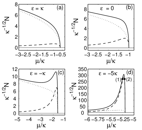
Figure 3: Behavior of the number of atoms in the two wells of the trap vs. the chemical potential with variation of the zero-point energy difference between the wells (all quantities pertain to the dimensionless system (13)). Here the dotted lines correspond to $N_{u}$, the dashed lines to $N_{v}$, and the solid ones to the total number of atoms $N=N_{u}+N_{v}$. In panel (d) only the part of the picture about the local maximum is shown (the full picture is similar to that in panel (c)).

Note the striking sensitivity of the total number of atoms and that of the fraction $N_{v}/N_{u}$ at the local maximum with respect to variation of the zero-point energy difference $\varepsilon$. From figs. 3(c) and (d) it is seen that a small variation of $\varepsilon$ (with $\varepsilon$ being on the order of a small tunneling coefficient $\kappa$) results in a large variation of both the total number of atoms and the relative share of atoms in the $v$-condensate.

The solitons corresponding to the two stars in fig. 3(d) are shown in fig. 4. Soliton-(1) is unstable while soliton-(2) is stable. The latter one represents the unusual self-bound state of the system, where almost all atoms are gathered in the noninteracting condensate.

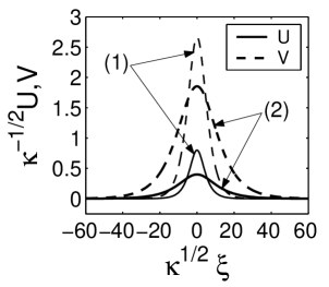
Figure 4: Unstable (1) and stable (2) soliton solutions to the dimensionless system (13) with the same total number of atoms which correspond to the two stars in panel (d) of fig. 3.

From fig. 3 it is seen that the soliton solution bifurcates from the zero solution at $\mu=\mu_{1}$. In fact, for $a=0$, the total number of atoms is indeed always equal to zero on the boundary of the soliton existence. For $\mu\to\mu_{1}$ the sum on the r.h.s. of equation (31) can be approximated as follows

$$\sum_{n=0}^{\infty}\frac{(2n+1)\alpha+3}{[(2n+1)\alpha+1]^{3}}=\sqrt{\mu_{2}}(\mu_{1}-\mu)^{-1/2}+\mathcal{O}\{(\mu_{1}-\mu)^{1/2}\},$$ (32)

where have used the Euler-Maclaurin summation formula and the definition of $\alpha$ (29). Hence, the number of atoms is proportional to $(\mu_{1}-\mu)^{1/2}$ as $\mu\to\mu_{1}$ and the bifurcation is continuous for $a=0$ (in contrast, the number of atoms has a finite limit as $\mu\to\mu_{1}$ for $a>0$ and $\varepsilon=\varepsilon_{\mathrm{cr}}$, see the next section).

From equations (30)-(32) one may deduce the ratio of the slopes of $N_{u}(\mu)$ and $N_{v}(\mu)$ as $\mu\to\mu_{1}$:

$$\lim_{\mu\to\mu_{1}}\frac{N_{v}}{N_{u}}=\frac{|\mu_{1}|}{\mu_{2}}=\frac{\sqrt{(\varepsilon/2)^{2}+\kappa^{2}}-\varepsilon/2}{\sqrt{(\varepsilon/2)^{2}+\kappa^{2}}+\varepsilon/2}.$$ (33)

This is the quantitatively accurate result, since in this limit condition (29) is well satisfied. Formula (33) predicts, for instance, that almost all atoms are gathered in the non-interacting condensate for $|\,\varepsilon|\gg\kappa$ and $\varepsilon<0$. Thus, to observe such unusual solitons the zero-point energy difference $\varepsilon$ should be decreased sufficiently below zero. Physically, it is clear that the energy decrease due to the attractive interaction in the $u$-condensate with increase of $N_{u}$ should be compensated by a lower zero-point energy in the $v$-well, if one wants to increase the ratio $N_{v}/N_{u}$.

Condition (29) breaks down about the local maximum of the curve $N=N(\mu)$ (see fig. 3(d)) and one has to use the whole infinite series expansion (24) for quantitatively correct description of the soliton in the system. Therefore, the condensates are strongly coupled when almost all atoms are trapped in the $v$-well. We will see below that the unusual solitons also appear for $0<a\ll 1$ and $\varepsilon_{\mathrm{cr}}<\varepsilon<0$, with almost all atoms being contained in the repulsive condensate strongly coupled by the quantum tunneling to the attractive one.

For $|\mu|\gg|\mu_{1}|$ we obtain the following estimates for the number of atoms in the two wells:

$$N_{u}=4\sqrt{-\mu}+\mathcal{O}(|\mu|^{-5/2}),\quad\frac{N_{v}}{N_{u}}=0.712\frac{\kappa^{2}}{\mu^{2}}+\mathcal{O}\left(\mu^{-3}\right),$$ (34)

where we have used $\alpha=1$ to evaluate the infinite sum in equation (31) (since $\alpha=1+\mathcal{O}(\mu^{-1})$). First of all, almost all atoms are gathered in the attractive $u$-condensate. Second, in this limit the $u$-component of the soliton solution asymptotically satisfies equation (14a) for $\kappa=0$, since the amplitude and decay rate of soliton (27) asymptotically approach those for the soliton solution of a single NLS equation: $A=\sqrt{-2\mu}+\mathcal{O}(|\mu|^{-3/2})$ and $k=\sqrt{-\mu}+\mathcal{O}(|\mu|^{-3/2})$. Thus, for large negative $\mu$ the coupled-mode system predicts weak coupling between the two condensates.

To determine the ground state of the system let us find the energy of the soliton solutions. The GP equation (1) corresponds to the energy functional

$$\mathcal{E}=\int\mathrm{d}^{3}\vec{r}\left\{\frac{\hbar^{2}}{2m}|\nabla\Psi|^{2}+\mathcal{V}_{\mathrm{ext}}|\Psi|^{2}+\frac{g}{2}|\Psi|^{4}\right\}.$$ (35)

In the coupled-mode approximation we have the following expression for the energy

$$\mathcal{E}=E_{u}\mathcal{N}+\frac{\hbar\omega_{\perp}d_{\perp}}{16\pi|a_{u}|}H,$$ (36)

where $\mathcal{N}$ is the actual total number of atoms and $H$ is the Hamiltonian for system (13):

$$H=\int\mathrm{d}\xi\left\{\left|\frac{\partial u}{\partial\xi}\right|^{2}+\left|\frac{\partial v}{\partial\xi}\right|^{2}+\varepsilon|v|^{2}-\kappa(uv^{*}+vu^{*})-\frac{|u|^{4}}{2}+\frac{a|v|^{4}}{2}\right\}.$$ (37)

The Hamiltonian $H$ evaluated on the soliton solution reads

$$H_{\mathrm{sol}}=-\frac{4}{3}\left[\frac{(\mu_{1}-\mu)^{3}(\mu_{2}-\mu)^{3}}{(\varepsilon-\mu)^{2}+\kappa^{2}}\right]^{1/2}\frac{(\varepsilon-\mu)^{2}+2\kappa^{2}}{(\varepsilon-\mu)^{5/2}}-4\kappa^{2}\frac{(\mu_{1}-\mu)(\mu_{2}-\mu)(2\varepsilon-3\mu)}{(\varepsilon-\mu)^{7/2}}S(\mu)$$ (38)

where $S(\mu)=\sum_{n=0}^{\infty}\frac{(2n+1)\alpha+\sigma}{[(2n+1)\alpha+1]^{3}}$ and $\sigma=\frac{2\varepsilon-5\mu}{2\varepsilon-3\mu}$. Taking into account that $2\varepsilon>\mathrm{max}(3\mu,5\mu$), since $\mu<\mu_{1}$, it is easy to see that $H_{\mathrm{sol}}$ is always negative. In the coupled-mode approximation, expression (38) is quantitatively correct for $\mu\to\mu_{1}$ and $|\mu|\gg|\mu_{1}|$, and for other values of $\mu$ captures the qualitative behavior of the energy. Note that $H$ scales as $\kappa^{3/2}$.

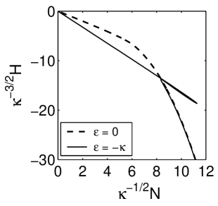
Figure 5: The energy vs. the total number of atoms (for the dimensionless system (13)) for two values of the zero-point energy difference: $\varepsilon=0$ (the dashed line) and $\varepsilon=-\kappa$ (the solid line). The solid line has a very narrow twist without self-intersection, which occupies the interval $8<N/\sqrt{\kappa}<12$.

Lowering $\varepsilon$ below zero forces the energy to develop a twist, see fig. 5. The twisted part of the curve widens by decreasing $\varepsilon$, while its left endpoint moves towards $N=0$. (The curve $H=H(N)$ has the shape similar to that of $\mu=\mu(N)$ after the following substitution is applied to the latter: $(\mu_{1}-\mu)\to-H$.) It follows that, for almost all values of $\varepsilon$ and the total number of atoms, the energy is minimized on the solutions with large negative $\mu$ (in fig. 5 the latter solitons correspond to the lower part of the solid line below the twist, while the unusual solitons pertain to the twisted part). However, according to criterion (21) the solitons with the larger share of atoms in the $v$-condensate are stable (precisely, the solitons which pertain to the upper part of the twist in fig. 5), thus they can be experimentally observed.

Finally, let us check condition (10). Estimating the condensate length as $\ell/d_{\perp}\sim k$, we get that in the dimensionless variables the one-dimensionality condition for the $u$-condensate is $kN_{u}\ll 1$. Using the explicit expressions (27) and (30) we arrive at $(\mu_{1}-\mu)(\mu_{2}-\mu)\ll\varepsilon-\mu$ which is satisfied for $\mu$ close to $\mu_{1}$, i.e. in the domain of the unusual solitons. Similar, for the $v$-condensate we have $k|a|N_{v}\ll 1$, which is satisfied for small $a$ in the same range of $\mu$. On the other hand, the soliton solutions with large negative $\mu$ may violate the one-dimensionality condition (it is violated in the limit $|\mu|\gg|\mu_{1}|$). It is a reflection of the fact that for large enough number of atoms the transverse degrees of freedom start to play a significant role for the weakly coupled condensates, i.e. for the ground state in the system, leading to the collapse instability at some $kN=f(k)$ (for details on collapse consult Ref. collapse ). However, for the number of atoms below the collapse instability threshold the ground-state soliton of the coupled-mode system is stable (but may have a modified shape), while the unusual solitons are effectively one-dimensional, since they always satisfy condition (10).

III.3 Solitons for $a>0$ and the boundary of the bifurcation from zero

We have seen that for $a=0$ the soliton solutions bifurcate from the zero solution at $\mu=\mu_{1}$ and the unusual stable solitons appear close to the bifurcation boundary. For $a>0$ the competition between the zero-point energy difference $\varepsilon$ and repulsion in the $v$-condensate creates a lower boundary $\varepsilon_{\mathrm{cr}}=b(k,a)$ for the bifurcation from zero. Thus for $a>0$ the unusual solitons appear only for $\varepsilon>\varepsilon_{\mathrm{cr}}$. Existence of such a boundary was discovered numerically in Ref. PhysD for $a=1$.

It turns out that $\varepsilon_{\mathrm{cr}}(k,a)$ can be found analytically in the exact form. To this goal we suppose that the solitons do bifurcate from zero and find the value of $\varepsilon$ for which we have a contradiction. Setting $\epsilon=\mu_{1}-\mu$, we assume that $U=\mathcal{O}(\epsilon^{p})$ and $V=\mathcal{O}(\epsilon^{q})$ as $\epsilon\to 0$, for some $p,q>0$. Using the estimate ${\mathrm{d}^{2}}/{\mathrm{d}\xi^{2}}\sim k^{2}_{1}=\epsilon$ and $\beta=(\mu_{2}+\epsilon)^{-1}=\mathcal{O}(1)$ in equation (22) we immediately obtain $q=p$. Note that the terms containing $U$ in equation (14a) have the following powers of $\epsilon$: $\mu U=\mathcal{O}(\epsilon^{p})$, $U_{\xi\xi}=\mathcal{O}(\epsilon^{p+1})$, and $U^{3}=\mathcal{O}(\epsilon^{3p})$, where we have used the above estimate for the second derivative. Therefore, irrespectively of the value of $p$, it is clear that if an expression for $V$ contains all the terms with powers of $\epsilon$ up to $\mathrm{max}(p+1,3p)$, it then contains all the necessary terms we need to derive the soliton solution in the lowest order of $\epsilon$.

The most general expression for $V$ that explicitly contains all the powers of $\epsilon$ up to $\mathrm{max}(p+1,3p)$ is as follows

$$V=F(U)+CU_{\xi\xi}+\mathcal{O}(\epsilon^{s}),\quad s\equiv\mathrm{min}(3p+1,p+2),$$ (39)

where the function $F(U)$ and the constant $C$ (of order 1) are determined by solution of equation (22) in the required order of $\epsilon$. We will need the expression for $V$ up to the terms of order $\epsilon^{5p}$ only. We obtain

$$V=\kappa\beta U-a\kappa^{3}\beta^{4}U^{3}+3a^{2}\kappa^{5}\beta^{7}U^{5}+\kappa\beta^{2}U_{\xi\xi}+\mathcal{O}(\epsilon^{r}),\quad r\equiv\mathrm{min}(3p+1,p+2,7p).$$ (40)

Here the coefficient $\beta=(\mu_{2}+\epsilon)^{-1}$ also should be expanded into powers of $\epsilon$.

Substitution of expression (40) into equation (14a) leads to the following equation for the $u$-component of the soliton:

$$-\epsilon\left(1-\frac{\mu_{1}}{\mu_{2}}\right)U+\left(1-\frac{\mu_{1}}{\mu_{2}}\right)U_{\xi\xi}+\left(1-\frac{a\kappa^{4}}{\mu_{2}^{4}}\right)U^{3}+\frac{3a^{2}\kappa^{6}}{\mu_{2}^{7}}U^{5}=\mathcal{O}(\epsilon^{r}).$$ (41)

From equation (41) it is quite clear that the bifurcation from zero is forbidden if the coefficient at the cubic nonlinear term is negative (we remind that $\mu_{2}>\mu_{1}$), i.e. if the lowest-order nonlinearity is repulsive. In the latter case equation (41) does not contain bright soliton solutions in the limit $\epsilon\to 0$. Hence, the exact boundary of the bifurcation from zero is given as $\mu_{2}(\varepsilon_{\mathrm{cr}},\kappa)=\kappa a^{1/4}$. Using the definition of $\mu_{2}$ (16), we obtain the critical value of the zero-point energy difference

$$\varepsilon_{\mathrm{cr}}=\kappa\left(a^{1/4}-a^{-1/4}\right).$$ (42)

There are no in-phase solitons bifurcating from the zero solution below the boundary $\varepsilon_{\mathrm{cr}}$.

The properties of solitons close to the bifurcation boundary $\mu_{1}$ are different in the two cases $\varepsilon>\varepsilon_{\mathrm{cr}}$ and $\varepsilon=\varepsilon_{\mathrm{cr}}$. In the former case equation (41) reduces to the canonical NLS equation (in this case $p=1/2$) and the corresponding soliton solution reads

$$U=A_{0}\sqrt{\epsilon}\,\mathrm{sech}(\sqrt{\epsilon}\xi)+\mathcal{O}(\epsilon^{3/2}),\quad A_{0}\equiv\left[\frac{2\mu_{2}^{3}(\mu_{2}-\mu_{1})}{\mu_{2}^{4}-a\kappa^{4}}\right]^{1/2}.$$ (43)

The $v$-component of the soliton, obtained from equation (40), in the same order in $\epsilon$ reads

$$V=\frac{\kappa}{\mu_{2}}U+\mathcal{O}(\epsilon^{3/2})=\frac{\kappa A_{0}}{\mu_{2}}\sqrt{\epsilon}\,\mathrm{sech}(\sqrt{\epsilon}\xi)+\mathcal{O}(\epsilon^{3/2}).$$ (44)

It is straightforward to verify by integration that the number of atoms corresponding to the soliton solution (43)-(44) goes to zero as $\epsilon\to 0$:

$$N_{u}=\frac{4\mu_{2}^{3}(\mu_{2}-\mu_{1})}{\mu_{2}^{4}-a\kappa^{4}}\sqrt{\epsilon}+\mathcal{O}(\epsilon^{3/2}),\quad N_{v}=\frac{4\kappa^{2}\mu_{2}(\mu_{2}-\mu_{1})}{\mu_{2}^{4}-a\kappa^{4}}\sqrt{\epsilon}+\mathcal{O}(\epsilon^{3/2}).$$ (45)

We conclude this case noticing that for $\varepsilon>\varepsilon_{\mathrm{cr}}$ the solitons bifurcate from the zero solution continuously.

It is interesting to note that if $a<0$ and $\varepsilon=h(\kappa,a)$, i.e. as in equation (19), the soliton solution given by equations (43)-(44) coincides with the sech-type soliton solution (18) (in this case $\mu_{1}=-\kappa(-a)^{-1/2}$ and $\mu_{2}=\kappa(-a)^{1/2}$). Therefore, in this special case, one can think of the family of solitons (43)-(44) as a continuation of the sech-type soliton solutions (18) for $a\geq 0$.

In the critical case, $\varepsilon=\varepsilon_{\mathrm{cr}}$, the cubic term is absent from equation (41). The effective equation for the $u$-component of the soliton is the quintic NLS equation (now $p=1/4$). The corresponding soliton solution reads

$$U=B_{0}\epsilon^{1/4}\,\mathrm{sech}^{1/2}(2\sqrt{\epsilon}\xi)+\mathcal{O}(\epsilon^{3/4}),\quad B_{0}\equiv\left[\frac{\kappa(1+a^{1/2})}{a^{3/4}}\right]^{1/4}.$$ (46)

Here we have used the relations $\mu_{2}=\kappa a^{1/4}$ and $\mu_{1}=-\kappa a^{-1/4}$ which follow from equation (16) for $\varepsilon=\varepsilon_{\mathrm{cr}}$. The $v$-component of the soliton is given by

$$V=\frac{\kappa}{\mu_{2}}U+\mathcal{O}(\epsilon^{3/4})=a^{-1/4}B_{0}\sqrt{\epsilon}\,\mathrm{sech}^{1/2}(2\sqrt{\epsilon}\xi)+\mathcal{O}(\epsilon^{3/4}).$$ (47)

Though soliton solution (46)-(47) bifurcates from the zero solution, since both components tend to zero in the limit $\epsilon\to 0$, the corresponding number of atoms now approaches a finite limiting value. Indeed, we obtain:

$$N_{u}=\frac{\pi}{2}\left[\frac{\kappa(1+a^{1/2})}{a^{3/4}}\right]^{1/2}+\mathcal{O}(\epsilon^{3/2}),\quad N_{v}=\frac{\pi}{2}\left[\frac{\kappa(1+a^{1/2})}{a^{7/4}}\right]^{1/2}+\mathcal{O}(\epsilon^{3/2}).$$ (48)

The critical bifurcation can thus be rightfully called a discontinuous one, since the total number of atoms must be greater than some threshold value for the system to have a soliton solution of vanishing amplitude.

In fig. 6 we show the numerically computed behavior of the number of atoms vs. chemical potential for $a=0.001$ in the two cases: $\varepsilon>\varepsilon_{\mathrm{cr}}$ (panel (a), $\varepsilon=-5.3\kappa$) and on the boundary of the bifurcation from zero $\varepsilon=\varepsilon_{\mathrm{cr}}$ (panel (b), $\varepsilon_{\mathrm{cr}}=-5.45\kappa$).

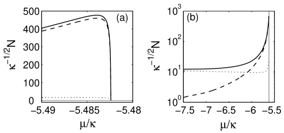
Figure 6: Bifurcation of the soliton solutions for two values of the zero-point energy difference: $\varepsilon=-5.30\kappa$ (panel (a)) and $\varepsilon_{\mathrm{cr}}=-5.45\kappa$ (panel (b)). The dimensionless units of system (13) are used. Here $a=0.001$. In both panels: the dotted lines correspond to $N_{u}$, the dashed to $N_{v}$, and the solid ones to the total number of atoms.

It is seen that the curves shown in fig. 6(b) indeed cease at the finite values $N_{u}=21$ and $N_{v}=670$ (according to equation (48)) on the boundary $\mu=\mu_{1}$ of the soliton existence. The corresponding soliton solutions are unstable as $\mu\to\mu_{1}$, as they correspond to the positive slope of the curve $N=N(\mu)$ for the total number of atoms. Solitons corresponding to fig. 6(a), on the contrary, are stable in this limit.

Moreover, for $\varepsilon<\varepsilon_{\mathrm{cr}}$, for values of the chemical potential close to the boundary $\mu_{1}$ there are soliton solutions which represent the unusual self-bound states of BEC, where almost all atoms are gathered in the repulsive $v$-condensate. The unusual solitons have the shape similar to that of soliton-(2) of fig. 4 and appear for small values of the parameter $a$. Indeed, their appearance is conditioned by $\varepsilon<0$ at least, according to formula (33), while the condition $a<1$ is necessary for a negative lower boundary $\varepsilon_{\mathrm{cr}}$. Obviously, the stability of such solitons is derived from the strong tunnel-coupling to the attractive $u$-condensate and the atoms can be thought as existing in the “superposition” of the repulsive and attractive pairs.

IV Conclusion

We have studied the solitons in BEC in a double-well trap with far-separated wells, when the atomic interaction is externally switched from attractive to repulsive in the condensate trapped in one of the wells.

First of all, there are soliton solutions with almost all atoms contained in the attractive condensate, which correspond to weak tunnel-coupling between the condensates in the two wells of the trap. In this case the attractive condensate serves as a spatially inhomogeneous source of atoms for the repulsive one, thus tailoring the repulsive condensate to the soliton form.

However, there are unusual stable solitons in the system, when almost all atoms are contained in the repulsive condensate. It is found that such soliton solutions appear for weak repulsion when the zero-point energy of the well with the repulsive condensate is lower than that of the attractive one but is above some critical value depending on the tunneling and interaction coefficients. The unusual solitons describe the condensates strongly coupled via the quantum tunneling, notwithstanding the fact that the tunneling coefficient is small. This apparent paradox is resolved by noticing that the tunneling probability is proportional to the number of atoms and that the total number of atoms increases with increase of the relative share of atoms in the repulsive condensate.

The ground state of the system corresponds to the soliton solution with the larger share of atoms contained in the attractive condensate. However, the solitons with the larger share of atoms in the repulsive condensate are stable, hence they can be experimentally observed.

Appendix A Wave functions with the localization property

Here we show that the inverse-proportionality relation (5) holds for the eigenfunctions corresponding to the quasi-degenerate energy levels in the double-well trap with weak tunneling through the barrier.

The weakly asymmetric double-well potential can be cast as $\mathcal{V}=\mathcal{V}_{S}(y)+\mathcal{V}_{A}(y)$, where $\mathcal{V}_{S}(-y)=\mathcal{V}_{S}(y)$ is the symmetric potential and $\mathcal{V}_{A}(-y)=-\mathcal{V}_{A}(y)$ is the perturbation. Under assumption (3) the eigenfunctions of the full Hamiltonian

$$\hat{H}=\hat{H}_{S}+\mathcal{V}_{A}(y)\equiv-\frac{\hbar^{2}}{2m}\frac{\mathrm{d}^{2}}{\mathrm{d}y^{2}}+\mathcal{V}_{S}(y)+\mathcal{V}_{A}(y),$$ (49)

corresponding to the shifted degenerate energy levels are given by a rotation of the wave functions $|0\rangle$ and $|1\rangle$ corresponding to the degenerate energy levels of the unperturbed Hamiltonian $\hat{H}_{S}$:

$$|\mathcal{E}_{0}\rangle=\frac{|0\rangle+\mathcal{A}|1\rangle}{\sqrt{1+\mathcal{A}^{2}}},\quad|\mathcal{E}_{1}\rangle=\frac{\mathcal{A}|0\rangle-|1\rangle}{\sqrt{1+\mathcal{A}^{2}}},\quad\mathcal{A}\equiv\frac{\Delta\mathcal{E}-\Delta E}{2K},$$ (50)

where $\Delta E=E_{1}-E_{0}$ and $\Delta\mathcal{E}=\mathcal{E}_{1}-\mathcal{E}_{0}$ is the energy spitting in the unperturbed and perturbed trap, respectively, and $K=\langle 0|\mathcal{V}_{A}|1\rangle$. The condition for equation (50) is $K\ll\hbar\omega_{\perp}$, where $\hbar\omega_{\perp}$ serves as an estimate on the energy gap $E_{2}-E_{1}$ in the double-well trap.

Equation (50) guarantees that if the inverse proportionality relation (5) holds for the symmetric double-well it also holds for the asymmetric one. This follows from a simple calculation:

$$\frac{\langle y_{-}|\mathcal{E}_{0}\rangle}{\langle y_{-}|\mathcal{E}_{1}\rangle}=\frac{\frac{\langle y_{-}|0\rangle}{\langle y_{-}|1\rangle}+\mathcal{A}}{\mathcal{A}\frac{\langle y_{-}|0\rangle}{\langle y_{-}|1\rangle}-1}=\frac{-\frac{\langle y_{+}|1\rangle}{\langle y_{+}|0\rangle}+\mathcal{A}}{-\mathcal{A}\frac{\langle y_{+}|1\rangle}{\langle y_{+}|0\rangle}-1}=-\frac{\langle y_{+}|\mathcal{E}_{1}\rangle}{\langle y_{+}|\mathcal{E}_{0}\rangle},$$ (51)

where the supposed inverse proportionality relation (5) for $|0\rangle$ and $|1\rangle$ have been used. On the other hand, under the assumption that the tunneling coefficient is weak the eigenfunctions of the symmetric double well are well-known combinations of the eigenfunctions for the two far-separated wells: $|0\rangle=(|\ell\rangle+|r\rangle)/\sqrt{2}$, $|1\rangle=(|\ell\rangle-|r\rangle)/\sqrt{2}$. Then the relation $\frac{\langle y_{-}|0\rangle}{\langle y_{-}|1\rangle}\approx-\frac{\langle y_{+}|1\rangle}{\langle y_{+}|0\rangle}\approx 1$ is obvious due to localization of the wave functions $|\ell\rangle$ and $|r\rangle$ in the respective wells and the symmetry. This concludes the proof of equation (5).

References

- (1) L. P. Pitaevskii, Zh. Eksp. Teor. Fiz. 40, 646 (1961) [Sov. Phys. JETP 13, 451 (1961); E. P. Gross, Nuovo Cimento 20, 454 (1961); J. Math. Phys. 4, 195 (1963). See also a review: F. Dalfovo, S. Giorgini, L. P. Pitaevskii, and S. Stringari, Reviews of Modern Physics, 71, 463 (1999).
- (2) M. R. Andrews, C. G. Townsend, H.-J. Miesner, D.S. Durfee, D. M. Kurn, and W. Ketterle, Science 275, 637 (1997).
- (3) D. S. Hall, M. R. Matthews, C. E. Wieman, and E. A. Cornell, Phys. Rev. Lett. 81, 1543 (1998).
- (4) A. Röhrl, M. Naraschewski, A. Schenzle, and H. Wallis, Phys. Rev. Lett. 78, 4143 (1997).
- (5) A. J. Leggett, Rev. Mod. Phys. 73, 307 (2001).
- (6) A. Hasegawa and Y. Kodama, Solitons in Optical Communications (Oxford University Press, Oxford, 1995).
- (7) S. Burger, K. Bongs, S. Dettmer, W. Ertmer, K. Sengstock, A. Sanpera, G. V. Shlyapnikov, and M. Lewenstein, Phys. Rev. Lett. 83, 5198 (1999).
- (8) J. Denschlag, J. E. Simsarian, D. L. Feder, C. W. Clark, L. A. Collins, J. Cubizolles, L. Deng, E. W. Hagley, K. Helmerson, W. P. Reinhardt, S. L. Rolston, B. I. Schneider, and W. D. Phillips, Science 287, 97 (2000).
- (9) B. P. Anderson, P. C. Haljan, C. A. Regal, D. L. Feder, L. A. Collins, C. W. Clark, and E. A. Cornell, Phys. Rev. Lett. 86, 2926 (2001).
- (10) S. Burger, L. D. Carr, P. Öhberg, K. Sengstock, and A. Sanpera, Phys. Rev. A 65, 043611 (2002).
- (11) K. E. Strecker, G. B. Partridge, A. G. Truscott, and R. G. Hulet, Nature 417, 150 (2002).
- (12) L. Khaykovich, F. Scheck, G. Ferrari, T. Bourdel, J. Cubizolles, L. D. Carr, Y. Castin, C. Salomon, Science 296, 1290 (2002).
- (13) A. J. Moerdijk, B. J. Verhaar, and A. Axelsson, Phys. Rev. A 51, 4852 (1995).
- (14) M. Wouters, J. Tempere, and J. T. Devreese, Phys. Rev. A 68, 053603 (2003).
- (15) K. V. Krutitsky, F. Burgbacher, and J. Audretsch, Phys. Rev. A 59, 1517 (1999). K. V. Krutitsky, K.-P. Marzlin, and J. Audretsch, Phys. Rev. A 65, 063609 (2002); Phys. Rev. A 67, 041606(R) (2003).
- (16) P. O. Fedichev, Y. Kagan, G. V. Shlyapnikov, and J. T. M. Walraven, Phys. Rev. Lett. 77, 2913 (1996).
- (17) J. L. Bohn and P. S. Julienne, Phys. Rev. A 56, 1486 (1997).
- (18) V. S. Shchesnovich, B. A. Malomed, and R. A. Kraenkel, Physica D (2003), in press.
- (19) A. Smerzi, S. Fantoni, S. Giovanazzi, and S. R. Shenoy, Phys. Rev. Lett. 79, 4950 (1997).
- (20) S. Raghavan, A. Smerzi, S. Fantoni, and S. R. Shenoy, Phys. Rev. A 59, 620 (1999).
- (21) G. J. Milburn, J. Corney, E. M. Wright, and D. F. Walls, Phys. Rev. A 55 4318 (1997).
- (22) G. Kalosakas, A. R. Bishop, and V. M. Kenkre, Physical Review A 68, 023602 (2003).
- (23) E. A. Ostrovskaya, Yu. S. Kivshar, M. Lisak, B. Hall, F. Cattani, and D. Anderson, Phys. Rev. A 61, 031601 (2000).
- (24) P. Coullet and N. Vandenberghe, J. Phys. B: At. Mol. Opt. Phys. 35, 1593 (2002).
- (25) B. Fornberg, A Practical Guide to Pseudospectral Methods (Cambridge University Press, Cambridge, UK, 1996); J. P. Boyd, Chebyshev and Fourier Spectral Methods, Second Edition (DOVER Publications, Inc., New York, 2000); L. N. Trefethen, Spectral Methods in Matlab (SIAM, Philadelphia, PA, 2000).
- (26) G. P. Berman, A. Smerzi, and A. R. Bishop, Phys. Rev. Lett. 88, 120402 (2002).
- (27) J. M. Soto-Crespo and N. Akhmediev, Phys. Rev. E 48, 4710 (1993).
- (28) N. Akhmediev and A. Ankiewicz, Phys. Rev. Lett. 70, 2395 (1993).
- (29) B.A. Malomed, Progr. Optics 43, 69 (2002).
- (30) M. G. Vakhitov and A. A. Kolokolov, Radiophys. Quant. Electron. 16, 783 (1975).
- (31) E. A. Kuznetsov, A. M. Rubenchick, and V. E. Zakharov, Phys. Rep. 142, 103 (1986).
- (32) A. Gammal, T. Frederico, and L. Tomio, Phys. Rev. A 64, 055602 (2001)