Largest Lyapunov exponent of long-range XY systems

Abstract

We calculate analytically the largest Lyapunov exponent of the so-called $\alpha XY$ Hamiltonian in the high energy regime. This system consists of a $d$-dimensional lattice of classical spins with interactions that decay with distance following a power-law, the range being adjustable. In disordered regimes the Lyapunov exponent can be easily estimated by means of the “stochastic approach”, a theoretical scheme based on van Kampen’s cumulant expansion. The stochastic approach expresses the Lyapunov exponent as a function of a few statistical properties of the Hessian matrix of the interaction that can be calculated as suitable microcanonical averages. We have verified that there is a very good agreement between theory and numerical simulations.

and

1 Introduction

The largest Lyapunov exponent (LLE) measures the sensitivity to initial conditions in dynamical systems. More precisely, it gives the asymptotic rate of exponential growth of most vectors in tangent space. Thus, the determination of the LLE, either numerical or analytical, requires the knowledge of the long-time behavior of a system of linear differential equations with time-dependent coefficients.

From a numerical point of view, there are standard and simple algorithms for computing the LLE that perform satisfactorily, even for large systems [1]. To the best of our knowledge, the first attempt to evaluate analytically the LLE of many-body systems with smooth Hamiltonians was made by Pettini and collaborators, less than ten years ago [2, 3]. This “geometric” approach begins by postulating a mean-field approximation in tangent space. Then, the few resulting equations are handled with the techniques of stochastic differential equations (cumulant expansion [4]) which, eventually, lead to an analytical estimate of the LLE. Despite the success of the geometric method in reproducing the LLE of some many-particle systems, it must be stressed that, from a theoretical point of view, this method is unsatisfactory: it presents drawbacks such as ad-hoc approximations, ill-defined ingredients, and free parameters (see the discussion in Ref. [5]). However, it is possible to construct a first-principles theory following the steps of Pettini et al., but avoiding the defects of the geometric method. The idea is simple: do not invoke a mean-field approximation at the start, just apply the cumulant expansion to the full $N$-particle problem. This recipe was partially executed by Barnett et al. [6] and then complemented by the present authors [5]. The result is a theory where all the ingredients are well defined, there are no free parameters, and approximations are controllable. Even if several of these approximations are really crude, it was shown [7] that the theory is still capable of quantitative predictions.

Reference [7] contains the application of the “stochastic approach” to the disordered regimes of the infinite-range $XY$ Hamiltonian (HMF) [8, 9]. This model consists of a $d$-dimensional lattice of classical spins rotating in parallel planes, and with a pairwise interaction that depends on the relative orientation of spins but not on the distance between them. In Ref. [10] the HMF was generalized by making the interaction depend on the distance $r$ according to the power law $r^{-\alpha}$, thus obtaining the family $\alpha XY$ (the case $\alpha=0$ recovers the HMF, $\alpha/d\to\infty$ corresponds to first neighbors interactions). The purpose of this paper is to estimate analytically the LLE of the disordered regimes of the $\alpha XY$ family, using the stochastic approach [7]. The restriction to these regimes is not an intrinsic limitation of the theory but obeys to the general technical difficulty of determining two-time correlation functions. In the disordered regimes of the $\alpha XY$ models the relevant correlation functions are approximately Gaussian.

The rest of the paper is organized as follows. For reasons of self-containedness, we begin by presenting a very short review of the theory in Sect. 2. The systems to be studied (the $\alpha XY$ Hamiltonians) are introduced in Sect. 3, where we also work out the predictions of the theory for these particular systems. Section 4 contains the critical comparison of theoretical results with numerical simulations. We close in Sect. 5 with a summary and some remarks.

2 A short review of the theory

We consider Hamiltonians of the type

$${\mathcal{H}}=\frac{1}{2}\sum_{i=1}^{N}p^{2}_{i}+{\mathcal{V}}(q_{1},\ldots,q_{N}),$$ (1)

where $q_{i}$ and $p_{i}$ are conjugate coordinates, and the interaction potential ${\mathcal{V}}$ is assumed to be small. This is the case of the disordered phases of the $\alpha XY$ models where the interaction energy is very small as compared to the kinetic energy. Let us denote phase space points by $x$ and tangent vectors by $\xi$. Differentiating the Hamilton equations, one obtains the evolution equations for tangent vectors:

$$\dot{\xi}={\bf A}(t)\,\xi.$$ (2)

For a Hamiltonian of the special form (1), the operator $\bf A$ has the simple structure

$${\bf A}(t)=\left(\matrix{0&{\bf 1}\cr-{\bf V}(t)&0}\right)\;.$$ (3)

Here $\bf V$ is the Hessian matrix of the potential ${\mathcal{V}}$, namely $V_{ij}=\partial^{2}\mathcal{V}/\partial q_{i}\partial q_{j}.$ Once initial conditions $x_{0}$ and $\xi_{0}$ have been specified, the LLE $\lambda$ can be found by calculating the limit [1]

$$\lambda=\lim_{t\to\infty}\frac{1}{2t}\ln|\xi(t;x_{0},\xi_{0})|^{2}\;.$$ (4)

We assume that for any initial condition $x_{0}$ in phase space, the trajectory $x(t;x_{0})$ is ergodic on its energy shell. This implies that $\lambda$ depends only on energy and other system parameters, but not on $x_{0}$, which can then be chosen randomly according to the microcanonical distribution. There will also be no dependence on initial tangent vectors, because if $\xi_{0}$ is also chosen randomly, it will have a non-zero component along the most expanding direction. Moreover, assuming weak intermittency, one can write

$$\lambda\approx\lim_{t\to\infty}\frac{1}{2t}\ln\left\langle|\xi(t;x_{0},\xi_{0})|^{2}\right\rangle\;,$$ (5)

brackets meaning microcanonical averages over $x_{0}$. This is our first approximation, to be discussed in Sect. 5.

By letting $x_{0}$ be a random variable, ${\bf V}(t;x_{0})$ becomes a stochastic process, and Eq. (2) can be treated as a stochastic differential equation. However, as we are interested in the square of the norm of $\xi$, we focus, not on Eq. (2) itself, but in the related equation for the evolution of the “density matrix” $\xi\xi^{T}$:

$$\frac{\rm d}{{\rm d}t}(\xi\xi^{T})={\bf A}\xi\xi^{T}+\xi\xi^{T}{\bf A}^{T}\equiv\hat{\bf A}\xi\xi^{T},$$ (6)

the rightmost identity defining the linear superoperator $\hat{\bf A}$. For the purpose of the perturbative approximations to be done, the operator $\hat{\bf A}$ is split into two parts $\hat{\bf A}=\hat{\bf A}_{0}+\hat{\bf A}_{1}(t)$, where $\hat{\bf A}_{0}$ corresponds to the evolution in the absence of interactions, and $\hat{\bf A}_{1}$ depends on the Hessian of the interaction. Assuming that the fluctuations of ${\bf A}_{1}(t)$ are small and/or rapid enough, it is possible to manipulate Eq. (6) to derive an explicit expression for the evolution of the average of $\xi\xi^{T}$:

$$\langle{\xi\xi^{T}}\rangle(t)=\exp\left({t\hat{\bf\Lambda}}\right)\;{\xi_{0}\xi_{0}^{T}}\;,$$ (7)

where $\hat{\bf\Lambda}$ is a time-independent superoperator given by a cumulant expansion, which we truncate at the second order (the lowest non-trivial order). We refer the reader to [4, 5] for explicit expressions. The truncation of the cumulant expansion is our second approximation. The perturbative parameter controlling the quality of the truncation is the product of two quantities, the “Kubo number” $\sigma\tau_{c}$. The first factor, $\sigma$, characterizes the amplitude of the fluctuations of $\hat{\bf A}_{1}(t)$. The second, $\tau_{c}$, is the correlation time of $\hat{\bf A}_{1}(t)$.

Let $L_{\rm max}$ be the eigenvalue of $\hat{\bf\Lambda}$ which has the largest real part. Taking the trace of Eq. (7), one sees that the LLE $\lambda$ is related to the real part of $L_{\rm max}$ by

$$\lambda=\mbox{$\frac{1}{2}$}\,\mbox{Re}\,\left(L_{\rm max}\right)\;.$$ (8)

To proceed further one needs the matrix of $\hat{\bf\Lambda}$ in some basis. The crudest approximation consists in restricting $\hat{\bf\Lambda}$ to a particular three-dimensional subspace, a choice that is equivalent to a mean-field approximation in tangent space [5]. The corresponding 3$\times$3 matrix for $\hat{\bf\Lambda}$ is:

$${\bf\Lambda}=\left(\matrix{0&0&2\cr 2\sigma^{2}\tau_{c}^{(1)}&-2\sigma^{2}\tau_{c}^{(3)}&-2\mu\cr-\mu+2\sigma^{2}\tau_{c}^{(2)}&1&-2\sigma^{2}\tau_{c}^{(3)}\cr}\right)\;,$$ (9)

with the definitions

$$\mu = \frac{1}{N}{\rm Tr}\langle{\bf V}\rangle\;,\quad\sigma^{2}=\frac{1}{N}{\rm Tr}\langle\left(\delta{\bf V}\right)^{2}\rangle\;,$$ (10)

$$\tau_{c}^{(k+1)} = \int_{0}^{\infty}d\tau\,\tau^{k}f(\tau)\;,\quad f(\tau)=\frac{1}{N\sigma^{2}}{\rm Tr}\langle\delta{\bf V}(0)\delta{\bf V}(\tau)\rangle$$ (11)

(see [5, 7] for details). In the mean-field approximation the LLE is expressed in terms of the set of four parameters $\mu$ and $\sigma^{2}\tau_{c}^{(k+1)}$, $k=0,1,2$. The parameters $\mu$ and $\sigma$ are, respectively, the mean and variance of the stochastic process ${\bf V}(t)$. The characteristic time $\tau_{c}^{(1)}\equiv\tau_{c}$ is naturally interpreted as the correlation time of the process ${\bf V}(t)$, $f(\tau)$ being the relevant correlation function.

3 The $\alpha XY$ Hamiltonians

In this section we apply the perturbative/mean-field theory of Sect. 2 to the $\alpha XY$ Hamiltonians

$$H=\frac{1}{2}\sum_{i=1}^{N}p_{i}^{2}+\frac{J}{2\tilde{N}}\sum_{i,j=1}^{N}\frac{1-\cos(\theta_{i}-\theta_{j})}{r_{ij}^{\alpha}}\equiv{\mathcal{K}}+{\mathcal{V}}\;,$$ (12)

where $\tilde{N}=\tilde{N}(\alpha,d)=\sum_{ij}r_{ij}^{-\alpha}/N$, and $r_{ij}$ is the distance on the periodic lattice [10]. This model represents a lattice of classical spins with the interaction range controlled by the parameter $\alpha$. Each spin rotates in a plane and is therefore described by an angle $0\leq\theta_{i}<2\pi$, and its conjugate angular momentum $p_{i}$, with $i=1,\ldots,N$. The constant $J>0$ is the interaction strength. The $\alpha XY$ Hamiltonian has been extensively studied in the last few years. It has been shown that the long-range cases ($\alpha<d$) have the same thermodynamic properties as the $\alpha=0$ case (HMF), in all the energy range [11, 12]. If one looks only at the high energy regimes, then for all $\alpha$ the equilibrium properties are those of a gas of almost free rotators. However, time scales do depend on $\alpha$. This is the case of LLEs, which have been studied in detail, both numerically [10] and analytically. Scaling laws for high energies were obtained by Firpo and Ruffo [13], using the geometric method [2, 3] and also by the present authors, using a random-matrix approach [14].

In order to apply the stochastic approach, in its mean-field second-order-perturbative version, one has to calculate the average, variance, and correlation function of the Hessian ${\bf V}(t)$, i.e., Eqs. (10) and (11). For high energies these ingredients can be easily estimated, using simple approximations. Anyway, we will verify that the theoretical estimates, coarse as they are, coincide with the exact time averages calculated numerically.

The elements of the matrix ${\bf V}$ can be readily obtained:

$$V_{ij}=-\frac{J}{\tilde{N}}\frac{\cos(\theta_{i}-\theta_{j})}{r_{ij}^{\alpha}}\;\;(i\neq j)\;;\quad V_{ii}=-\sum_{j\neq i}V_{ij}\;.$$ (13)

Then, inserting this result in the definition (10) of $\mu$ we arrive at $\mu/J=1-2\langle{\mathcal{V}}\rangle/(NJ)$. The average potential energy $\langle{\mathcal{V}}\rangle$ can be calculated as a canonical average following the (now standard) saddle-point calculations of Refs. [12, 13]. Skipping the details, one arrives at

$$\mu/J\approx\frac{\beta J}{2}\frac{\tilde{N}(2\alpha,d)}{{\tilde{N}}^{2}(\alpha,d)}\equiv\frac{\beta J}{2}\frac{1}{{\mathcal{N}}(\alpha,d)}\;,$$ (14)

where $\beta$, the inverse of the temperature, is related to the energy per particle $\varepsilon$ through $\beta^{-1}=2\varepsilon-J$, in the disordered regimes. This expression for $\mu$ coincides with the result obtained by Firpo and Ruffo [13], except for a factor of two.

The calculation of $\sigma^{2}$ proceeds in the same way as in the case $\alpha=0$ (see [7]), but here we make the extreme approximation of free rotators. That is, we assume

$$\langle\cos(\theta_{i}-\theta_{j})\rangle \approx 0\;,$$

$$\langle\cos^{2}(\theta_{i}-\theta_{j})\rangle \approx 1/2\;,$$

$$\langle\cos(\theta_{i}-\theta_{j})\cos(\theta_{i}-\theta_{k})\rangle \approx 0\;,$$ (15)

where it is understood that $i\neq j$ and $j\neq k$. Then the final approximate expression for $\sigma^{2}$ is

$$\sigma^{2}\approx J^{2}\frac{1}{{\mathcal{N}}(\alpha,d)}\;.$$ (16)

At high temperatures, the relative importance of the interactions decreases with increasing energy and $N$, and the dynamics is dominated by the kinetic part of the Hamiltonian. The picture is that of particles rotating almost freely during times which are long as compared to the mean rotation period. For any value of $\alpha$ we can assume, as a first approximation, that the values of $\{\theta_{k}\}$ and $\{p_{k}\}$ are independent random variables with uniform and Maxwell distributions, respectively. The decorrelation mechanism is just single-particle phase mixing. Within this approximation the correlation function is Gaussian and the correlation time is of the order of the mean period of rotation, i.e., [7]

$$\tau_{c}\sim\sqrt{\frac{\pi\beta}{4}}\;.$$ (17)

Gathering the results of previous sections, one can construct the $3\times 3$ matrix ${\bf\Lambda}$, and extract the LLE from the eigenvalue of ${\bf\Lambda}$ with the largest real part. However, we have verified that for the cases considered here, the LLE is very well approximated by the asymptotic expression [7]

$$\lambda\approx\left(\frac{\sigma^{2}\tau_{c}}{2}\right)^{1/3}\;,$$ (18)

with $\sigma^{2}$ and $\tau_{c}$ given by Eqs. (16) and (17). The absence of $\mu$ in the leading-order expression for $\lambda$ says that in the disordered phases of the $\alpha XY$, fluctuations are much larger than the average, i.e. $\sigma\gg\mu$, and dominate the tangent dynamics. We conclude this section by noting that Eq. (18) leads to the same scaling laws obtained in Refs. [13, 14].

4 Numerical studies

First of all we verified that the analytical calculations of $\mu$, $\sigma^{2}$, and $\tau_{c}$ agree with the corresponding dynamical averages. This test was perfomed for the case $d=1$. In Fig. 1 we show numerical values for $\mu$ and $\sigma^{2}$ for various values of $\alpha$. Numerical integration of the equations of motion was performed using a fourth order symplectic algorithm [15], with equilibrium initial conditions, i.e., angles uniformly distributed in $[0,2\pi)$ and Gaussian distribution of momenta. Forces were calculated using a Fast Fourier Transform algorithm. One sees that the numerical data can be well described by the approximate expressions (14) and (16).

Figure 1: Numerical (symbols) and analytical (lines) values of $\mu$, $\sigma^{2}$, and $\tau_{c}$ for the $\alpha XY$ model as functions of the interaction range $\alpha$ ($d=1$). Energy is fixed at $\varepsilon=5.0$, $J=1$ and system size is $N=128$ (circles) or $N=512$ (squares). Error bars (not shown) are of the order of the symbol size.

In order to discuss the correlation times, let us now look at the correlation functions of Fig. 2. Theory and simulations agree almost perfectly in the central part of the distributions. However, there are long tails that grow with increasing $\alpha$. We recall that the quantities $\tau^{(k)}$ are moments of the correlation function $f(\tau)$, and as such, very sensitive to the precise shape of the tails. So, as $\alpha$ grows, we lose confidence on the Gaussian estimates for $\tau^{(k)}$.

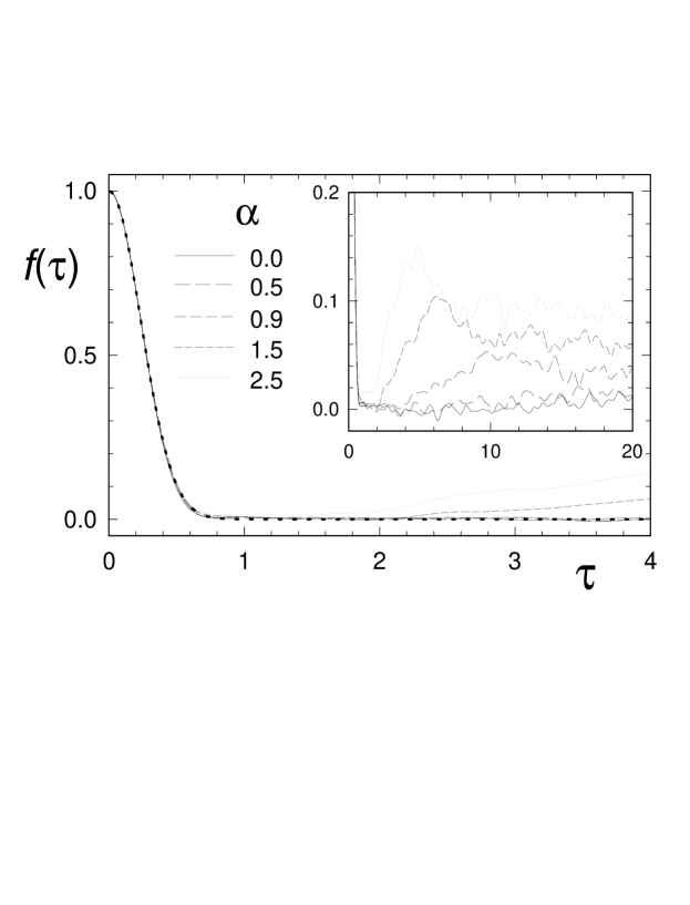
Figure 2: Correlation functions for $N=256$, $\varepsilon=5.0$ and $J=1$. Several values of $\alpha$ are considered ($d=1$). We have averaged over 100 initial conditions. The dotted line is our theoretical prediction (a Gaussian). The inset shows that tail fluctuations grow with $\alpha$.

For comparing the theory with simulations, we will use LLE data existing in the literature [10, 16]. Figure 3 shows LLEs for different values of $\alpha$ as a function of the system size and $\varepsilon=5.0$. We have considered large particle numbers $(N\geq 50)$ and an energy well above the transition to ensure (i) the validity of the approximations invoked in calculating the averages of Sect. 3, and also (ii) to guarantee that we are in a disordered, quasi-ballistic regime. Full lines correspond to the theoretical LLEs obtained by using the asymptotic expression of Eq. (18). Figure 3 shows a satisfactory agreement between theory and simulations. Differences in the definition of $\tilde{N}$ were absorbed in $J$, otherwise set equal to one.

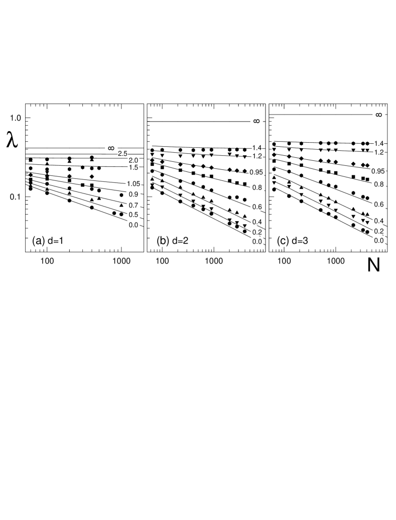
Figure 3: Largest Lyapunov exponent of the $\alpha XY$ Hamiltonians as a function of system size $N$, interaction range $\alpha$ and lattice dimension $d$. Energy is fixed at $\varepsilon=5.0$. Symbols correspond to numerical data in the literature for $d=1$ [10] and $d=2,3$ [16]. Lines are our theoretical predictions, labeled by the ratio $\alpha/d$.

5 Summary and concluding remarks

In a previous paper we had seen that the stochastic recipe works satisfactorily in the quasi-ballistic regimes of the HMF ($\alpha=0$). Now we have verified that the theory still works well when the interaction range is not infinite. Even for short-range interactions we have found a good agreement between theory and simulations. This suggests that the crude approximations that allowed us to estimate the LLE may be reasonable in these cases. Let us summarize the approximations we used.

First of all we invoked a weak intermittency approximation to exchange logarithm and average. We tested this approximation in the $\alpha=0$ case [7] and verified that it does not introduce an important error (about or less than 10%, for the cases considered). Even though we have not made numerical tests for $\alpha>0$, we suspect that intermittency does not increase with $\alpha$, one reason being that the system becomes more chaotic with increasing $\alpha$ (the LLE grows with $\alpha$).

The second approximation, and most important one, is the truncation of the cumulant expansion at the second order. By doing so, one introduces a relative error of the order of the Kubo number $\sigma\tau_{c}$. This perturbative parameter grows with $\alpha/d$ but saturates at a finite value as $\alpha\to\infty$ (as illustrated in Fig. 1 for $d=1$), so there are no indications that the cumulant expansion may fail for short-range.

The “mean-field” diagonalization is exact in the infinite-range case [5] and was expected to be a good approximation for long-range interactions ($\alpha<d$). For short-range forces, this approximation represents a crude truncation of the basis for diagonalizing $\hat{\Lambda}$. Note however that we are dealing with a Hermitian problem, i.e., finding the largest eigenvalue of $\langle\xi\xi^{T}\rangle(t)$ [Eq. (7)], then, if $\hat{\Lambda}$ is calculated accurately, truncation of the basis may still produce a good lower bound to the LLE. This could be the explanation for the agreement between theory and simulations also for $\alpha>d$ (see Fig. 3). However, this accord should be further explored and tested for values of $\alpha$ larger than those here considered.

We have limited our presentation to equilibrium situations. If the system does not explore the full phase space, as is the case of the quasi-stationary regimes of the $\alpha XY$ [17], the stochastic method may still be applied, but then one has to replace microcanonical averages by averages over the (a priori unknown) regions of phase space that are effectively visited by the system.

We are grateful to A. Campa, A. Giansanti, D. Moroni and C. Tsallis for communicating their numerical data. We acknowledge Brazilian Agencies CNPq, FAPERJ and PRONEX for financial support.

References

- [1] G. Benettin, L. Galgani, and J.-M. Strelcyn, Phys. Rev. A. 14, 2338 (1976).
- [2] L. Casetti, M. Pettini and E. G. D. Cohen, Phys. Rep. 337, 238 (2000).
- [3] L. Casetti, C. Clementi and M. Pettini, Phys. Rev. E 54, 5969 (1996).
- [4] N. G. van Kampen, Phys. Rep. 24, 171 (1976); Stochastic Processes in Physics and Chemistry (North-Holland, Amsterdam, 1981).
- [5] R. O. Vallejos and C. Anteneodo, Phys. Rev. E 66, 021110 (2002).
- [6] D. M. Barnett, T. Tajima, K. Nishihara, Y. Ueshima, and H. Furukawa, Phys. Rev. Lett. 76, 1812 (1996) and Phys. Rev. E 55, 3439 (1997).
- [7] C. Anteneodo, R. N. P. Maia, and R. O. Vallejos, Phys. Rev. E 68, 036120 (2003).
- [8] M. Antoni and S. Ruffo, Phys. Rev. E 52, 2361 (1995).
- [9] T. Dauxois, V. Latora, A. Rapisarda, S. Ruffo, and A. Torcini, in Dynamics and Thermodynamics of Systems with Long Range Interactions, Lecture Notes in Physics Vol. 602 (Springer, Heidelberg, 2002).
- [10] C. Anteneodo and C. Tsallis, Phys. Rev. Lett. 80, 5313 (1998).
- [11] F. Tamarit and C. Anteneodo, Phys. Rev. Lett. 84, 208 (2000).
- [12] A. Campa, A. Giansanti and D. Moroni, Phys. Rev. E 62, 303 (2000).
- [13] M.-C. Firpo and S. Ruffo, Phys. Lett. A 34, L511 (2001).
- [14] C. Anteneodo and R. O. Vallejos, Phys. Rev. E 65, 016210 (2001).
- [15] H. Yoshida, Phys. Lett. A 150, 262 (1990).
- [16] A. Giansanti, D. Moroni and A. Campa, Chaos, Solitons and Fractals 13, 407 (2002); A. Campa, A. Giansanti, D. Moroni and C. Tsallis, Phys. Lett. A 286, 251 (2001).
- [17] V. Latora, A. Rapisarda and C. Tsallis, Phys. Rev. E 64, 056134 (2001); B.J.C. Cabral and C. Tsallis, Phys. Rev. E 66, 065101 (2002).