Stimulated and spontaneous relaxation in glassy systems

Abstract

Recent numerical simulations of a disordered system [5] have shown the existence of two different relaxational processes (called stimulated and spontaneous) characterizing the relaxation observed in structural glasses. The existence of these two processes has been claimed to be at the roots of the intermittency phenomenon observed in recent experiments. Here we consider a generic system put in contact with a bath at temperature $T$ and characterized by an adiabatic slow relaxation (i.e. by a negligible net heat flow from the system to the bath) in the aging state. We focus on a simplified scenario (termed as partial equilibration) characterized by the fact that $T=0$ (where only the spontaneous process is observable) and whose microscopic stochastic dynamics is ergodic when constrained to the constant energy surface. Three different effective temperatures can be defined: a) from the fluctuation-dissipation theorem (FDT), $T_{\rm eff}^{\rm FDR}$, b) from a fluctuation theorem describing the statistical distribution of heat exchange events between system and bath, $T_{\rm eff}^{\rm FT}$ and c) from a set of observable-dependent microcanonical relations in the aging state, $T_{\rm eff}^{\rm MR}$. In a partial equilibration scenario we show how all three temperatures coincide reinforcing the idea that a statistical (rather than thermometric) definition of a non-equilibrium temperature is physically meaningful in aging systems. These results are explicitly checked in a simple model system.

1 Introduction

Efforts to extend well established concepts in equilibrium thermodynamics to the non-equilibrium domain have repeatedly appeared many times in the past in different contexts. An idea that has attracted the attention of physicists for quite a long time is the concept of a temperature applied to non-equilibrium states [1]. In equilibrium, the notion of temperature can be covered from two different perspectives. On the one hand, there is the thermodynamic approach where temperature is defined as a parameter that characterizes classes of systems in mutual thermal equilibrium. The usefulness of this thermometric definition relies on the validity of the zeroth law of thermodynamics. On the other hand, there is a statistical approach (ensemble theory) where temperature can be defined from the properties of individual systems without any reference to the mutual equilibrium property. The statistical temperature is defined as the inverse of the energy gradient of the configurational entropy measured over a constant energy surface. The maximum entropy postulate relates the statistical notion of the temperature to the thermometric one. The statistical and thermodynamic concepts look equivalent but they are not as the latter requires a specific behavior of the different systems when put in mutual contact. The thermodynamic definition of a temperature represents a stronger condition than the statistical one.

An interesting category of systems that has recently received considerable attention are glassy systems in their aging regime. The aging regime is a slow relaxational process characterized by the extremely small net amount of heat delivered by the system to the bath in contact. It has been suggested [2] that in aging systems a thermometric definition of non-equilibrium temperature is meaningful for a thermometer responding to low-enough frequencies. We suspect that this definition is too strong and might be wise to investigate a low-level statistical definition of a non-equilibrium temperature.

The purpose of this paper is to show that a statistical definition of non-equilibrium or effective temperature (rather than thermometric) can be rescued for a particular category of aging systems characterized by adiabatic slow relaxation. In this category of systems relaxation is imposed to be ergodic when constrained to a given energy shell. At $T=0$ this condition defines what we term as partial equilibration scenario. For this class of systems three different definitions of an effective temperature are possible: a) from the fluctuation-dissipation theorem (FDT), $T_{\rm eff}^{\rm FDR}$; b) from the fluctuation theorem applied to the statistical distribution of heat exchange events between system and bath, $T_{\rm eff}^{\rm FT}$; c) from a set of microcanonical relations in the aging state, $T_{\rm eff}^{\rm MR}$. In a partial equilibration scenario we show how all these temperatures coincide reinforcing the idea that a statistical definition of a non-equilibrium temperature is physically meaningful in aging systems. We check all statements and results in a simple model of glassy system where the partial equilibration scenario holds and explicit computations can be done.

2 Adiabatic relaxation

Let us consider a system that is prepared in a non-equilibrium state by placing it in contact with a thermal bath at low temperature (quenching protocol). The system will relax and release heat to the bath in a process that can span from several minutes to millions of years. Only when the system has reached equilibrium the net heat current from the system to the bath vanishes. All along the paper we will refer to this relaxational regime as the aging regime and the corresponding non-equilibrium state as the aging state. The time after the quench will be referred as the age of the system and will be denoted by one or two of the variables $s$ and $t$ depending on whether one-time or two-time quantities quantities are considered. We adopt the convention $t>s$.

Several definitions and quantities seem appropriate to put the discussion in perspective . Let us consider a system described by an energy function $E({\cal C})$ where ${\cal C}$ denotes a generic configuration. The system is in contact with a thermal bath and the microscopic stochastic dynamics is both ergodic and satisfies the detailed balance property. $P_{t}({\cal C})$ will denote the probability for the system to be in the configuration ${\cal C}$ at time $t$. The average value of an observable $A$ at time $t$ will be denoted by $A(t)$ and is given by,

$$A(t)=\sum_{{\cal C}}A({\cal C})P_{t}({\cal C})~{}~{}~{}.$$ (1)

Often the time argument in $A(t)$ will be dropped off and we will simply write $A$, with the clear understanding that in general it is a time-varying quantity. $P({\cal C^{\prime}},t|{\cal C},s)$ denotes the conditional or transition probability for the system to be at configuration ${\cal C^{\prime}}$ at time $t$ if it was at configuration ${\cal C^{\prime}}$ at time $s$. The autocorrelation ($C_{A}(t,s)$) and response ($R_{A}(t,s)$) functions are defined by,

$$C_{A}(t,s)=\sum_{{\cal C},{\cal C^{\prime}}}P({\cal C^{\prime}},t|{\cal C},s)A({\cal C})A({\cal C^{\prime}})~{}~{}~{}~{}~{}~{}~{};~{}~{}~{}~{}~{}~{}~{}R_{A}(t,s)=\frac{\delta\langle A(t)\rangle}{\delta h(s)}$$ (2)

Both $C_{A}$ and $R_{A}$ can be decomposed into a stationary (fast) and aging (slow) parts. In the large $s$ regime, for many aging systems a quasi-FDT relates the aging parts of (2) in terms of the fluctuation-dissipation ratio (FDR),

$$R_{A}^{\rm ag}(t,s)=\frac{1}{T_{\rm eff}^{{\rm FDR}}(s)}\frac{\partial C_{A}^{\rm ag}(t,s)}{\partial s}\theta(t-s)~{}~{}~{}.$$ (3)

$T_{\rm eff}^{{\rm FDR}}(s)$ is a time-dependent effective temperature that has been shown to have some of the properties of a thermodynamic temperature [2]. In a weak ergodicity breaking scenario $C_{A}(t,s)$ decays to zero for $t-s\to\infty$ in a typical time that we denote by $\tau_{\rm decorr}(s)$ . In general, $\tau_{\rm decorr}(s)\propto s^{\alpha}$ with $\alpha$ a given exponent. In many cases $\alpha=1$ appears to be a very good approximation, usually termed as simple aging.

We define the aging regime as adiabatic if the fraction of heat released from the system to the bath goes asymptotically to zero for time differences of order of the decorrelation time,

$$\Biggl{|}\frac{E(s+\tau_{\rm decorr}(s))-E(s)}{E(s)}\Biggr{|}\to 0~{}~{}~{}~{}~{}{\rm for}\,\,s\,\,{\rm large\,\,enough}$$ (4)

Of course this relation is meaningful only in the aging regime where the energy $E(s)$ is still far from its equilibrium value . The relation between the rate decay of the energy and the frequency domain where FDT violations are observed has been already pointed out in [4].

3 Stimulated and spontaneous relaxation as the origin of intermittency.

For an adiabatic regime as described in (4) two type of heat exchange processes are predicted to be observable depending on the timescale of the measurement. According to (4), and for times of the order of $\tau_{\rm decorr}(s)$ or smaller, the net heat flow transferred from the system to the bath is exceedingly small, yet heat fluctuations can be as big as if the system were in equilibrium at the bath temperature. In such case there is a continuous heat exchange between the system and the bath and energy fluctuations $<E^{2}(s)>-<E(s)>^{2}$ (measured over $\tau_{\rm decorr}(s)$) are of the same order of the energy content $E(s)$ and determined by the heat capacity of the system at the bath temperature. Were one to measure at age $s$ the probability distribution $P_{s}(Q)$ of heat exchanged $Q$ between the system and the bath along intervals of a given duration $\tau\sim\tau_{\rm decorr}(s)$, a Gaussian distribution would be found with zero mean (as no net heat is transferred from the system to the bath) and a variance $\sigma^{2}(T)$ which is independent of the age $s$ but dependent on the temperature of the bath. This feature is ubiquitous in glassy matter (e.g. structural glasses quenched at low-enough temperatures) where the net heat flow from the system to the bath is unobservable, yet heat is quickly exchanged with the bath as thermal conductivity is high . For all practical purposes the system looks equilibrated at the temperature of the bath and a thermometer put in contact with it would measure the bath temperature. We call this heat exchange process stimulated as it originates in the existence of physical processes thermally excited by the bath.

For times much larger than $\tau_{\rm decorr}(s)$ the average net heat flow from the system to the bath is not negligible, a clear consequence that the system has not yet equilibrated. Most of the exchange processes that occur along these timescales are stimulated by the bath, however other exchange events do not fall into the previous category and follow a completely different distribution. Contrarily to the stimulated process, this distribution is expected to display an exponential tail whose width $\lambda(s)$ depends on the age of the system $s$. However this process is not excluded to be described by a Gaussian distribution as well. Indeed an exponential tail is characteristic of Gaussian distributions centered around a finite value. We call this new process spontaneous as its statistical description is not determined by the temperature of the bath but rather by the fact that the system has been prepared in a non-equilibrium state. Figure 1 illustrates typical distributions for the stimulated and spontaneous processes. The existence of two different kinds of heat exchange process (and therefore two different heat exchange distributions) occurring along widely separated timescales has been recently numerically verified in the context of a simple spin-glass model [5]. It has been suggested that the existence of these two processes is at the roots of the intermittency phenomenon observed in glasses [6] and colloids [7] .

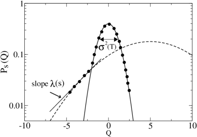
Figure 1: The origin of intermittency: Two mechanisms of relaxation, stimulated (continuous line) and spontaneous (dashed line) characterize the overall relaxation. $Q$ stands for the heat transferred from the bath to the system (the sign indicating the direction of flow, if $Q<0$ heat flows from the system to the bath) along regularly spaced time intervals and $P_{s}(Q)$ the corresponding probability distribution at age $s$. The black points illustrate what experimental measured data would look like. In the simplest scenario both processes are described by a Gaussian distribution. The stimulated component has a variance $\sigma^{2}(T)$ dependent on the bath temperature but independent on the age. The spontaneous component shows an exponential tail in the $Q<0$ side (shown as a continuous line) whose slope $\lambda$ is age dependent. The spontaneous process for $Q>0$ is unobservable as relaxational dynamics is constrained by the existence of a net heat transfer from the system to the bath.

4 Statistical (microcanonical) description of the aging state

Along the rest of the paper we will analyze in detail and idealized particular case of the more general previous scenario. In doing this we aim to understand fundamental issues behind a possible statistical, rather thermodynamical, description of the glassy state. We will consider in detail a situation where the stimulated process does not exist and only the spontaneous process is observed in the adiabatic relaxation. We will refer to it as the partial equilibration scenario. It is then possible to prove that effective temperatures, with a precise statistical meaning, do emerge. This is the content of the next Subsections, 4.1,4.2,4.3. In Sec. 5 we will focus our attention on the oscillator model (OM) [8] as a simple case where all results of the current Section can be explicitly verified.

4.1 Partial equilibration scenario

To suppress the stimulated process the bath is put at zero temperature (therefore, no heat can flow from the bath to the system). However, to keep the system in an adiabatic relaxational regime (4) (avoiding the aging regime to be quickly interrupted due to the presence of forever-lived metastable configurations) we require an additional condition: Dynamics must be ergodic when the system is constrained to move in any constant energy surface . This condition is illustrated in Fig. 2. In this case, it is easy to prove that relaxation cannot arrest at $T=0$ as it is always possible for the system to decrease its energy by moving along the constant energy surface until a favorable downhill move occurs. Models that fall into this category have been termed as models with purely entropic barriers, the OM [8] being a prominent example.

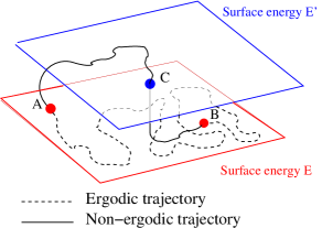
Figure 2: Schematic picture of the type of ergodic dynamics considered in a partial equilibration scenario. Any phase-space points $A,B$ contained in the surface of energy $E$ must be connected by a path lying in that surface (dashed line). Note that other paths (continuous line going through $C$) that we call non-ergodic (as they change the energy of the trajectory) might also exist as the original dynamics of the system coupled to the bath is ergodic.

Eq. (4) states that in an adiabatic regime the energy remains practically constant during timescales of the order of the decorrelation time $\tau_{\rm decorr}(s)$. Therefore, as correlations decay in timescales much shorter than the energy does, the system can explore a large number of configurations within a given region of phase space. In case only spontaneous relaxation takes place, the system is constrained to reach a quasi-stationary state where all configurations lying in a given constant energy surface have the same probability. Equiprobability is guaranteed by the fact that microscopic dynamics over the constant energy surface is ergodic and satisfies detailed balance, i.e. it is reversible over the constant energy surface. The process where a given region of the constant energy surface is sampled according to the microcanonical ensemble (i.e. all configurations lying in that surface have the same probability to be visited) will be termed partial equilibration.

For later purposes we define the complexity ${\cal S}_{E}(A)$ by the relation

$${\cal S}_{E}(A)=\log(\Omega_{E}(A))=\log\Bigl{[}\sum_{{\cal C}}\delta(E-E({\cal C}))\delta(A-A(\cal C))\Bigr{]}$$ (5)

where $\Omega_{E}(A)$ stands for the number of configurations with energy $E$ and observable $A$ . For the total complexity $S(E)$ we have,

$$S(E)=\log(\Omega(E))=\log\Bigl{[}\sum_{{\cal C}}\delta(E-E({\cal C}))\Bigr{]}$$ (6)

where now $\Omega(E)$ is the number of configurations with energy $E$ irrespective of the value of the observable $A$, $\Omega(E)=\int dA\Omega_{E}(A)$. In (5) we use the energy label $E$ as a subindex and not as an additional argument, just to stress its key role in the dynamics compared to that of other observables. Note that we could equally well use the subindex $s$, as for a given age $s$ the average energy of the system is fully determined by the dynamics.

4.2 A fluctuation theorem in the aging state

In a partial equilibration scenario transitions between configurations lying at different constant energy surfaces (i.e. transitions that increase or decrease the energy) are not equiprobable. However, after applying an external perturbation, a shift of energy levels takes place and some configurations, initially belonging to different energy surfaces, may end up into the same one. We show below in Sec. 4.3 how the response of the system to an external perturbation is determined by the density of energy levels just around the reference value $E(s)$. Accordingly, transition rates between configurations having different energies $E,E^{\prime}$, were they equiprobable, are described by the following microcanonical relation,

$$\frac{P(\Delta E)}{P(-\Delta E)}=\frac{\Omega(E^{\prime})}{\Omega(E)}$$ (7)

where $\Delta E=E^{\prime}-E$ is the (intensive) energy difference between both configurations. It is important to point out that $P(\Delta E)$ is not the actual transition rate, but the rate the system would display if transitions between configurations having different energies were equiprobable, a situation that is encountered only after shifting the energy levels (by applying an external perturbation) and redistributing them into a unique energy surface.

Eq. (7) has the form of a FT since it describes the ratio of rates in the forward $E\to E^{\prime}$ and the reverse $E^{\prime}\to E$ directions. Fluctuation theorems, similar to (7), have been derived in other contexts, for instance in systems in steady states [9] or systems arbitrarily perturbed from an initial equilibrium state [10]. From (6) we can write,

$$\frac{P(\Delta E)}{P(-\Delta E)}=\exp\Bigl{[}\Bigl{(}\frac{\partial S(E)}{\partial E}\Bigr{)}\Delta E)\Bigr{]}=\exp\Bigl{[}\frac{\Delta E}{T_{\rm eff}^{\rm FT}(s)}\Bigr{]}$$ (8)

where we have expanded the complexity $S(E)$ and kept only the first term in $\Delta E$ . The factor $T_{\rm eff}^{\rm FT}(s)$ in the exponent in the r.h.s of (11) defines an effective temperature,

$$\frac{1}{T_{\rm eff}^{\rm FT}(s)}=\Bigl{(}\frac{S(E)}{\partial E}\Bigr{)}_{E=E(s)}$$ (9)

where we specifically include the subindex $s$ to denote its time dependence through the value of the energy $E$ at age $s$. The super-index FT indicates that this effective temperature is derived from the fluctuation theorem (7). For a Gaussian $P(\Delta E)$ the value of $T_{\rm eff}^{\rm FT}(s)$ can be shown to be proportional to the width of the exponential tail $\lambda(s)$ as depicted in Fig. 1. This connection has been exploited in [5] as a possible way to estimate the effective temperature from intermittency measurements.

Eqs. (7,8) may look as simple detailed balance but it is not. Detailed balance is a inherent property of the microscopic dynamics. Two are the main differences between (8,9) and microscopic detailed balance. In the former we assumed equiprobability between transitions with identical energies and this is not guaranteed if not in the partial equilibration scenario. Moreover the factor (9) in the exponent of (8) is not the temperature of the bath as implied by detailed balance, but a quantity that is solely determined by the dynamics.

We contend to show that $T_{\rm eff}^{\rm FT}(s)$ as derived from the fluctuation theorem coincides with the effective temperature derived from the FDT relations that link correlations and responses in the aging regime. The origin of this connection has been already mentioned. Eq. (7) links transitions between configurations with different energies. These transitions can be probed only by lifting the energy of the different configurations after applying an external field.

4.3 Microcanonical relations and effective temperatures in the aging state.

Let us consider $A$ to be any observable of the system that can take different values in a given surface of constant energy $E$. The equiprobability assumption implies that the transition rates between configurations with different observable values $A,A^{\prime}$, at a given age $s$ (when the surface explored has energy $E$), satisfy the following relation,

$$\frac{W_{E}(\Delta A)}{W_{E}(-\Delta A)}=\frac{\Omega_{E}(A^{\prime})}{\Omega_{E}(A)}$$ (10)

where $\Delta A=A^{\prime}-A$ and $\Omega_{E}(A)$ was defined in (5). The ratio of rates (10) is therefore age dependent as the value of $E$ changes with the age of the system. Eq. (10) says that the rate for the observable $A$ to change its value in $\Delta A$ within the surface of constant energy $E$, when going from the value $A$ to the value $A^{\prime}$, is proportional to the number of configurations with value $A^{\prime}$ at the energy $E$. Although (10) describes rates there is no explicit reference to any timescale. In fact, we use the term $W$ for these rates (as compared with the term $P(\Delta E)$ used in (7)) to stress the fact that these are rates rather than probabilities (i.e. they have dimensions of a frequency). Note that the difference between using $P$ or $W$ is minor as any timescale drops off when considering the ratio among the forward and reverse rates. Again, as was done for (7), we expand the term in the r.h.s. of (10) around $A^{\prime}=A$ by using  (5) and consider only the first term in the expansion,

$$\frac{W_{E}(\Delta A)}{W_{E}(-\Delta A)}=\exp\Bigl{[}\Bigl{(}\frac{\partial{\cal S}_{E}(A)}{\partial A}\Bigr{)}\Delta A+{\cal O}((\Delta A)^{2})\Bigr{]}$$ (11)

The variation $\Delta A=A^{\prime}-A$ is intensive, therefore all powers of $\Delta A$ enter in (11) even in the thermodynamic limit. However, as we will see later, only the first term is relevant for the emergence of effective temperatures. Here we will not discuss the possible relevance of higher order terms . Relation (11) says that dynamics evolves towards configurations that have a higher value of the complexity ${\cal S}_{E}(A)$, i.e. towards the maximum value $A^{*}(E)$ of ${\cal S}_{E}(A)$,

$$\Bigl{(}\frac{\partial{\cal S}_{E}(A)}{\partial A}\Bigr{)}_{A=A^{*}(E)}=0$$ (12)

As the value of $E$ is time dependent it is also the value of the maximum $A^{*}(E)$. In a partial equilibration scenario, $A$ relaxes (along timescales of order of $\tau_{\rm decorr}(s)$) to the value $A^{*}(E)$ given in (12). This value changes in time as the energy decreases and is slaved to the time evolution of the energy. As the energy decreases much slower than $A$ relaxes to $A^{*}(E)$ (c.f. (4)), reversibility holds in the aging regime,

$$W_{E}(\Delta A)=W_{E}(-\Delta A)~{}~{}~{}~{}.$$ (13)

An interesting and special class of observables are those called neutral where, for large enough times, the value of $A^{*}(E)$ is independent of $E$ (i.e. of the age of the system) $A^{*}(E)=A^{*}$. Therefore the value $A^{*}$ must coincide with the equilibrium value $A^{\rm eq}$ if the system has to equilibrate. Neutral observables have the interesting property that they reach a stationary value exponentially fast and their time evolution is not slaved to that of the energy. The most prominent example of neutral observables is the wave vector density $\rho_{k}(t)$ in supercooled liquids which stays negligible at all times as there is no long range order that develops in the amorphous glass state. The dynamics of a neutral observable is therefore quite easy to visualize. Starting from any initial configuration the dynamics of the system quickly evolves towards $A^{*}$ and stays there forever.

Non-neutral observables are expected to relax fast to their value $A^{*}(E)$ and display an interesting non-monotonic behavior as the value $A^{*}(E)$ changes with the age $s$. For instance, if the system starts far from equilibrium but with a value of $A$ corresponding to the equilibrium value $A^{\rm eq}$, initially the system will depart from this value, and follow the time evolution of $A^{*}(E)$ to eventually come back again to $A^{\rm eq}$ after equilibrating. This effect has been observed in structural glasses where the volume density displays non-monotonic behavior in the glass state and is known as the Kovacs effect .

Figure 3: Time evolution of neutral and non-neutral observables. Explanation is given in the text.

We are now in a position to understand the emergence of effective temperatures as usually derived from fluctuation-dissipation relations. Suppose now that at time $s$ an external field of intensity $h$ coupled to the observable $A$ is applied to the system. In the presence of a field the energy of a configuration ${\cal C}$ is shifted by the Zeeman term,

$$E({\cal C})\to E({\cal C})-hA({\cal C})~{}~{}~{}~{}~{}.$$ (14)

Under the field, the surface of constant energy $E$ does not coincide anymore with that at zero field, meaning that configurations with identical energy at zero field (i.e. lying in a given surface of energy $E$) get shifted by different amounts in a field (i.e. finish into different surfaces with different values of $E$). In particular, for a given value of the energy $E$, from all configurations initially lying in the surface at $h=0$, after switching the field some configurations leave the surface, others come onto the surface, finally others stay there (i.e. those with $A({\cal C})=0$).

According to (14), just after the field has been switched on, configurations with a larger value of $A$ decrease their energy relative to their energy at $h=0$ and configurations with a lower value of $A$ increase their energy. However, the complexity $S(E)$ (6) is a monotonic function of the energy, therefore configurations with higher energy are more numerous than those with lower energy. As a result of the action of the field, the number of configurations $\Omega_{E}^{h}(A)$ with a given value of $A$, that lie inside the surface of constant energy $E$, monotonically increases with $A$,

$$\Omega_{E}^{h}(A)=\int dE^{\prime}\Omega_{E^{\prime}}(A)\delta(E-E^{\prime}+hA)=\Omega_{E+hA}(A)=$$

$$\Omega_{E}(A)\Bigl{[}1+\frac{\partial\log(\Omega_{E}(A))}{\partial E}Ah+{\cal O}(h^{2}))\Bigr{]}=\Omega_{E}(A)\exp\Bigl{[}\Bigl{(}\frac{\partial{\cal S}_{E}(A)}{\partial E}\Bigr{)}Ah+{\cal O}(h^{2})\Bigr{]}~{}~{}~{}.$$ (15)

Using the equivalent of (5), ${\cal S}_{E}^{h}(A)=\log(\Omega_{E}^{h}(A))$, we get,

$${\cal S}_{E}^{h}(A)={\cal S}_{E}(A)+\Bigl{(}\frac{\partial{\cal S}_{E}(A)}{\partial E}\Bigr{)}Ah+{\cal O}(h^{2})={\cal S}_{E}(A)+\beta_{\rm eff}(E,A)Ah+{\cal O}(h^{2})$$ (16)

where we have defined,

$$\beta_{\rm eff}(E,A)=\Bigl{(}\frac{\partial{\cal S}_{E}(A)}{\partial E}\Bigr{)}_{E=E(s),A=A(s)}$$ (17)

As ${\cal S}_{E}(A)$ is a monotonic increasing function of $E$, (15) indicates that relaxation in a field is pushed towards configurations with progressively increasing values of $A$. In a field partial equilibration occurs again in the new surface of energy $E$ as all configurations there contained remain equiprobable. The new  (10) reads,

$$\frac{W_{E}^{h}(\Delta A)}{W_{E}^{h}(-\Delta A)}=\frac{\Omega_{E}^{h}(A^{\prime})}{\Omega_{E}^{h}(A)}=\frac{W_{E}(\Delta A)}{W_{E}(-\Delta A)}\exp(\beta_{\rm eff}(E,A)\Delta A\,h)$$ (18)

where (15,16) have been used. A word of caution in the derivation of  (18) is in place. We have considered $\beta_{\rm eff}(E,A)=\beta_{\rm eff}(E,A^{\prime})$. This is justified as the quantity ${\cal S}_{E}(A)$ entering into the definition (17) is extensive, i.e. proportional to the volume $V$ of the system, while $\Delta A=A^{\prime}-A$ is an intensive quantity. In the large $V$ limit, the partial derivative  (17) is the same whether it is taken at $A$ or $A^{\prime}$ as the difference $\Delta A=A^{\prime}-A$ is intensive so $\beta_{\rm eff}(E,A)-\beta_{\rm eff}(E,A^{\prime})\sim{\cal O}(1/V)$.

Eq. (18) is reminiscent of detailed balance, however the same remark has to be made here as was done in Sec. 4.2. The quantity $\beta_{\rm eff}(E,A)$ is not the temperature of the bath anymore but a time dependent value as $E(s)$ and $A(s)$ change in time. The quantity $\beta_{\rm eff}(E,A)$ defines an effective temperature as obtained from the microcanonical relation (MR)  (18),

$$\frac{1}{T_{\rm eff}^{{\rm MR},A}(s)}=\beta_{\rm eff}(E,A)=\Bigl{(}\frac{\partial{\cal S}_{E}(A)}{\partial E}\Bigr{)}_{E=E(s),A=A(s)}~{}~{}~{}.$$ (19)

As $A(s)=A^{*}(E(s))$ (see (12) and the ensuing discussion) we can replace the complexity ${\cal S}_{E}(A)$ by the total complexity $S(E)$ in the r.h.s of (19). Notably this gives a value of $T_{\rm eff}^{{\rm MR}}(s)$ that is independent on the type of observable so the label $A$ in the l.h.s of (19) drops off,

$$\frac{1}{T_{\rm eff}^{{\rm MR}}(s)}=\beta_{\rm eff}^{{\rm MR}}(s)=\Bigl{(}\frac{\partial{\cal S}_{E}(A))}{\partial E}\Bigr{)}_{E=E(s),A=A(s)}=\Bigl{(}\frac{\partial S(E)}{\partial E}\Bigr{)}_{E=E(s)}~{}~{}~{},$$ (20)

which coincides with the result obtained from the FT (9).

From relation (18) it is now possible to link the autocorrelation and response functions (2) through via the FDR, where the effective temperature (20) appears explicitly,

$$R_{A}(t,s)=\frac{1}{T_{\rm eff}^{{\rm MR}}(s)}\frac{\partial C_{A}(t,s)}{\partial s}\theta(t-s)~{}~{}~{}.$$ (21)

We are not going to show here the details of this derivation but only mention the main steps. The proof follows the scheme of the derivation shown in Section 3 of Ref. [3] for the standard derivation of FDT where (18) here corresponds to (49) there. In [3] it is shown how the response function can be decomposed in two different contributions called $R^{(1)}$ and $R^{(2)}$. In equilibrium, when FDT holds, $R^{(1)}$ vanishes and $R^{(2)}$ gives the equilibrium response. In the partial equilibration scenario, (21) is obtained whenever $R^{(1)}$ vanishes. Close inspection of (53) in [3] shows that this term vanishes only if the perturbing field does not modify, to linear order in $h$, the trapping time distribution measured over transitions starting at the surface of energy $E$. More precisely, consider a sample of all trapping times for configurations of age equal to $s$. As dynamics is stochastic, the same quenching protocol will generate different configurations with values $E,A$ in the vicinity of their dynamical averages $E(s),A(s)$. Let $p_{s}(\tau),p_{s}^{h}(\tau)$ be the trapping time distributions both at zero field and after applying a field $h$ at time $s$ respectively. Eq. (21) holds whenever $p_{s}^{h}(\tau)=p_{s}(\tau)+{\cal O}(h^{2})$ . In other words, up to linear order in $h$ the sole effect of the field is to modify the density of configurations as indicated in (15).

The physical significance of these results can now be appreciated at its full extent. In the simplest partial equilibration scenario the effective temperature derived from the microcanonical relation  (20) is independent on the type of observable and coincides with that obtained from the FT (9) and the FDR (3). For the last equality, the trapping time distribution is required to remain unchanged at linear order with the intensity of the field $h$. In this case,

$$T_{\rm eff}^{{\rm FDR}}(s)=T_{\rm eff}^{\rm FT}(s)=T_{\rm eff}^{{\rm MR}}(s)$$ (22)

This equality is remarkable as it shows that the effective temperature can be directly obtained from the fluctuation theorem (9) without the necessity of introducing a perturbing field and measuring correlations and responses . The first equality in (22) has been numerically verified in a given example of spin-glass model [5]. In what follows we exemplify these results for a simple solvable case.

5 The oscillator model (OM)

Exactly solvable oscillator models (OMs) [8], unrealistic as they look, provide a simple physical basis to describe glassy dynamics. A parallel can be established between oscillator models for glassy dynamics and the original urn models by the Ehrenfest’s. The former can enlighten our comprehension of the essential features of glassy dynamics, in the same way urn models have provided a ground basis to understand key concepts of equilibrium thermodynamics such as the Boltzmann entropy. The OM is an example where the partial equilibration scenario holds for the dynamics at $T=0$. It provides an excellent framework to verify the statements of previous sections.

5.1 Energy relaxation

The OM [8] is described by a set of continuous variables $x_{i}$ and an energy function,

$$E=\frac{K}{2}\sum_{i=1}^{N}x_{i}^{2}$$ (23)

where $K$ is the spring constant and $N$ is the total number of oscillators. Oscillators are non-interacting and therefore the model has trivial static properties, the total energy $E=Nk_{B}T/2$ according to the equipartition law. We consider a cooperative dynamics where oscillators are updated according to the rule $x_{i}\to x_{i}+\frac{r_{i}}{\sqrt{N}}$, the $r_{i}$ being uncorrelated Gaussian variables with $\overline{r_{i}}=0$ and variance $\overline{r_{i}r_{j}}=\Delta^{2}\delta_{ij}$. The updating of all oscillators is carried out in parallel and the moves are accepted according to the Metropolis rule. We will focus our analysis on the dynamics at $T=0$ where only updates that decrease the total energy are accepted. This leads to slow dynamics as most of the proposed moves tend to increase the energy and only few of them are accepted (i.e. the acceptance rate is quickly decreasing with time). Dynamics in the OM is ergodic if confined to a constant energy surface (see Fig. 2). Therefore, dynamics does not become arrested at $T=0$ as no metastable configurations (except the ground state) exist at $T=0$.

Dynamical properties in the OM are derived from the distribution of attempted energy changes $P(\Delta E)$. There are several ways to compute this distribution [15], the simplest one derives from the Gaussian character of such distribution. The change in energy of an elementary move is given by

$$\Delta E=\frac{K}{\sqrt{N}}\sum_{i}\,x_{i}r_{i}+\frac{K}{2N}\sum_{i}r_{i}^{2}.$$ (24)

From the Gaussian character the of $r_{i}$, it follows that $\Delta E$ has a Gaussian distribution whose mean and variance are given by,

$$M_{\Delta E}=\overline{\Delta E}=K\Delta^{2}/2,~{}~{}~{}~{}~{}~{}\sigma_{\Delta E}=\overline{(\Delta E)^{2}}-(\overline{\Delta E})^{2}=2K\Delta^{2}\frac{E}{N}=2K\Delta^{2}e~{}~{}~{}$$ (25)

which yields [8],

$$P(\Delta E)=\bigl{(}4\pi eK\Delta^{2}\bigr{)}^{-\frac{1}{2}}\exp\left[-\frac{(\Delta E-\frac{K\Delta^{2}}{2})^{2}}{4eK\Delta^{2}}\right]$$ (26)

where $e=E/N$ is the energy per oscillator. At $T=0$, the dynamical evolution of the energy $e$ and the acceptance rate $a(e)$ (the fraction of accepted moves) are given by the following closed equations,

$$\frac{\partial e}{\partial t}=\int_{-\infty}^{0}xP(x)\,dx~{}~{}~{}~{}~{};~{}~{}~{}~{}a(e)=\int_{-\infty}^{0}dxP(x)=\frac{1}{2}{\rm Erfc}(\sqrt{\frac{K\Delta^{2}}{16e}})$$ (27)

with ${\rm Erfc}(x)=(2/\sqrt{\pi})\int_{x}^{\infty}du\exp(-u^{2})$ the complementary error function. As the energy $e$ decreases the variance of the distribution (25) decreases. Accordingly, the acceptance rate also decreases. The dynamical evolution of the energy and acceptance can be solved in the long-time limit, $E(t)\sim 1/\log(t),a(t)\sim 1/(t\log(t))$.

5.2 Effective temperature

Correlations and responses have been computed for the magnetization $M=\sum_{i}x_{i}$ [8]. In the rest of the paper we will consider $A=M$ as the observable under quest. $M$ is a neutral observable as can be verified by solving the dynamical equation for the magnetization. It relaxes exponentially fast to zero which is the equilibrium value of the magnetization at all temperatures. The autocorrelation function $C_{M}(t,s)=(1/N)\sum_{i}x_{i}(t)x_{i}(s)$, the corresponding response function $R_{M}(t,s)$ (2) and the susceptibility $\chi_{M}(t,s)=\int_{s}^{t}R_{M}(t,t^{\prime})dt^{\prime}$, do not have stationary part but only aging part and show simple aging with $\tau_{\rm decorr}(s)\propto s$. Correlations and responses define an effective temperature $T_{\rm eff}(t,s)$ through the relation,

$$T_{\rm eff}^{\rm FDR}(t,s)=\frac{\frac{\partial C_{M}(t,s)}{\partial s}}{R_{M}(t,s)}$$ (28)

which is the temperature $T$ of the bath in equilibrium. At $T=0$ the response is finite in the OM due to the shift of energy levels described in Sec. 4.3. A simple expression can be derived in that case,

$$T_{\rm eff}^{\rm FDR}(t,s)\equiv T_{\rm eff}^{\rm FDR}(s)=2e(s)+\frac{1}{f(s)}\frac{\partial e(s)}{\partial s}$$ (29)

where $f(s)$ is a given function [8] which asymptotically decays as $1/s$. Two remarkable facts emerge from (29): 1) $T_{\rm eff}(t,s)$ only depends on the lowest time $s$, therefore characterizes the aging state of the system at time $s$; 2) The second term in the r.h.s of (29) is sub-dominant respect to the first term leading to $T_{\rm eff}(s)\to 2e(s)$, i.e. the equipartition law is asymptotically satisfied in the aging regime.

5.3 The fluctuation theorem

As the energy decays logarithmically and $\tau_{\rm decorr}(s)\propto s$, (4) is satisfied and relaxation is adiabatic. Moreover, dynamics in this model is ergodic if constrained to the constant energy surface. Under these conditions, only spontaneous relaxation occurs (Sec. 3) and partial equilibration holds (Sec. 4.1). We can verify the validity of the FT by substituting (26) in (8),

$$\frac{P(\Delta E)}{P(-\Delta E)}=\exp\Bigl{(}\frac{\Delta E}{T_{\rm eff}^{\rm FT}}\Bigr{)}=\exp\Bigl{(}\frac{\Delta E}{2e}\Bigr{)}$$ (30)

giving $T_{\rm eff}^{\rm FT}=2e$. This result coincides with the asymptotic value $T_{\rm eff}^{\rm FDR}$ previously obtained  (29).

5.4 Trapping time distribution

Here we compute the trapping time distributions without and in a field $p_{s}(\tau),p_{s}^{h}(\tau)$. In the presence of a field the energy of the OM is given by,

$$E=Ne_{T}=\frac{K}{2}\sum_{i=1}^{N}x_{i}^{2}-h\sum_{i=1}^{N}x_{i}=N(e-hm)$$ (31)

where $e,m$ denote $(K/2)\overline{x^{2}}$ and $\overline{x}$ (i.e. the energy and magnetization per oscillator respectively), the total energy per oscillator being $e_{T}=e-hm$. Eq. (31) can be written as $E=\frac{K}{2}\sum_{i=1}^{N}(x_{i}-h/K)^{2}-Nh^{2}/(2K)$. The updating rule for the shifted variables $y_{i}=x_{i}-h/K$ remains unchanged. Consequently, the evolution equation for the quantity $e^{\prime}=(K/2)\overline{y^{2}}=e-hm+h^{2}/(2K)=e_{T}+h^{2}/(2K)$ is identical to that obtained for $e$ at $h=0$. As the time evolution of $e^{\prime}$ does not depend on $h$ this implies that $e_{T}$ gets corrections that are even powers of $h$. In a field, (27) holds by replacing $e$ with $e^{\prime}$. Therefore, the acceptance rate is not modified at linear order in $h$. In general, the trapping time probability distribution is given by $p_{s}^{h}(\tau)=a^{h}(e^{\prime})(1-a^{h}(e^{\prime}))^{\tau-1}$ where $\tau$ is the finite number of Monte Carlo steps (i.e. does not scale with $N$) and $a^{h}(e^{\prime})$ is the acceptance rate in a field. The same expression is valid for $p_{s}(\tau)$ putting $h=0$. This immediately proves that the distribution of trapping times remains unchanged at linear order in $h$. In particular, the average trapping time is finite and given by the inverse of the acceptance rate,

$$\overline{\tau^{h}(e^{\prime})}=\frac{\tau_{0}}{\int_{-\infty}^{0}P_{h}(\Delta E)d(\Delta E)}=\frac{\tau_{0}}{a^{h}(e^{\prime})}$$ (32)

where $\tau_{0}$ is a microscopic time.

5.5 Microcanonical rates for the magnetization

Let us consider the joint probability $P^{h}(\Delta E,\Delta M)$ of having a change in the total energy $\Delta E$ and magnetization $\Delta M$ in the presence of an external field $h$ ($E$ is given in  (31) and includes the Zeeman term). At $T=0$, the probability $a^{h}_{E}$ that an attempted change $\Delta M$ is accepted is given by,

$$W^{h}_{E}(\Delta M)=\frac{1}{\tau_{0}}\int_{-\infty}^{0}P^{h}(\Delta E,\Delta M)d(\Delta E)=\frac{1}{\tau_{0}}P^{0}(\Delta M)\int_{-\infty}^{0}P^{h}_{c}(\Delta E|\Delta M)d(\Delta E)~{}~{}~{}.$$ (33)

where $P^{h}(\Delta E,\Delta M)=P^{h}_{c}(\Delta E|\Delta M)P^{0}(\Delta M)$, the subscript $c$ standing for conditional probability . Again, it is easy to show that these distributions are all Gaussian. Straightforward calculations give,

$$P^{0}(\Delta M)=(2\pi\Delta^{2})^{-\frac{1}{2}}\exp\Bigl{[}-\frac{(\Delta M)^{2}}{2\Delta^{2}}\Bigr{]}$$ (34)

$$P^{h}_{c}(\Delta E|\Delta M)=(2\pi\alpha_{h}^{2})^{-\frac{1}{2}}\exp\Bigl{[}-\frac{(\Delta E-\frac{K\Delta^{2}}{2}-b_{h}\Delta M)^{2}}{2c_{h}^{2}\sigma_{h}^{2}}\Bigr{]}$$ (35)

with the definitions $\alpha_{h}=c_{h}\sigma_{h}$, $b_{h}=g_{h}\sigma_{h}^{2}$, $\sigma_{h}^{2}=2Ke+h^{2}-2Khm$, $c_{h}^{2}=\Delta^{2}(1-\frac{(Km-h)^{2}}{\sigma_{h}^{2}})$, $g_{h}=(Km-h)/(2Ke+h^{2}-2Khm)$. In the linear response regime we obtain, $g_{h}=\frac{m}{2e}+(m^{2}/(2e^{2})-1/(2Ke))h+{\cal O}(h^{2})$, $c_{h}^{2}=c_{0}^{2}(1+mh/e+{\cal O}(h^{2}))$, $c_{0}^{2}=\Delta^{2}(1-m^{2}K/(2e))$, $\sigma_{h}^{2}=2Ke(1-hm/e+{\cal O}(h^{2}))$,$b_{h}=mK-h+{\cal O}(h^{2})$. Inserting (34,35) in (33) gives,

$$W^{h}_{E}(\Delta M)=W_{E}(\Delta M)\exp\Bigl{[}\frac{(\Delta M)h}{4e-2m^{2}K}(1+\frac{2m\Delta M}{\Delta^{2}})\Bigr{]}$$ (36)

$$W_{E}(\Delta M)=\frac{1}{\tau_{0}}\frac{P^{0}(\Delta M)}{2}{\rm Erfc}\Bigl{[}\frac{(k\Delta^{2})/2+b_{0}(\Delta M)}{2^{1/2}\alpha_{0}}\Bigr{]}$$ (37)

where $P^{0}(\Delta M)$ is given by (34). As $m$ is a neutral observable that relaxes fast to $0$ we can replace $m=0$ everywhere in all previous expressions. Up to linear order in $h$ the rates $W_{E}^{h}$ are given by,

$$W^{h}_{E}(\Delta M)=W_{E}(\Delta M)\exp\Bigl{(}\frac{\Delta Mh}{4e}\Bigr{)}~{}~{}~{}~{}~{}~{};~{}~{}~{}~{}~{}~{}~{}~{}W_{E}(\Delta M)=P^{0}(\Delta M)a(e)$$ (38)

where $a(e)$ is given in (27). We remark the following results: 1) the perturbed rates are multiplicative , 2) (13) holds as $W_{E}(\Delta M)=W_{E}(-\Delta M)$ and 3) relation (18) is satisfied as well,

$$\frac{W^{h}_{E}(\Delta M)}{W^{h}_{E}(-\Delta M)}=\frac{W_{E}(\Delta M)}{W_{E}(-\Delta M)}\exp\Bigl{[}\frac{(\Delta M)h}{2T_{\rm eff}^{\rm MR}(e)}\Bigr{]}$$ (39)

so the effective temperature here obtained $T_{\rm eff}^{\rm MR}(e)=2e$ again coincides with that derived from the FDR (29) and the FT (30).

6 Conclusions

A statistical interpretation of a non-equilibrium or effective temperature in aging systems, rather than a thermometric one, might be possible. Recent numerical simulations of a disordered model [5] have shown that the effective temperature, as measured from FDT violations, originate from the existence of a spontaneous relaxational process describing heat exchange low-frequency events. Superimposed to it there is a stimulated process that is characterized by the temperature of the bath and responsible of most of the heat exchange observable events between system and bath. Although the timescale of the spontaneous process is related to the temperature of the bath, its statistical description (e.g. the specific form of the corresponding FT) is related to other properties of the aging state such as the energy content. The concurrence of these two processes in the overall relaxation is related to the intermittent phenomenon recently observed in various experiments [6, 7]. Moreover, the width of the exponential tail associated to the spontaneous process is predicted to be proportional to the effective temperature.

We have investigated a partial equilibration scenario where only the spontaneous process occurs (the temperature of the bath is set to zero) and dynamics is ergodic when constrained to a given energy surface. In this case three effective temperatures can be defined: a) from the fluctuation-dissipation ratio (3); b) from the fluctuation theorem for the statistical description of the spontaneous component (7); c) from microcanonical relations relating observable changes (20). All three are shown to be identical (22). Explicit calculations in the OM demonstrate the validity of these statements.

Several open questions and directions of research along the present ideas appear worthwhile. It would be useful to go beyond the qualitative level of demonstrations in the present paper over more founded mathematical proofs of all these results. Attempts trying to establish the origin of effective temperatures using master equation formalisms have already appeared in the literature [13, 18] and we foresee more work in the near future. We should also mention the close similarity between the present approach and that by Edwards for granular matter [19]. Would be very interesting to investigate other classes of models with simple equilibrium properties, such as kinetically constrained models [20], where the existence of non-trivial effective temperatures is still under debate. In these models it is possible to identify correlated motion of particles [21] that underpin a spatially heterogeneous dynamics [22]. Another category of interesting problems to explore are systems in steady states where FDT violations have been studied [23] and where non-Gaussian effects, similar to those described here, have been identified as well [24].

References

- [1] J. Casas-Vazquez and D. Jou, Rep. Prog. Phys. 66, 1937 (2003).
- [2] L. F. Cugliandolo, J. Kurchan and L. Peliti, Phys. Rev. E 55, 3898 (1997).
- [3] A. Crisanti and F. Ritort, J. Phys. A (Math. Gen.), 36, R181-R290 (2003).
- [4] L. F. Cugliandolo, D. S. Dean and J. Kurchan, Phys. Rev. Lett 79, 2168 (1997).
- [5] A. Crisanti and F. Ritort, Preprint cond-mat/0307554
- [6] L. Buisson, L. Bellon and S. Ciliberto, J. Phys. C (Cond. Matt.) 15, S1163 (2003)
- [7] L. Cipelletti et al., J. Phys. C (Cond. Matt.) 15, S257 (2003)
- [8] L. L. Bonilla, F. G. Padilla and F. Ritort, Physica A, 250, 315 (1998).
- [9] D. Evans and Searles, Adv. Phys. 51, 1529 (2002).
- [10] G. E. Crooks, J. Stat. Phys. 90, 1481 (1998).
- [11] E. M. Bertin, J. P. Bouchaud, J. M. Drouffe and C. Godreche, Preprint cond-mat/0306089
- [12] A. Buhot, Preprint cond-mat/0310311
- [13] C. Chatelain, J. Phys. A (Math. Gen.), 36, 10739 (2003)
- [14] F. Ricci-Tersenghi, Preprint cond-mat/0307565
- [15] A detailed exposition can be found in Sec. 6.5.1 of [3].
- [16] F. Ritort, J. Phys. A (Math. Gen.), 36, 10791 (2003)
- [17] P. Sollich, J. Phys. A (Math. Gen.), 36, 10807 (2003)
- [18] G. Diezemann, Preprint cond-mat/0309105
- [19] S. F. Edwards, Physica A, 157, 1080 (1898).
- [20] F. Ritort and P. Sollich, Adv. Phys. 52, 219 (2003)
- [21] J. P. Garrahan and D. Chandler, Proc. Nat. Acad. Sci. 100, 9710 (2003)
- [22] L. Berthier and J. P. Garrahan, Preprint condmat/0306469
- [23] I. Santamaría-Holek, D. Reguera and J. M. Rubí, Phys. Rev. E 63, 051106 (2001)
- [24] R. van Zon and E. G. D. Cohen, Preprint cond-mat/0310265