Penetration depth anisotropy in two-band superconductors

V. G. Kogan, N. V. Zhelezina Ames Laboratory - DOE and Department of Physics, Iowa State University, Ames, IA 50011
(July, 2003; )
Abstract

The anisotropy of the London penetration depth is evaluated for two-band superconductors with arbitrary inter- and intra-band scattering times. If one of the bands is clean and the other is dirty in the absence of inter-band scattering, the anisotropy is dominated by the Fermi surface of the clean band and is weakly temperature dependent. The inter-band scattering also suppress the temperature dependence of the anisotropy.

pacs:
74.70.Ad, 74.25.Nf, 74.60.-w

The two-gap superconductivity of MgB2 is established experimentally Bouquet ; Szabo ; Giubileo ; Junod ; Schmidt and by solving the Eliashberg equations for the gap distribution on the Fermi surface.Choi ; Mazin According to the latter, the gap on the four Fermi surface sheets of this material has two sharp maxima: $\Delta_{1}\approx 1.7\,$meV at the two $\pi$-bands and $\Delta_{2}\approx 7\,$meV at the two $\sigma$-bands. Within each of these groups, the spread of the gap values is small.

A number of physical properties of MgB2 were reasonably well described within a model with two constant gaps on two separate Fermi sheets. Still, the data on anisotropy of the magnetic field penetration depth $\lambda$ are controversial. The anisotropy parameter $\gamma_{\lambda}=\lambda_{c}/\lambda_{a}$ has been calculated within the weak-coupling clean-limit model and shown to increase from about 1.1 at $T=0$ to $\approx 2.6$ at $T_{c}$. Kogan Similar prediction has been made within Eliashberg formalism. Golubov Qualitatively, the predictions were confirmed in STM, STM ; Morten small angle neutron scattering, Cubitt and magnetization experiments. Lyard However, other groups recorded different behavior. Jap-torque ; Angst ; Caplin Given variety of samples used, it seems imperative to consider effects of scattering upon $\gamma_{\lambda}$, a non-trivial problem given different roles of the intra- and inter-band scattering in two-band materials.

In the following, we reiterate that in the presence of inter-band scattering, the energy gap in the quasiparticle excitation spectrum as revealed by the density of states (DOS) differs from both $\Delta_{1}$ and $\Delta_{2}$, Mosk1 ; Schop the situation reminiscent of the Abrikosov-Gor’kov pair breaking. AG For this reason, we use the term “order parameter” for $\Delta$’s. We stress that all thermodynamic properties depend on the actual DOS and are affected by the inter-band scattering. Then, we show that $\gamma_{\lambda}=\lambda_{c}/\lambda_{ab}$ depends on both inter- and intra-band scattering.

Our approach is based on the quasiclassical version of the BCS theory for a general anisotropic Fermi surface and for an arbitrary anisotropic order parameter $\Delta({\bm{k}})$. Eil In the absence of currents and fields we have for the Eilenberger Green’s functions $f({\bm{k}},\omega)$ and $g({\bm{k}},\omega)$:

$$0=2\Delta g-2\omega f+I\,,\qquad 1=g^{2}+f^{2}\,.$$ (1)

Here the scattering term $I$ is given by the integral over the full Fermi surface:

$$I({\bm{k}})=\int d^{2}{\bm{q}}\,\rho({\bm{q}})\,W({\bm{k}},{\bm{q}})\,[g({\bm{k}})f({\bm{q}})-f({\bm{k}})g({\bm{q}})]$$ (2)

with $W({\bm{k}},{\bm{q}})$ being the scattering probability from ${\bm{q}}$ to ${\bm{k}}$ at the Fermi surface. The Matsubara frequencies are $\omega=\pi T(2n+1)$ with an integer $n$ ($\hbar=1$). The local DOS $\rho({\bm{q}})$ is normalized: $\int d^{2}{\bm{q}}\,\rho({\bm{q}})=1$.

This system (1)-(2) should be complemented with an equation for $\Delta({\bm{k}})$. We will not use it here, rather taking $\Delta({\bm{k}})$ as a given. This simplifies the problem greatly because solving for $\Delta({\bm{k}})$ usually involves a number of assumptions which are difficult to control.

We use the approximation of the scattering time $\tau$:

$$\int d^{2}{\bm{q}}\,\rho({\bm{q}})\,W({\bm{k}},{\bm{q}})\,f({\bm{q}})=\langle f\rangle/\tau\,;$$ (3)

$\langle...\rangle$ stands for the average over the Fermi surface. Clearly, the approximation amounts to the scattering probability $W=1/\tau$ being constant for any ${\bm{k}}$ and ${\bm{q}}$.

For two well-separated Fermi surface sheets, the probabilities of intra-band scatterings may differ from each other and from processes involving ${\bm{k}}$ and ${\bm{q}}$ from different bands. The effects of the inter- and intra-band scattering upon various properties of the system are different, e.g., the intra-band scattering does not affect $T_{c}$, whereas the inter-band does. Therefore, Eq. (3) is replaced by

$$\int d^{2}{\bm{q}_{\alpha}}\,\rho({\bm{q}_{\alpha}})\,W({\bm{k}_{\beta}},{\bm{q}_{\alpha}})\,f({\bm{q}_{\alpha}})=\langle f\rangle_{\alpha}/\tau_{\beta\alpha}\,.$$ (4)

Here $\alpha,\beta=1,2$ are band indices and $\langle...\rangle_{\alpha}$ denotes averaging only over the $\alpha$-band.

We now assume the order parameters $\Delta({\bm{k}}_{\alpha})$ taking constant values $\Delta_{1}$ and $\Delta_{2}$ at each of the two bands. Writing Eq. (1) for ${\bm{k}}$ in the first band, we have:

$\displaystyle 0$ $\displaystyle=2\Delta_{1}g_{1}-2\omega f_{1}$ (5)
$\displaystyle+$ $\displaystyle\frac{1}{\tau_{11}}[g_{1}\langle f\rangle_{1}-f_{1}\langle g\rangle_{1}]+\frac{1}{\tau_{12}}[g_{1}\langle f\rangle_{2}-f_{1}\langle g\rangle_{2}]\,.$

For a uniform sample in zero field and with ${\bm{k}}$ independent $\Delta$’s in each band, the functions $f,g$ are ${\bm{k}}$ independent: $\langle f\rangle_{\alpha}=f_{\alpha}$ and $\langle g\rangle_{\alpha}=g_{\alpha}$. Then, we have:

$\displaystyle 0=\Delta_{1}g_{1}-\omega f_{1}+[g_{1}f_{2}-f_{1}g_{2}]/2\tau_{12}\,.$ (6)

The equation for the second band differs from this by replacement $1\leftrightarrow 2$. The fact that $\tau_{11}$ and $\tau_{22}$ do not enter the system (6) is similar to the case of one-band isotropic material for which non-magnetic scattering has no effect upon $T_{c}$ (the Anderson theorem). It is the inter-band scattering that makes the difference in the two-gap case, the fact stressed already in early work. Mosk1 ; Schop

Two equations (6) are complemented with normalizations $g_{\alpha}^{2}+f_{\alpha}^{2}=1$ to form a sufficient set. Following Ref. AG, , we introduce variables $u_{\alpha}=g_{\alpha}/f_{\alpha}$ and obtain after simple algebra: Sung ; Mosk1 ; Schop

$\displaystyle\frac{\omega}{\Delta_{1}}=u_{1}+\zeta_{1}\frac{u_{1}-u_{2}}{\sqrt{u_{2}^{2}+1}}\,,\qquad\zeta_{1}=\frac{1}{2\tau_{12}\Delta_{1}}\,;$
$\displaystyle\frac{\omega}{\Delta_{2}}=u_{2}+\zeta_{2}\frac{u_{2}-u_{1}}{\sqrt{u_{1}^{2}+1}}\,,\qquad\zeta_{2}=\frac{1}{2\tau_{21}\Delta_{2}}\,.$ (7)

The Eilenberger functions in terms of variables $u$ read:

$$f=1/\sqrt{1+u^{2}}\,,\qquad g=u/\sqrt{1+u^{2}}\,.$$ (8)

In general, the system (7) can be solved only numerically. However, near $T_{c}$, $u=g/f\gg 1$ and one obtains:

$\displaystyle u_{1}=\frac{\omega}{\Delta_{1}}\,\frac{\omega+\zeta_{1}\Delta_{1}+\zeta_{2}\Delta_{2}}{\omega+(\zeta_{1}+\zeta_{2})\Delta_{2}}\,;$ (9)

$u_{2}$ is obtained by $1\leftrightarrow 2$. Clearly, $u_{\alpha}=\omega/\Delta_{\alpha}$ in the absence of inter-band scattering. For $\zeta\gg 1$, we have:

$$u_{1}\approx u_{2}\approx\frac{\omega}{\epsilon^{*}}\,,\quad\epsilon^{*}=\frac{(\zeta_{1}+\zeta_{2})\Delta_{1}\Delta_{2}}{\zeta_{1}\Delta_{1}+\zeta_{2}\Delta_{2}}\,.$$ (10)

Moreover, if the inter-band scattering is strong, Eq. (10) holds at any $T$. To see this, look for solutions of Eqs. (7) in the form

$$u_{\alpha}=\frac{\omega}{\epsilon^{*}}+v_{\alpha}\,,\qquad\alpha=1,2\,\,,$$ (11)

where $v_{\alpha}$ are small corrections. Substitute these in Eqs. (7) and keep only linear terms in $v$ to obtain

$\displaystyle v_{1}$ $\displaystyle=$ $\displaystyle\frac{g^{*}(\epsilon^{*}-\Delta_{1})}{\Delta_{1}[1+g^{*}(\zeta_{1}+\zeta_{2})]}$ (12)
$\displaystyle+$ $\displaystyle\frac{\epsilon^{*}(\zeta_{1}\Delta_{1}+\zeta_{2}\Delta_{2})-\Delta_{1}\Delta_{2}(\zeta_{1}+\zeta_{2})}{\Delta_{1}\Delta_{2}[1+g^{*}(\zeta_{1}+\zeta_{2})]}\,,$

where $g^{*}=\omega/\sqrt{\omega^{2}+\epsilon^{*2}}$. For $\zeta_{\alpha}\to\infty$, $v_{1}$ remains small only if $\epsilon^{*}$ is given by expression (10).

The DOS for two-band materials is $N(\epsilon)=N(0)\,{\rm Re}(\nu_{1}\,g_{1}+\nu_{2}\,g_{2})_{\omega\to i\epsilon}$; $\nu_{\alpha}$ are fractions of the total DOS $N(0)$ at the two pieces of the Fermi surface. For strong inter-band scattering, this gives in the lowest approximation

$$N(\epsilon)=N(0)\,\frac{\epsilon^{*}}{\sqrt{\epsilon^{2}-\epsilon^{*2}}};$$ (13)

i.e., $\epsilon^{*}$ is the common for both bands energy gap.

It does not seem possible to provide a general expression for $\epsilon^{*}$ in terms of $\Delta_{\alpha}$ and an arbitrary inter-band scattering strength. Still, in principle, we can evaluate any thermodynamic property of a two-band material knowing the solutions $u$ of the system (7) and the gap $\epsilon^{*}$.

If the ground state functions (which we call now $f^{(0)}$, $g^{(0)}$) are known, one can study perturbations of the uniform state such as penetration of a weak magnetic field, i.e., the problem of the London penetration depth. The perturbations, $f^{(1)},\,\,g^{(1)}$, should be found from the full Eilenberger equations; Eil we have for the first band:

$\displaystyle{\bm{v}}{\bm{\Pi}}f_{1}=2\Delta_{1}g_{1}-2\omega f_{1}+\frac{1}{\tau_{11}}[g_{1}\langle f\rangle_{1}-f_{1}\langle g\rangle_{1}]$
$\displaystyle+\frac{1}{\tau_{12}}[g_{1}\langle f\rangle_{2}-f_{1}\langle g\rangle_{2}]\,,$ (14)

Here, ${\bm{v}}$ is the Fermi velocity, ${\bm{\Pi}}=\nabla+2\pi i{\bm{A}}/\phi_{0}$. The second equation is obtained by $1\leftrightarrow 2$. Two equations for the “anomalous” functions $f^{+}$ are obtained from these by complex conjugation and by ${\bm{v}}\to-{\bm{v}}$. Eil The normalizations $g_{\alpha}^{2}+f_{\alpha}f_{\alpha}^{+}=1$ complete the system.

We look for solutions in the form

$\displaystyle f_{\alpha}$ $\displaystyle=$ $\displaystyle(f_{\alpha}^{(0)}+f_{\alpha}^{(1)})\,e^{i\theta({\bm{r}})},\quad f_{\alpha}^{+}=(f_{\alpha}^{(0)}+f_{\alpha}^{(1)+})e^{-i\theta({\bm{r}})}\,,$
$\displaystyle g_{\alpha}$ $\displaystyle=$ $\displaystyle g_{\alpha}^{(0)}+g_{\alpha}^{(1)}\,,\qquad\alpha=1,2\,.$ (15)

where $f_{\alpha}^{(0)}$ and $g_{\alpha}^{(0)}$ can be expressed in terms of $u$’s obtained solving the system (7). The form (15) takes into account that in the London approximation only the overall phase depends on coordinates. We obtain for the corrections after some algebra:

$\displaystyle g_{1}^{(1)}\Delta_{1}^{\prime}-f_{1}^{(1)}\omega^{\prime}_{1}=if_{1}^{(0)}{\bm{v}}{\bm{P}}/2\,,$
$\displaystyle g_{1}^{(1)}\Delta_{1}^{\prime}-f_{1}^{(1)+}\omega^{\prime}_{1}=if_{1}^{(0)}{\bm{v}}{\bm{P}}/2\,,$ (16)
$\displaystyle 2g_{1}^{(0)}g_{1}^{(1)}+f_{1}^{(0)}(f_{1}^{(1)}+f_{1}^{(1)+})=0\,,$

where ${\bm{P}}=\nabla\theta+2\pi{\bm{A}}/\phi_{0}$ and

$\displaystyle\Delta_{1}^{\prime}$ $\displaystyle=$ $\displaystyle\Delta_{1}+f_{1}^{(0)}/2\tau_{11}+f_{2}^{(0)}/2\tau_{12}\,,$ (17)
$\displaystyle\omega^{\prime}_{1}$ $\displaystyle=$ $\displaystyle\omega+g_{1}^{(0)}/2\tau_{11}+g_{2}^{(0)}/2\tau_{12}\,.$ (18)

The equations for the second band (decoupled from the first) are obtained by $1\leftrightarrow 2$.

To evaluate the penetration depth we turn to the Eilenberger expression for the current density, Eil

$${\bm{j}}=-4\pi|e|N(0)T\,\,{\rm Im}\sum_{\omega>0}\langle{\bm{v}}g\rangle\,,$$ (19)

and compare it with the London relation

$$\frac{4\pi}{c}j_{i}=-(\lambda^{2})_{ik}^{-1}\left(\frac{\phi_{0}}{2\pi}\nabla\theta+{\bm{A}}\right)_{k}\,.$$ (20)

Here, $(\lambda^{2})_{ik}^{-1}$ is the tensor of the inverse squared penetration depth (proportional to the superfluid density tensor); summation over $k$ is implied. We now find $g_{1}^{(1)}$ from the system (16):

$$g_{1}^{(1)}=\frac{if_{1}^{(0)2}\,{\bm{v}}{\bm{P}}}{2(\Delta_{1}^{\prime}f_{1}^{(0)}+\omega^{\prime}_{1}g_{1}^{(0)})}=i\,\frac{f_{1}^{(0)2}g_{1}^{(0)}}{2\omega^{\prime}_{1}}\,{\bm{v}}{\bm{P}}\,;$$ (21)

$g_{2}^{(1)}$ is obtained by replacement $1\leftrightarrow 2$. Substituting $g_{\alpha}^{(1)}$ in Eq. (19) and comparing with Eq. (20) we obtain:

$\displaystyle(\lambda^{2})_{ik}^{-1}=\frac{16\pi^{2}e^{2}N(0)T}{c^{2}}\sum_{\alpha,\omega}\nu_{\alpha}\langle v_{i}v_{k}\rangle_{\alpha}\frac{f_{\alpha}^{2}g_{\alpha}}{\omega^{\prime}_{\alpha}}\,.$ (22)

Only the unperturbed functions $f,g$ enter the penetration depth; for brevity we dropped the superscript $(0)$. Equation (22) is our main result. Thus, to evaluate the penetration depth for given order parameters $\Delta_{\alpha}$ in the presence of scattering, one has to solve the system (7) for $u_{\alpha}(\omega)$, then to substitute the equilibrium functions $f_{\alpha},\,\,g_{\alpha}$ (given in (8)) in Eq. (22) to sum up over $\omega$.

The band calculations Bel yield for MgB2 the following averages: $\langle v_{a}^{2}\rangle_{1}=33.2$, $\langle v_{c}^{2}\rangle_{1}=42.2$, $\langle v_{a}^{2}\rangle_{2}=23$, and $\langle v_{c}^{2}\rangle_{2}=0.5\times 10^{14}\,$cm2/s2. Tensors $\langle v_{i}v_{k}\rangle_{1}$ and $\langle v_{i}v_{k}\rangle_{2}$ have opposite anisotropies:

$$\frac{\langle v_{a}^{2}\rangle_{1}}{\langle v_{c}^{2}\rangle_{1}}\approx 0.79\,,\quad\frac{\langle v_{a}^{2}\rangle_{2}}{\langle v_{c}^{2}\rangle_{2}}\approx 46.\,,$$ (23)

whereas averaging over the whole Fermi surface yields a nearly isotropic result: $\langle v_{a}^{2}\rangle/\langle v_{c}^{2}\rangle\approx 1.2\,$.

In the clean limit (all ταβsubscript𝜏𝛼𝛽\tau_{\alpha\beta}\to\infty) ω=ωsuperscript𝜔𝜔\omega^{\prime}=\omega and Δα=ΔαsubscriptsuperscriptΔ𝛼subscriptΔ𝛼\Delta^{\prime}_{\alpha}=\Delta_{\alpha}. Besides, uα=ω/Δαsubscript𝑢𝛼𝜔subscriptΔ𝛼u_{\alpha}=\omega/\Delta_{\alpha} and fα2gα/ωα=Δα2/(ω2+Δα2)3/2superscriptsubscript𝑓𝛼2subscript𝑔𝛼subscriptsuperscript𝜔𝛼superscriptsubscriptΔ𝛼2superscriptsuperscript𝜔2superscriptsubscriptΔ𝛼232f_{\alpha}^{2}g_{\alpha}/\omega^{\prime}_{\alpha}=\Delta_{\alpha}^{2}/(\omega^{2}+\Delta_{\alpha}^{2})^{3/2}. Expression (22) reduces to the result given in Ref. Kogan, . For MgB2, it gives nearly isotropic penetration depth at low temperatures: at T=0𝑇0T=0 the sums over ω𝜔\omega in Eq. (22) are the same; this gives γλ(0)=λcc/λaa=va2/vc21.1subscript𝛾𝜆0subscript𝜆𝑐𝑐subscript𝜆𝑎𝑎delimited-⟨⟩superscriptsubscript𝑣𝑎2delimited-⟨⟩superscriptsubscript𝑣𝑐21.1\gamma_{\lambda}(0)=\lambda_{cc}/\lambda_{aa}=\sqrt{\langle v_{a}^{2}\rangle/\langle v_{c}^{2}\rangle}\approx 1.1. Near Tcsubscript𝑇𝑐T_{c}, the sums are Δα2proportional-toabsentsuperscriptsubscriptΔ𝛼2\propto\Delta_{\alpha}^{2}, and the contribution of the strongly anisotropic σ𝜎\sigma-
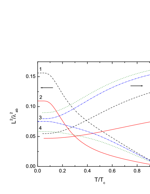
band with the large gap dominates; this gives γλ(Tc)2.6subscript𝛾𝜆subscript𝑇𝑐2.6\gamma_{\lambda}(T_{c})\approx 2.6\,. The curve 1 in Fig. 1 shows γλ(T)subscript𝛾𝜆𝑇\gamma_{\lambda}(T) for this case.

Zero inter-band scattering ($\tau_{12}=\tau_{21}=\infty$). If only the intra-band scattering is present, the functions $f,g$ are the same as in the clean limit. We readily obtain:

$$\frac{f_{\alpha}^{2}g_{\alpha}}{\omega^{\prime}_{\alpha}}=\frac{\Delta_{\alpha}^{2}}{\beta_{\alpha}^{2}(\beta_{\alpha}+1/2\tau_{\alpha\alpha})}\,,$$ (24)

with $\beta_{\alpha}^{2}=\omega^{2}+\Delta_{\alpha}^{2}$. This expression appears in the standard penetration depth calculations, see e.g. Ref. AGD, . For known $\Delta_{\alpha}(T)$, the sums in Eq. (22) can be evaluated numerically; however, for $T\to 0,\,\,T_{c}\,$, and in the dirty limit they can be done analytically.

At $T=0$, the sums are replaced with integrals according to $2\pi T\sum_{\omega}=\int_{0}^{\infty}d\omega$. Denoting ${\cal I}(T)=2\pi T\sum_{\omega}\Delta^{2}/\beta^{2}(\beta+1/2\tau)$ we obtain ${\cal I}(0)=1$ for $\tau\to\infty$ and ${\cal I}(0)=\pi\tau\Delta$ for $\tau\Delta\ll 1$.

Near $T_{c}$, $g\,$ $\to$ $1$ and we have for clean bands $\sum_{\omega}f^{2}/\omega^{\prime}=7\zeta(3)\Delta^{2}/8\pi^{3}T_{c}^{3}$, whereas for dirty bands it is $\tau\Delta^{2}/4T_{c}^{2}$.

Different impurities introduced to MgB2 may affect differently the scattering within the bands. Maz1 ; selective_scattering It is of interest to see how the anisotropy of $\lambda$ is affected by differences in scattering times $\tau_{11}$ and $\tau_{22}$. We first look at two limiting situations when one of the bands is clean while the other is dirty. If the first ($\pi$) band is clean and the second ($\sigma$) is a dirty extreme ($\tau_{22}\Delta_{2}\to 0$), one can disregard the contribution of the dirty band to obtain for both $T=0$ and $T=T_{c}$:

$$\gamma_{\lambda}(0)=\gamma_{\lambda}(T_{c})\approx\sqrt{\frac{\langle v_{a}^{2}\rangle_{1}}{\langle v_{c}^{2}\rangle_{1}}}\approx 0.89\,.$$ (25)

If the ($\pi$) band is dirty and the ($\sigma$) is clean, we have

$$\gamma_{\lambda}(0)=\gamma_{\lambda}(T_{c})\approx\sqrt{\frac{\langle v_{a}^{2}\rangle_{2}}{\langle v_{c}^{2}\rangle_{2}}}\approx 6.8\,.$$ (26)

These two numbers constitute the minimum and maximum possible values for $\lambda$-anisotropy of MgB2. Thus, when one of the bands is clean and the other is dirty we expect a weakly $T$ dependent $\gamma_{\lambda}$, the value of which is determined by the clean band.

If the intra-band scattering is strong in both bands ($\tau_{11}\Delta_{1}\sim\tau_{22}\Delta_{2}\ll 1$, $\tau_{12}=\infty$), the bands contribute to the superfluid density tensor $(\lambda^{2})_{ik}^{-1}$ as two independent dirty superconductors. To see this, we note that $\omega_{1}^{\prime}\approx g_{1}/2\tau_{11}$ and the sums over $\omega$ in Eq, (22) can be evaluated exactly:

$$\sum_{\omega}\frac{f_{1}^{2}g_{1}}{\omega^{\prime}_{1}}=\sum_{\omega}\frac{2\tau_{11}\Delta_{1}^{2}}{\omega^{2}+\Delta_{1}^{2}}=\frac{\tau_{11}\Delta_{1}}{2T}\tanh\frac{\Delta_{1}}{2T}\,.$$ (27)

Then, we arrive at the result obtained by Gurevich with the help of the dirty limit Usadel equations: Sasha

$$(\lambda^{2})_{ik}^{-1}=\frac{4\pi^{2}}{c^{2}\hbar}\sum_{\alpha}\sigma_{ik}^{(\alpha)}\Delta_{\alpha}\tanh\frac{\Delta_{\alpha}}{2T}$$ (28)

where the anisotropic conductivities of the two bands $\sigma_{ik}^{(\alpha)}=2e^{2}\langle v_{i}v_{k}\rangle_{\alpha}\tau_{\alpha\alpha}\nu_{\alpha}N(0)$ are introduced (we write here $\hbar$ explicitly to avoid confusion in dimensions). This yields:

$$\gamma_{\lambda}^{2}(0)=\frac{\sigma_{aa}^{(1)}\Delta_{1}+\sigma_{aa}^{(2)}\Delta_{2}}{\sigma_{cc}^{(1)}\Delta_{1}+\sigma_{cc}^{(2)}\Delta_{2}}\,\,,$$ (29)
$$\gamma_{\lambda}^{2}(T_{c})=\frac{\sigma_{aa}^{(1)}\Delta_{1}^{2}+\sigma_{aa}^{(2)}\Delta_{2}^{2}}{\sigma_{cc}^{(1)}\Delta_{1}^{2}+\sigma_{cc}^{(2)}\Delta_{2}^{2}}\,\,.$$ (30)

Finally, we discuss the possibility of a strong inter-band scattering. As was shown above, in this case $u=\omega/\epsilon^{*}+{\cal O}(1/\zeta)$ in both bands, see Eqs. (11) and (12). Then, the Eilenberger functions are also the same in the two bands: $f=\epsilon^{*}/\sqrt{\omega^{2}+\epsilon^{*2}}$, $g=\omega/\sqrt{\omega^{2}+\epsilon^{*2}}$. Evaluation of the sums over $\omega$ in Eq. (22) is now simple:

$\displaystyle(\lambda^{2})_{ik}^{-1}=\frac{8\pi^{2}e^{2}N(0)}{c^{2}}\,\epsilon^{*}\tanh\frac{\epsilon^{*}}{2T}\sum_{\alpha}\nu_{\alpha}\langle v_{i}v_{k}\rangle_{\alpha}\tau_{\alpha}$ (31)

where $\epsilon^{*}(T)$ is given in Eq. (10) and

$$\tau_{1}=\frac{\tau_{11}\tau_{12}}{\tau_{11}+\tau_{12}}\,,\quad\tau_{2}=\frac{\tau_{22}\tau_{21}}{\tau_{22}+\tau_{21}}\,.$$ (32)

Thus, all components of $(\lambda^{2})_{ik}$ have the same $T$ dependence and the anisotropy parameter is $T$ independent:

$$\gamma_{\lambda}^{2}=\frac{\nu_{1}\langle v_{a}^{2}\rangle_{1}\tau_{1}+\nu_{2}\langle v_{a}^{2}\rangle_{2}\tau_{2}}{\nu_{1}\langle v_{c}^{2}\rangle_{1}\tau_{1}+\nu_{2}\langle v_{c}^{2}\rangle_{2}\tau_{2}}\,.$$ (33)
Refer to caption
Figure 1: The anisotropy $\gamma_{\lambda}=\lambda^{2}_{c}\lambda^{2}_{ab}$ and the inverse square of the penetration depth $L^{2}/\lambda^{2}_{ab}$ versus $T/T_{c}$; $L^{2}=16\pi^{2}e^{2}N(0)\langle v_{a}^{2}\rangle/c^{2}$. The curves labelled 1 is the clean limit, all $1/\tau$ are zero. The curves labelled 2 and 3 are calculated for a weak inter-band scattering: $\tau_{12}\Delta_{1}(0)=500$, $\tau_{21}\Delta_{2}(0)=2000$ ($\hbar=1$); the curve 2 is for a clean $\pi$-band, $\tau_{11}\Delta_{1}(0)=10$, and a dirty $\sigma$, $\tau_{22}\Delta_{2}(0)=0.1$; the curve 3 is for a dirty $\pi$ and clean $\sigma$: $\tau_{11}\Delta_{1}(0)=0.1$, $\tau_{22}\Delta_{2}(0)=10$. Curves 4 are for the intermediate inter-band scattering strength $\tau_{12}\Delta_{1}(0)=5$, $\tau_{21}\Delta_{2}(0)=20$, and $\tau_{11}\Delta_{1}(0)=0.05$, $\tau_{21}\Delta_{2}(0)=2$.

If all $\tau$’s are the same, we have:

$$\gamma_{\lambda}^{2}=\langle v_{a}^{2}\rangle\big{/}\langle v_{c}^{2}\rangle\,.$$ (34)

For $T\to T_{c}$, this result was obtained in Ref. Kogan, ; we now see that it holds at any temperature.

To recover the behavior of $\gamma_{\lambda}(T)$ between 00 and $T_{c}$ one needs explicit dependencies $\Delta(T)$. Qualitatively, this behavior can be studied assuming $\Delta_{\alpha}(T)\approx\Delta_{\alpha}(0)(1-t^{2})$ with, e.g., $\Delta_{2}(0)=4\Delta_{1}(0)=2T_{c}$. Figure 1 shows results of numerical evaluation of $\gamma_{\lambda}(T)$ for scattering parameters given in the caption (which are not that extreme as in the above discussion). The curves $\gamma_{\lambda}(T)$ are obtained by solving Eqs. (7) for $u$’s in two bands and then by evaluation of the sums in Eq. (22). It is worth noting that although the $T$ dependences shown in the figure are obtained using approximate $\Delta(T)$, the end points of these curves at $T=0$ and $T=T_{c}$ are exact.

We conclude that both the inter- and intra-band scattering affect strongly the superconducting anisotropy of two-band superconductors in general and of MgB2, in particular. If one of the MgB2 bands is dirty, the anisotropy is dominated by a cleaner band: $\gamma_{\lambda}(T)$ is close to unity (and might be even less than 1) if the $\pi$ band is in the clean limit, whereas in the opposite situation of a clean $\sigma$, $\gamma_{\lambda}(T)$ is large being in both cases weakly $T$ dependent. The inter-band scattering suppress the $T$ dependence of $\gamma_{\lambda}$ as compared to the clean limit discussed earlier. Kogan

We thank J. Clem and S. Bud’ko for useful discussions. Ames Laboratory is operated for the U. S. Department of Energy by Iowa State University under Contract No. W-7405-Eng-82.

References

  • (1) F. Bouquet et al. N.E. Phyllips, Europhys. Lett. 56, 856 (2001).
  • (2) P. Szabo et al. Miraglia, C. Phys. Rev. Lett. 87, 137005 (2001).
  • (3) F. Giubileo et al. Phys. Rev. Lett. 87, 177008 (2001).
  • (4) Y. Wang, T. Plackovski, A. Junod, Physica C, 355, 179 (2001).
  • (5) H. Schmidt et al. Phys. Rev. Lett. , 88, 127002 (2002).
  • (6) H.J. Choi et al. cond-matt/0111183.
  • (7) A.Y. Liu, I.I. Mazin, and J. Kortus, Phys. Rev. Lett. 87, 0877005 (2001).
  • (8) V.G. Kogan, Phys. Rev. B 66, 020509 (2002).
  • (9) A.A. Golubov et al. Phys. Rev. B 66, 054524 (2002).
  • (10) M.R. Eskildsen et al. Physica C, 143-144, 388 (2003).
  • (11) M.R. Eskildsen et al. Phys. Rev. B68, 100508 (2003).
  • (12) R. Cubitt et al. Phys. Rev. Lett. 91, 047002 (2003).
  • (13) L. Lyard et al. cond-mat/0307388.
  • (14) K. Takahashi et al. Phys. Rev. B66, 012501 (2002).
  • (15) M. Angst et al. Phys. Rev. Lett. 88, 167004 (2002).
  • (16) G.K. Perkins et al. Superc. Sci. Technol. 15, 1156 (2002).
  • (17) V.A. Moskalenko, A.M. Ursu, and N.I. Botoshan, Phys. Lett, 44A, 183 (1973).
  • (18) N. Schopohl and K. Scharnberg, Sol. State Comm., 22, 371 (1977).
  • (19) A.A. Abrikosov and L.P. Gor’kov, Sov. Phys. JETP, 12, 1243 (1961).
  • (20) G. Eilenberger, Z. Phys. 214, 195 (1968).
  • (21) C.C. Sung and V.K. Wong, Journ. Phys. Chem. Solids, 28, 1933 (1967).
  • (22) K.D. Belashchenko, M. van Schilfgaarde, and V.P. Antropov, Phys. Rev. B 64, 092503 (2001).
  • (23) A.A. Abrikosov, L.P. Gor’kov, and I.E. Dzyaloshinsky, Methods of the Quantum Field Theory in Statistical Physics, 1962.
  • (24) I. Mazin et al. Phys. Rev. Lett. 89, 107002 (2002).
  • (25) M. Putti et al. Superc. Sci. Technol. 16, 188 (2003).
  • (26) A. Gurevich, Phys. Rev. B67, 184515 (2003).