Decoherence in ballistic mesoscopic interferometers

Abstract

We provide a theoretical explanation for two recent experiments on decoherence of Aharonov-Bohm oscillations in two- and multi-terminal ballistic rings. We consider decoherence due to charge fluctuations and emphasize the role of charge exchange between the system and the reservoir or nearby gates. A time-dependent scattering matrix approach is shown to be a convenient tool for the discussion of decoherence in ballistic conductors.

1 Introduction

Mesoscopic rings and interferometers are useful tools for the investigation of phase coherence and decoherence of electrons. Several recent experiments have been dedicated to the problem of decoherence in mesoscopic Aharonov-Bohm (AB) geometries. Hansen et al. [3] investigated decoherence in a two-terminal mesoscopic ring with only a few ($\sim 3-10$) channels open in the ring. In their experiment, they measured a decoherence rate linear in temperature. Kobayashi et al. [4] investigated the measurement-configuration dependence of the decoherence rate in a mesoscopic ring with four terminals where two terminals served as current probes and two terminals were voltage probes. They found a strong dependence of the decoherence rate on the probe configuration. The theory presented here can explain the experimental observations of Refs. [3] and [4]. More recently, a different type of electronic interferometer based on the use of quantum Hall edge states was experimentally realized by Ji et al. [5] and used to investigate the role of coherence in shot noise [6]. Decoherence in ring-like ballistic mesoscopic structures is also of importance in the context of the detection of entanglement in electric conductors. Specifically, ring-like structures are used for detection of orbital entanglement [7, 8, 9, 10]. For a recent review of dephasing in mesoscopic physics see Ref. [11].

In a typical experimental setup, metallic gates are used to define the ring and/or to control the number of transport channels in the arms and contacts of the ring. Since an open mesoscopic conductor can easily exchange charge with neighbouring reservoirs the ring can temporarily be charged up relative to the nearby gates. Such charge fluctuations give rise to fluctuations of the internal electrostatic potentials. In two previous publications [12, 13] we have discussed decoherence of AB oscillations in open ballistic mesoscopic rings due to scattering of electrons from potential fluctuations. This approach is similar in spirit to the one proposed in Ref. [14] where dephasing in metallic diffusive conductors was addressed. Here we will again emphasize the close connection between charge fluctuations and decoherence and present a theory which emphasizes the role of contacts and nearby gates.

Figure 1: Four-terminal Aharonov-Bohm interferometer threaded by a magnetic flux. The two arms of the ring are coupled to metallic gates via the capacitances $C_{i}$ ($i=A,B$). We consider junctions which are perfectly transmitting and divide the incoming current into the upper and lower branches of the ring. The total charge in a Gauss sphere $\Omega$ drawn around the system of gates and ring is assumed to be zero, implying that current in the system is conserved. It is assumed that each arm is characterized by its internal potential $U_{A}$ (or $U_{B}$) and its charge $+Q_{A}$ (or $+Q_{B}$). After Ref. [12], copyright (2002) by the American Physical Society.

2 An electronic interferometer

As a first example we will discuss decoherence of Aharonov-Bohm oscillations in a mesoscopic interferometer with four terminals [12] pierced by a magnetic flux $\Phi$. The arms of the ring are coupled to metallic gates. A sketch of the system we want to consider is shown in Fig. 1. The charge densities $Q_{i}(x,t)$ ($i=A,B$) and therefore the internal potentials $eU_{i}(x,t)$ fluctuate in time, as charge is exchanged between the ring and the reservoirs or between different regions in the ring. Here, the index $A$ refers to the upper and the index $B$ refers to the lower arm. In our theoretical treatment of charge-fluctuation-induced decoherence we make two main assumptions: i) There is no backscattering in the intersections where the ring is connected to the external contacts and consequently the interferometer does not exhibit closed orbits. This makes the system an electronic equivalent of the optical Mach-Zehnder interferometer (MZI). ii) Electron-electron interactions take place in the arms of the interferometer. They are weak and cause no $2k_{F}$-backscattering or inter-channel scattering.

In accordance with our first assumption the intersections are described as reflectionless beam splitters (see inset in Fig. 2) with a scattering matrix

$${\bf S}_{B}=\left(\begin{array}[]{ll}0&{\bf s}\\ {\bf s}&0\end{array}\right),\,\,\,\,{\bf s}=\left(\begin{array}[]{cc}\sqrt{{\cal T}}{\mathbbm{1}}_{N}&i\sqrt{1-{\cal T}}{\mathbbm{1}}_{N}\\ i\sqrt{1-{\cal T}}{\mathbbm{1}}_{N}&\sqrt{{\cal T}}{\mathbbm{1}}_{N}\end{array}\right).$$ (1)

Here, $\sqrt{{\cal T}}$ is the amplitude for going straight through the intersection and $i\sqrt{1-{\cal T}}$ the amplitude for being deflected. It is assumed that all contacts and both arms of the interferometer carry $N$ transport channels and no channel-mixing occurs in the intersections. Furthermore, transmission through the intersection region is assumed to be instantaneous or, at least, very fast compared to the traversal times of the leads.

Electron-electron interactions in the arms of the rings are accounted for through the introduction of the time-dependent internal potentials $eU_{i}(x,t)$ ($i=A,B$) which have to be determined self-consistently. Electrons passing through the ring scatter from these potential fluctuations. In our previous work [12] we treated inelastic transitions with the help of a scattering matrix $S(E^{\prime},E)$ which depends on the energy of incoming and outgoing carriers [15]. In this case, the amplitude $\hat{a}_{\beta m}(E^{\prime})$ of the incoming current in channel $m$ of contact $\beta$ at energy $E^{\prime}$ and the amplitude $b_{\alpha n}(E)$ of the outgoing current at contact $\alpha$, channel $n$ and energy $E$ are related through $\hat{b}_{\alpha n}(E)=\sum_{\beta m}\int_{-\infty}^{\infty}dE^{\prime}S_{\alpha\beta,nm}(E,E^{\prime})\hat{a}_{\beta m}(E^{\prime})$.

Alternatively, one can also use scattering matrices with two time arguments instead of two energy arguments. Here, we will follow this alternative approach since it allows for a rather convenient formulation or the problem of decoherence in mesoscopic rings. The scattering matrix $S(t,t^{\prime})$ then relates current amplitudes at different times: [16]

$$\hat{b}_{\alpha n}(t) = \sum_{\beta m}\int_{-\infty}^{\infty}dt^{\prime}S_{\alpha\beta,nm}(t,t^{\prime})\hat{a}_{\beta m}(t^{\prime}),$$ (2)

$$\hat{b}^{\dagger}_{\alpha n}(t) = \sum_{\beta m}\int_{-\infty}^{\infty}dt^{\prime}S^{\ast}_{\alpha\beta,nm}(t,t^{\prime})\hat{a}^{\dagger}_{\beta m}(t^{\prime}).$$

Here, $\left[S^{\dagger}(t^{\prime},t)\right]_{\beta\alpha,mn}=S^{\ast}_{\alpha\beta,nm}(t,t^{\prime})$. Note again that the two different formulations of scattering matrix theory in the presence of inelastic scattering are completely equivalent. The scattering matrices $S(E^{\prime},E)$ and $S(t^{\prime},t)$ are related through Fourier transformation and it is a question of convenience which approach to use for a given problem. Time-dependent scattering matrix theory was applied to chaotic quantum dots in Refs. [16] and [17].

Inelastic scattering in the arms of the MZI is taken into account through the scattering matrix $S_{i}(t,t^{\prime})$ ($i=A,B$) which we will derive in Sec. 2.1. The scattering matrix $S_{i}(t,t^{\prime})$ is an $N\times N$ diagonal matrix (no inter-channel scattering). The scattering matrix for the full MZI has the dimension $4N\times 4N$ and can be obtained from the scattering matrices Eq. (1) for the beam splitters and the scattering matrices for the arms of the ring. As an example consider the matrix element $S_{31}(t,t^{\prime})$ which becomes

$$S_{31}(t,t^{\prime})=i\sqrt{{\cal T}(1-{\cal T})}\left[S_{A}(t,t^{\prime}){\rm e}^{i\Phi_{A}}+S_{B}(t,t^{\prime}){\rm e}^{-i\Phi_{B}}\right].$$ (3)

Here $\Phi_{i}$ is a magnetic phase and the positive (negative) sign is for an electron going through the arm $i$ of the ring in the (counter-) clockwise direction. Note that $\Phi_{A}+\Phi_{B}=2\pi\Phi$ where $\Phi$ is the flux through the ring in units of the flux quantum. The other elements of the total scattering matrix can be constructed in a similar way using Eq. (1) and the scattering matrices for the arms.

2.1 Scattering Matrix for a Wire

Our next task is to determine the scattering matrix $S(t,t^{\prime})$ for an electron in a wire of length $L$ in the presence of a fluctuating time-dependent potential $eU(x,t)$. Assuming that the problem is separable, we start from the one-dimensional Schrödinger equation

$$i\hbar\frac{\partial}{\partial t}\Psi_{n}(x,t)=\left(-\frac{\hbar^{2}}{2m}\frac{\partial^{2}}{\partial x^{2}}+E_{n}+eU(x,t)\right)\Psi_{n}(x,t)$$ (4)

describing the motion along the wire direction for an electron in the $n$-th transverse channel. Here, $E_{n}$ is the cut-off energy for the $n$-th channel, at $E_{F}<E_{n}$ the channel is closed. The electrostatic potential $eU(x,t)$ is the same for electrons in different transverse channels. To find the scattering matrix we are looking for a special solution to Eq. (4) corresponding to a right-moving particle localized at $x=0$ at time $t=0$. For the wave function we make the ansatz

$$\Psi_{n}(x,t)=\int\frac{dk}{2\pi}\psi_{n}(k;t){\rm e}^{ikx},\,\,\,\,\psi_{n}(k;t)={\rm e}^{i\phi_{n}(k;t)/\hbar}.$$ (5)

If we impose the initial condition $\phi_{n}(k;t=0)=0$ we get $\Psi_{n}(x,0)=\delta(x)$. The delta function approximates a right-moving wavepacket, extended on the scale set by the Fermi wavelength $2\pi/k_{F}$ but well-localized compared to the characteristic extensions of the interferometer. Substituting the ansatz Eq. (5) into the Schrödinger equation and performing a Fourier transform we obtain an equation for the phase $\phi_{n}(k;t)$, namely,

$$\dot{\phi}_{n}(q;t)+E(q)+E_{n}=-\int\frac{dk}{2\pi}eU(q-k,t){\rm e}^{i\phi_{n}(k;t)-i\phi_{n}(q;t)}.$$ (6)

Here the dot indicates a derivative with regard to time, $E(q)=\hbar^{2}q^{2}/2m$ and $eU(q,t)$ is the Fourier transform (with regard to $x$) of $eU(x,t)$. This equation has now to be integrated with the initial condition $\phi_{n}(k;t=0)=0$. To do this we assume that the potential $eU(k;t)$ is only a small perturbation so we can solve the equation perturbatively. To zero-th order in the potential the phase simply is $\phi_{n,0}(q,t)=-\left[E_{n}+E(q)\right]t$. In addition, for a right-moving wavepacket only wave vectors close to the (positive) Fermi wave vector $k_{F,n}=+\sqrt{2m(E_{F}-E_{n})}/\hbar$ of channel $n$ are important. Substituting $\phi_{n,0}(q,t)$ in the right hand side of Eq. (6) and linearizing the phase around $k_{F,n}$ we get $\phi_{n}(q;t)=\phi_{n,0}(k;t)+\delta\phi_{n}(t,0)$ where

$$\delta\phi_{n}(t,t^{\prime})=-\int_{t^{\prime}}^{t}dt_{1}eU\left(v_{F,n}(t_{1}-t^{\prime}),t_{1}\right)$$ (7)

is independent of $q$. Finally, we can substitute the result for the phase into Eq. (5) and can then perform the $k$-integration with the result

$$\Psi_{n}(x,t)=\delta(x-v_{F,n}t){\rm e}^{ik_{F,n}x-iE_{F}t/\hbar-i\delta\phi_{n}(t,0)/\hbar}.$$ (8)

Note that the particle remains well localized due to the linearization around the Fermi point.

From this result we can now read off the scattering matrix $S(t,t^{\prime})$ which connects outgoing current amplitudes at point $x=L$ and time $t^{\prime}$ to current amplitudes incoming at $x=0$ at time $t$. With the proper normalization for the scattering matrix we obtain

$$(S_{i})_{nn}(t,t^{\prime})=\delta(t-t^{\prime}-L_{i}/v_{F,n}){\rm e}^{ik_{F}L_{i}+i\delta\phi_{i,n}(t,t^{\prime})/\hbar}.$$ (9)

Here, $(S_{i})_{nn}(t,t^{\prime})$ are the diagonal elements of the scattering matrix. For later use we have introduced the additional index $i=A,B$ which we use to distinguishes between the two arms of the ring. The phase $\delta\phi_{n,i}(t,t^{\prime})$ is found from Eq. (7) if we substitute $eU_{i}(x,t)$ for $eU(x,t)$.

2.2 Average Conductance

We are now in the position to calculate the conductance matrix of the mesoscopic Mach-Zehnder interferometer. Quite generally, the statistically averaged linear response conductance of a multi-terminal conductor is

$$\frac{G_{\alpha\beta}}{G_{0}}=-\left\langle\int_{-\infty}^{\infty}dt_{1}dt_{2}{\rm tr}\left[P_{\alpha}S(t,t_{1})P_{\beta}S^{\dagger}(t_{2},t)\right]\tilde{f}(t_{1}-t_{2})\right\rangle_{\phi}.$$ (10)

This is the multi-terminal equivalent of the expression given in [17, 16] for the conductance of a quantum dot. The angular brackets $\langle\ldots\rangle_{\phi}$ indicate statistical averaging over the fluctuations of the internal potentials which renders the expression in Eq. (10) independent of time. We assumed that a small voltage is applied to contact $\beta$ and $\alpha\neq\beta$. The total scattering matrix has the dimension $M\times M$ where $M=\sum_{\alpha}N_{\alpha}$ and $N_{\alpha}$ is the number of channels in contact $\alpha$. Here $G_{0}=2e^{2}/h$ is the conductance quantum and $P_{\alpha}$ is a diagonal matrix of dimension $M\times M$ projecting on contact $\alpha$ ($(P_{1})_{ii}=1$, $1\leq i\leq N_{1}$ and $(P_{1})_{ij}=0$ else, etc.). Furthermore,

$$\tilde{f}(t)=\int_{-\infty}^{\infty}dE{\rm e}^{-iEt/\hbar}\frac{df(E)}{dE}=\frac{\pi t/\hbar\beta}{\sinh\left(\pi t/\hbar\beta\right)}.$$ (11)

is the Fourier transform of the derivative of the Fermi function $f(E)$.

From now on we will concentrate on the single channel limit and will therefore drop the channel index $n$. First, we consider the non-interacting case where there are no fluctuating potentials in the arms of the ring. From Eq. (9) we see that the scattering matrix then simply is a delta-function multiplied by a constant phase. If we now substitute Eq. (9) into Eq. (3) for the scattering matrix element $S_{31}(t,t^{\prime})$ and subsequently use Eq. (10) we get

$$\frac{G_{31}}{G_{0}}=-2{\cal T}(1-{\cal T})\left[1+\left(\frac{kT}{E_{\Delta}}\right)\frac{\cos\left(k_{F}\Delta L+2\pi\Phi\right)}{\sinh\left(kT/E_{\Delta}\right)}\right].$$ (12)

Here, $E_{\Delta}=\hbar v_{F}/(\pi\Delta L)$, $\Delta L=L_{A}-L_{B}$ and $T$ is the temperature. The result Eq. (12) is of course exactly the same that we would also have obtained from time-independent scattering theory.

From Eq. (12) it is seen that the visibility of the AB oscillations decays exponentially for temperatures $kT\gg E_{\Delta}$. For an interferometer with two arms of exactly the same length Eq. (12) thus predicts that temperature has no effect. Contrary to our simple model, temperature averaging will be important in an experiment. In Ref. [3] it is indicated how the effect of thermal smearing can be taken into account when one is interested in extracting the decoherence rate from the experimentally accessible total decay rate due to decoherence and thermal smearing.

From now on we will concentrate on the case $\Delta L=0$ of an interferometer with two arms of equal length where there is no thermal averaging but we will include the effects of interaction-induced potential fluctuations in the arms or the interferometer. Again, we use Eq. (9) (now including a random time-dependent phase) and Eq. (3) to get the matrix element $S_{31}(t,t^{\prime})$ for the interferometer. If we substitute into Eq. (10) for $G_{31}$ and then average the conductance over the random potential fluctuations we get

$$\frac{G_{31}}{G_{0}}=-2{\cal T}(1-{\cal T})\left[1-{\rm e}^{-\frac{1}{2\hbar^{2}}\langle\delta\tilde{\phi}(t)^{2}\rangle_{\phi}}\cos(2\pi\Phi)\right].$$ (13)

Here $\delta\tilde{\phi}(t)$ is the difference between the fluctuating phases picked up along the two different interfering pathes. Note again, that upon averaging statistically the conductance will not depend on time anymore. In our derivation of Eq. (13) we have treated $\delta\tilde{\phi}(t)$ as a Gaussian random variable with vanishing mean. In terms of the difference $e\Delta U(x,t)=eU_{A}(x,t)-eU_{B}(x,t)$ between the potentials in the two arms the phase $\delta\tilde{\phi}(t)$ is

$$\delta\tilde{\phi}(t)=\delta\phi_{A}(t,t-\tau)-\delta\phi_{B}(t,t-\tau)=e\int_{-\tau}^{0}dt_{1}\Delta U(v_{F}(\tau+t_{1}),t+t_{1})$$ (14)

where $\tau=L/v_{F}$ is the traversal time.

Next, we want to express the phase-correlator $\langle\delta\tilde{\phi}(t)^{2}\rangle$ through the spectral function of the potential fluctuations since it is this quantity that can usually be calculated. The spectrum $\Sigma_{\Delta U\Delta U}(\omega;x_{1},x_{2})$ is defined through the relation

$$2\pi\delta(\omega+\omega^{\prime})\Sigma_{\Delta U\Delta U}(\omega;x_{1},x_{2})=\langle\Delta U(x_{1},\omega)\Delta U(x_{2},\omega^{\prime})\rangle_{\phi}.$$ (15)

Here $\Delta U(x,\omega)$ is the Fourier transform of $\Delta U(x,t)$ with regard to time. With this definition and using Eq. (14) it is not difficult to see that

$$\langle\delta\tilde{\phi}(t)^{2}\rangle_{\phi}=\frac{e^{2}}{v_{F}^{2}}\int_{-\infty}^{\infty}\frac{d\omega}{2\pi}\int_{0}^{L}dx_{1}dx_{2}\Sigma_{\Delta U\Delta U}(\omega;x_{1},x_{2}){\rm e}^{-i\omega(x_{1}-x_{2})/v_{F}}.$$ (16)

To make further progress in the calculation of the average conductance Eq. (13) we thus need to know the spectral function $\Sigma_{\Delta U\Delta U}(\omega;x_{1},x_{2})$ for the potential fluctuations.

2.3 Single Potential Approximation

In this section we want to discuss a simple limit where the potential fluctuation spectrum and thus the average conductance Eq. 13 can be calculated analytically. Following our previous work [12, 13], we assume that each arm of the ring can be described by a single space-independent internal potential $U_{i}(t)$. The arms of the ring are thus treated as effectively zero-dimensional objects. The difference between the potentials in the two arms is $\Delta U(t)=U_{A}(t)-U_{B}(t)$ and the spectral function $\Sigma_{\Delta U\Delta U}(\omega)$ becomes a function of a single argument only. At the same time we also assume that the spectral function varies only slowly on the scale set by the inverse traversal time $\tau^{-1}$. In this limit Eq. (16) simplifies considerably and we obtain

$$\frac{1}{2\hbar^{2}}\langle\delta\tilde{\phi}(t)^{2}\rangle_{\phi}=\tau\Gamma_{\phi},\,\,\,\,\Gamma_{\phi}=\frac{e^{2}}{2\hbar^{2}}\Sigma_{UU}(0)$$ (17)

where $\Gamma_{\phi}$ is the decoherence rate. The exponent entering Eq. (13) then is linear in the traversal time $\tau$ (see Eq. (17)). Moreover, with the approximations described above the decoherence rate is proportional to the zero-frequency limit of the potential fluctuation spectrum $\Sigma_{UU}(\omega)$.

Next, we need to find the decoherence rate and thus the zero-frequency spectral function $\Sigma_{UU}(0)$ for the MZI. We do not calculate the spectral functions of the potential from time-dependent scattering theory but it was shown that in the zero-frequency limit the fluctuation spectra can be calculated from the knowledge of the on-shell scattering matrix $S(E;{U_{i}})$ and its derivatives with regard to the local potentials $S(E;{U_{i}})/dU_{i}$ (see Ref. [13] and references therein). Details of the calculation of the decoherence rate for a MZI can be found in Refs. [12, 13]. Here, we will only review the main results.

Our investigation is motivated by a recent experiment by Kobayashi et al. [4] where the decoherence rate for a four-terminal mesoscopic interferometer was extracted from a measurement of the four-terminal resistance $R_{\alpha\beta,\gamma\delta}=(V_{\gamma}-V_{\delta})/I_{\alpha}$ ($I_{\beta}=-I_{\alpha}$). The two contacts $\alpha,\beta$ are voltage biased and monitored by an ampèremeter while the two contacts $\gamma,\delta$ are connected to a voltmeter. A resistance measurement is termed local if the voltage probes are along the current path and is termed non-local if the voltage probes are far from the current path. For the conductor shown in Fig. (1), $R_{14,23}$ is a local resistance, whereas $R_{12,34}$ is an example of a non-local resistance. We emphasize that the sample is the same, independent of the resistance measured: what changes is how the sample is connected to the current source and to the voltmeter. The experiment of Ref. [4] gave two surprising results: First, the amplitude of the Aharonov-Bohm oscillations was found to be at least an order of magnitude larger in the non-local geometry. Second, the rate of suppression of the coherent oscillations due to the combined effect of decoherence and thermal averaging was observed to be around three times larger in the local geometry. This discrepancy is almost entirely due to the difference between the decoherence rates in the local and non-local setups.

In Ref. [13] we have calculated the decoherence rates due to charge fluctuations for the local and non-local setups for a single channel MZI within the single potential approximation. We can distinguish between two sources of charge fluctuations and consequently potential fluctuations in the interferometer: there are thermal fluctuations of the charge that are always present and independent of the external probe configuration [12] but in addition there are also charge fluctuations induced through the fluctuations of the voltages applied to the voltage probes. The second type of fluctuations is strongly probe configuration dependent and is at the origin of the different decoherence rates for the local and non-local setups. If all four contacts of the interferometer are connected to a zero-impedance external circuit kept at constant voltage (no voltage fluctuations) the decoherence rate is

$$\gamma^{0}_{\phi}=\frac{2kTe^{2}}{\hbar^{2}}\left(\frac{C_{\mu}}{C}\right)^{2}R_{q}.$$ (18)

Here, $T$ is the temperature, $R_{q}=h/(4e^{2})$ is the charge relaxation resistance for an MZI in the one-channel limit and the electrochemical capacitance $C^{-1}_{\mu}=C^{-1}+(e^{2}D)^{-1}$ is the series combination of the geometrical capacitance and the density of states [18]. For simplicity we have assumed that the capacitances coupling the two arms of the ring to the gates are the same for both arms ($C_{A}=C_{B}=C$, see Fig. 1). As was found experimentally in Refs. [3] and [4] the decoherence rate is linear in temperature.

The next step is to include the effect of the external circuit: In our calculations we assumed that current probes are part of a zero-impedance external circuit and exhibit current but no voltage fluctuations while voltage probes are part of an external circuit with infinite impedance and thus exhibit voltage fluctuations but no current fluctuations.

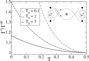
Figure 2: The ratio of the local to the non-local decoherence rate is shown as a function of the transmission ${\cal T}$ at the beam splitters for different values of the incoherent parallel resistance $1/T_{0}$. All curves are symmetric with respect to ${\cal T}=1/2$. In the inset, the two possible electron paths at the beam splitter and the resistance $1/T_{0}$ (in units of $h/e^{2}$) are indicated. After Ref. [13], copyright (2003) by the American Physical Society.

With these assumptions we obtained for the dephasing rates in the local ($\it l$) and non-local ($\it nl$) configuration respectively,

$$\Gamma^{l}_{\phi}=\gamma^{0}_{\phi}+\gamma^{l}_{\phi}, \,\,\,\gamma^{l}_{\phi}=\gamma^{0}_{\phi}\,\frac{(2{\cal T}-1)^{2}}{2{\cal T}(1-{\cal T})+T_{0}},$$ (19a)

$$\Gamma^{nl}_{\phi}=\gamma^{0}_{\phi}+\gamma^{nl}_{\phi}, \,\,\,\gamma^{nl}_{\phi}=\gamma^{0}_{\phi}\,\frac{(2{\cal T}-1)^{2}}{1+2T_{0}}.$$ (19b)

Here, $\gamma^{l}_{\phi}$ and $\gamma^{nl}_{\phi}$ are the probe-configuration specific contributions. The experiment of Ref. [4] shows transmission between neighbouring contacts to be significant. For better comparison, we therefore included a finite incoherent transmission $T_{0}=T_{12}=T_{21}=T_{34}=T_{43}$ (see inset Fig. 2). In our calculations we have assumed that both beam splitters are identical but relaxing this condition will not change the results qualitatively.

The decoherence rate in the local (19a) and non-local configuration (19b) is higher than in the voltage biased configuration (18). This can be understood as an enhancement of the charge relaxation resistance $R_{q}$. Attaching a high-ohmic voltmeter and thus closing some exits of the MZI will render charge relaxation more difficult.

The decoherence rates Eq. (19) are strongly dependent on the symmetry of the beam splitters. For perfectly symmetric beam splitters ${\cal T}=1/2$ the two configurations are equivalent and the dephasing rate in both cases is simply given by $\gamma^{0}_{\phi}$. In the opposite limit of strong asymmetry (${\cal T}\rightarrow 0$ or ${\cal T}\rightarrow 1$) however, the local decoherence rate is greatly enhanced over the non-local decoherence rate due to the symmetry-dependent denominator in the configuration specific part of the dephasing rate. The divergence of the local decoherence rate for ${\cal T}=0$ and ${\cal T}=1$ is cut off by an incoherent parallel transmission $T_{0}$. The ratio of the local to the non-local decoherence rate is shown in Fig. 2 for different values of $T_{0}$. It should be emphasized that the difference between the local and non-local configuration survives even if the intersections are not treated as ideal beam splitters but exhibit a certain degree of randomness [13].

3 An interferometer with chaotic scattering

So far we have investigated the electronic equivalent of the optical MZI and we have shown how charge fluctuations lead to decoherence. In this section we want to consider a different type of interferometer shown in Fig. 3. As in the case of the MZI the region where the external leads are connected to the ring is modelled by a beam splitter (see Eq. (1)). An electron coming from an external lead will thus enter the ring with certainty and an electron arriving at the intersection from the ring will go out into one of the reservoirs. This implies that any given electron can go around the ring exactly once. An electron going through the ring clockwise picks up a phase $k_{F}L+2\pi\Phi$ and an electron going through the ring counter-clockwise picks up a phase $k_{F}L-2\pi\Phi$ (for simplicity we have assumed this phase to be the same for all channels). Interference will be due to electron-trajectories enclosing the ring clockwise with trajectories going around the ring in the counter-clockwise direction. To mimic the backscattering and channel mixing that is always present in an experiment (see e.g. Ref. [3, 4]) a chaotic dot is embedded into the arm of the ring. We will in the following assume that all interactions take place in the quantum dot and no interactions take place in the ring. Restricting the interactions to the quantum dot can certainly be justified if the dwell time in the dot is long compared to the traversal time for the ring. If we furthermore assume that the hole in the ring is large compared to the surface of the chaotic dot, a magnetic flux of the order of one flux quantum through the ring will not break time-reversal invariance in the dot. The (time-independent) scattering matrices for the dot are then distributed according to the circular orthogonal ensemble.

Figure 3: Mesoscopic interferometer with a chaotic dot integrated in its arm. The dot is capacitively coupled to a gate and interactions are taken into account through a self-consistent internal potential $U(t)$. The paths an electron incoming from the left lead can take are also indicated.

As in Sec. 2.3 we will treat interaction effects on the level of the single potential approximation. We thus characterize the quantum dot by an internal potential $U(t)$ that has to be determined self-consistently. For an open chaotic dot in the many channel limit this approximation is well justified [19, 20]; it is in fact very common in the study of Coulomb blockade problems. In the many-channel limit the potential can be considered as a Gaussian random variable with a spectrum $\Sigma_{UU}(\omega)$ [21]. In the presence of a time-dependent internal potential we have to use scattering matrices $S(t,t^{\prime})$ with two time arguments to describe scattering in the dot. Since we assume that no scattering takes place in the ring, the scattering matrix for the ring is a diagonal matrix with elements $S_{nn}(t,t^{\prime})=\delta(t-t^{\prime}-L/v_{F}){\rm e}^{ik_{F}L\pm 2i\pi\Phi}$ (see Eq. (9), the positive (negative) sign is for an electron going around the ring in the (counter-) clockwise direction and $n$ is the channel index). The ensemble averaged conductance can then be calculated using the time-dependent scattering matrix theory of Ref. [16]. In this calculation we will need correlators of the type $\langle S_{ij}(t,t^{\prime})S^{\ast}_{kl}(s,s^{\prime})\rangle$ which can be found there. After performing both an ensemble average and – in addition – a statistical average over the (Gaussian) potential fluctuations we obtain for the conductance

$$\frac{G}{G_{0}}=-\frac{N}{2}+\frac{(1-2{\cal T})^{2}}{4}+A_{\phi}{\cal T}(1-{\cal T})\cos(4\pi\Phi).$$ (20)

Here, we have assumed that an equal number of channels $N\gg 1$ is open in all the leads. From Eq. (20) we see that on the ensemble average there is no coherent (flux-dependent) contribution to the leading order term of the conductance. Furthermore, the fluctuating internal potential only affects the flux-dependent part of the weak localization correction to the conductance. The amplitude

$$A_{\phi}=\left\{\begin{array}[]{ll}\left(1+2\tau_{d}\Gamma_{\phi}\right)^{-1},&\tau\gg\tau_{d},\\ \exp\left(-2\tau\Gamma_{\phi}\right),&\tau\ll\tau_{d}.\end{array}\right.$$ (21)

depends on the strength of the decoherence and can in principle be obtained exactly. Here, we concentrated on the two interesting limits $\tau\gg\tau_{d}$ and $\tau\ll\tau_{d}$. where $\tau_{d}=h/(2N\Delta)$ is the dwell time, $\Delta$ is the level spacing in the dot and $\tau=L/v_{F}$ is the traversal time for the ring. The decoherence rate $\Gamma_{\phi}=e^{2}\Sigma_{UU}(0)/2\hbar^{2}$ is defined as in Eq. (17).

A single (time-dependent) potential $U(t)$ can not introduce a phase difference between interfering trajectories confined to a quantum dot and will therefore not suppress or dephase the weak localization correction to the conductance. To understand the experimental results for dephasing in chaotic dots of Refs. [22, 23, 24] one thus has to go beyond the single potential approximation. In our more complicated model, however, it is possible that electrons on different trajectories through the ring pass through the dot at different times. In this situation, dephasing due to a single fluctuating potential in the dot becomes effective. The time during which two interfering electrons are exposed to different potentials $U(t)$ is given by the minimum of the dwell time $\tau_{d}$ and the traversal time $\tau$. In the limit $\tau\gg\tau_{d}$ the amplitude $A_{\phi}$ becomes independent of the traversal time $\tau$ and therefore of the circumference $L$ of the ring. This is a consequence of our assumption that interactions are restricted to the dot. In the opposite limit, $\tau\ll\tau_{d}$, the amplitude $A_{\phi}$ depends exponentially on the traversal time but is independent of the dwell time.

For zero magnetic field and if $\tau\rightarrow 0$ and thus $A_{\phi}\rightarrow 1$ the system reduces to a simple chaotic dot and the fluctuating potential has no effect whatsoever. In this case, the weak localization correction is $1/4$ as was first obtained from a scattering matrix approach in Refs. [25, 26]. In the limits ${\cal T}\rightarrow 0$ or ${\cal T}\rightarrow 1$ the system corresponds to a simple quantum dot with two external leads even for arbitrary traversal time and magnetic field. For strong dephasing, $A_{\phi}=0$, the weak localization correction of Eq. (20) is $(1-2{\cal T})^{2}/4$. It can be obtained from the incoherent addition of the four different paths between the two external contacts. (Note, that even in this ”incoherent” regime coherent backscattering does take place in the dot).

In an experiment it might be interesting to vary the location of the quantum dot. Decoherence due to a single fluctuating potential should be strongly suppressed in a perfectly symmetric interferometer where the dot is connected to the beamsplitter by two arms of exactly the same length. In such a setup time-reversal symmetry would not be broken and even the flux-dependent term would not be dephased.

The low-frequency dynamics of the charge fluctuations in the dot is governed by a charge relaxation time $\tau_{RC}=R_{q}C_{\mu}$. In a multi-channel chaotic dot the charge relaxation time is much shorter than the dwell time $\tau_{d}$ ($\tau_{RC}\ll\tau_{d}$). For the interferometer considered here, we have in addition $\tau_{RC}\ll\tau$. It is this separation of time scales that allows us to relate the decoherence rate to the zero-frequency limit of the spectral function only. The potential fluctuation spectrum $\Sigma_{UU}(\omega)$ for a chaotic dot can be found with the help of Ref. [27] where the dynamic conductance matrix for a chaotic dot capacitively coupled to a gate was calculated. The fluctuation dissipation theorem in the classical limit gives $\Sigma_{UU}(\omega)=2kT{\rm Re}G_{GG}(\omega)/(C^{2}\omega^{2})$ where $G_{GG}(\omega)$ is the matrix element relating the current induced into the gate to a variation of the gate voltage. In the zero-frequency limit the spectral function for the charge fluctuations in the dot is $\Sigma_{UU}(0)=2kTR_{q}(C_{\mu}/C)^{2}$. The charge relaxation resistance for a dot attached to two leads with $N$ channels each is $R_{q}=(h/e^{2})/(2N)$. It is thus just the parallel addition of the resistances $(h/e^{2})/N$ of the individual contacts. Furthermore, the electrochemical capacitance $C_{\mu}$ is the series addition of the geometrical capacitance $C$ and the density of states $e^{2}D$ ($D=\Delta^{-1}$), namely $C^{-1}_{\mu}=C^{-1}+(e^{2}D)^{-1}$ [18]. In the experimentally relevant limit $C_{\mu}/C\rightarrow 1$ we thus get

$$\Gamma_{\phi}=\frac{\pi kT}{\hbar N}.$$ (22)

The dependence of the dephasing rate on the size of the contacts, i.e. on $N$, reflects the fact that potential fluctuations in the dot are the smaller the larger the contacts.

It is interesting to compare Eq. (20) with the result obtained if dephasing is introduced via a voltage probe model [28, 29, 30]. In this model a fictitious voltage probe is connected to the dot. It is imposed that no net current flows at this terminal such that every outgoing electron has to be replaced by an incoming one. The two exchanged electrons have however no phase-relation which leads to a suppression of coherence in the dot. Using the diagrammatic theory of Ref. [31] it is possible to calculate the average conductance of the system including the voltage probe and we obtain

$$\frac{G}{G_{0}}=-\frac{N}{2}+\frac{2N}{2N+\gamma}\left[\frac{(1-2{\cal T})^{2}}{4}+{\cal T}(1-{\cal T})\cos(4\pi\Phi)\right].$$ (23)

Note that in the limits ${\cal T}\rightarrow 0$ and ${\cal T}\rightarrow 1$ we correctly recover the result for the conductance of a simple chaotic dot. In contrast to a single fluctuating potential the voltage probe leads to decoherence of the full weak-localization correction. In principle one could also attach the voltage probe directly to the ring instead of attaching it to the quantum dot. In this case the result would be similar to Eq. (20) since a voltage probe attached to the ring will not suppress interference between trajectories in the dot.

4 Conclusions

In this work we have investigated charge-fluctuation-induced decoherence of AB oscillations in mesoscopic interferometers. As a first example we looked at an interferometer without backscattering, the electronic equivalent of an optical Mach-Zehnder interferometer. Employing a time-dependent scattering approach we have been able to relate the suppression of coherent Aharonov-Bohm oscillations to the spectrum of internal potential fluctuations. Then, specializing to the case where both arms of the ring are described by a single potential each, we have explicitly calculated the decoherence rate. Within our model the decoherence rate is linear in temperature as observed in Refs. [3, 4]. We also demonstrated that the potential fluctuations and thus the decoherence rate can strongly depend on the external measurement circuit. This provides an explanation of the measurement configuration dependence of the decoherence rate in a four-terminal mesoscopic ring reported in Ref. [4].

As a second example we studied a mesoscopic ring with a chaotic dot included in its arm. This has allowed us to take into account backscattering and channel mixing. Also, contrary to the case of the MZI where we were mainly interested in the single-channel limit, we have allowed for a large number of channels in the ring. Making the assumption that interactions take place mainly in the dot and describing the dot by a single internal potential we could again relate the decoherence rate to the potential fluctuation spectrum.

It is important to emphasize that the conductors considered here do not have to be charge neutral. To the contrary, an open mesoscopic conductor can easily be charged up relative to its surroundings by exchanging charge with the reservoirs. Charge exchange between conductor and reservoir is an important source of dephasing. This is reflected in the dependence of the dephasing rates we have calculated above on the charge relaxation resistance $R_{q}$. The charge relaxation resistance is a measure of the energy dissipated as a charge carrier relaxes into a reservoir. Charge relaxation becomes easier the more channels are open in the leads connecting conductor and reservoirs. In consequence deviations from charge neutrality are evened out quicker and charge fluctuations become less pronounced. This, in turn leads to a smaller decoherence rate.

There are many interesting venues leading beyond the material presented here. Clearly, it would be interesting to go beyond the single potential approximation to determine the decoherence rate for a mesoscopic interferometer. Such a generalization would become necessary if one was interested to know how charge fluctuations suppress the weak localization correction to the conductance of a quantum dot.

References

- [2]
- [3] A. E. Hansen, A. Kristensen, S. Pedersen, C. B. Sorensen, and P. E. Lindelof, Phys. Rev. B 64 (2001) 045327.
- [4] K. Kobayashi, H. Aikawa, S. Katsumoto, and Y.Iye, J. Phys. Soc. Jpn. 71 (9) (2002) 2094.
- [5] Y. Ji, Y. Chung, D. Sprinzak, M. Heiblum, D. Mahalu and H. Shtrikman, Nature 422 (2003) 415.
- [6] F. Marquardt and C. Bruder, cond-mat/0306504.
- [7] P. Samuelsson, E. Sukhorukov, and M. Büttiker, Phys. Rev. Lett. 91, (2003) 157002.
- [8] J. L. van Velsen, M. Kindermann, and C. W. J. Beenakker, cond-mat/0307103.
- [9] V. Scarani, N. Gisin, and S. Popescu, cond-mat/0307385.
- [10] P. Samuelsson, E. Sukhorukov, and M. Büttiker, cond-mat/0307473.
- [11] J. J. Lin and J. P. Bird, J. Phys. Condens. Matter 14 (2002) R501.
- [12] G. Seelig and M. Büttiker, Phys. Rev. B 64, (2001) 245313.
- [13] G. Seelig, S. Pilgram, A. N. Jordan and M.Büttiker, Phys. Rev. B 68, (2003) 161310(R).
- [14] B. L. Altshuler, A. G. Aronov and, D. Khmelnitskii, J. Phys. C 15 (1982) 7367.
- [15] M. Büttiker, H. Thomas, and A. Prêtre, Z. Phys. B 94 (1994) 133.
- [16] M. L. Polianski and P. W. Brouwer, J. Phys. A: Math. Gen. 36 (2003) 3215.
- [17] M. G. Vavilov and I. L. Aleiner, Phys. Rev. B 60 (1999) R16 311.
- [18] M. Büttiker, H. Thomas, and A. Prêtre, Phys. Lett. A 180 (1993) 364.
- [19] Y. M. Blanter, Phys. Rev. B 54 (1996) 12807.
- [20] I. L. Aleiner, P. W. Brouwer and L. I. Glazman, Phys. Rep. 358 (2002) 309.
- [21] Non-Gaussian charge fluctuations in many channel chaotic cavities have recently been investigated by S. Pilgram and M. Büttiker, Phys. Rev. B 67 (2003) 235308.
- [22] J. P. Bird, K. Ishibashi, D. K. Ferry, Y. Ochiai, Y. Aoyagi, and T. Sugano, Phys. Rev. B 51 (1995) 18 037.
- [23] R. M. Clarke, I. H. Chan, C. M. Marcus, C. I. Duruöz and J. S. Harris, Jr., K. Campman, and A. C. Gossard, Phys. Rev. B 52 (1995) 2656.
- [24] A. G. Huibers, M. Switkes, C. M. Marcus, K. Campman, and A. C. Gossard, Phys. Rev. Lett. 81 (1998) 200.
- [25] H. U. Baranger and P. A. Mello, Phys. Rev. Lett. 73 (1994) 142.
- [26] R. A. Jalabert, J.-L. Pichard, C. W. J. Beenakker, Europhys. Lett. 27 (1994) 255.
- [27] P. W. Brouwer and M. Büttiker, Europhys. Lett. 37 (1997) 441.
- [28] M. Büttiker, Phys. Rev. B 33 (1986) 3020; IBM J. Res. Dev. 32 (1988) 63.
- [29] H. U. Baranger and P. A. Mello, Phys. Rev. B 51 (1995) 4703.
- [30] P. W. Brouwer and C. W. J. Beenakker, Phys. Rev. B 51 (1995) 7739.
- [31] P. W. Brouwer and C. W. J. Beenakker, J. Math. Phys. 37 (1996) 4904.