Empirical basis for car-following theory development

Abstract

By analyzing data from a car-following experiment, it is shown that drivers control their car by a simple scheme. The acceleration $a(t)$ is held approximately constant for a certain time interval, followed by a jump to a new acceleration. These jumps seem to include a deterministic and a random component; the time $T$ between subsequent jumps is random, too. This leads to a dynamic, that never reaches a fixed-point ($a(t)\to 0$ and velocity difference to the car in front $\Delta v\to 0$) of the car-following dynamics. The existence of such a fixed-point is predicted by most of the existing car-following theories. Nevertheless, the phase-space distribution is clustered strongly at $\Delta v=0$. Here, the probability distribution in $\Delta v$ is (for small and medium distances $\Delta x$ between the cars) described by $p(\Delta v)\propto\exp(-|\Delta v|/\Delta v_{0})$ indicating a dynamic that attracts cars to the region with small speed differences. The corresponding distances $\Delta x$ between the cars vary strongly. This variation might be a possible reason for the much-discussed widely scattered states found in highway traffic.

I Introduction

To understand traffic flow, it is mandatory to analyze the interaction between the cars. The simplest of these interactions is car-following, where a car with speed $v$ follows a lead car with speed $V$ in a certain distance $\Delta x$. Although a lot of theoretical work has been undertaken to describe this process (see Chowdhury ; Helbing ; OR-review for reviews), these models have a weak empirical basis. Often, calibration and validation is done only qualitatively, or by comparing the model’s output with macroscopic data like counts and average speeds from induction loop detectors.

The models introduced so far may be classified according to the update scheme of the underlying dynamic as cellular automata, differential equations and their time-discretization, and as so called action-point models Todosiev1963 ; Michaels1963 . All models describe the car-following process by an equation for the acceleration $a$ of the following car, $a=a\left(\Delta x,v,V\right)$. In case of a stochastic model, the (white) noise is added to the acceleration, making $a(t)$ discontinuous in time. Only the action-point models differ from that, they claim the acceleration more or less constant until a certain action-point is reached where the acceleration changes within a short amount of time.

In the following, a new data-set will be analyzed that allows a detailed analysis of the car-following process. This gives important hints how the car-following description can be improved at least on the microscopic level.

II Results of data analysis

The data to be analyzed have been described in DGPS-RTK : a platoon of ten cars, each equipped with differential GPS, drove along a test track and recorded some hours of car-following data. The time resolution of the data is 0.1 s, while the accuracy in position of 0.1 m. For each car $n$, its position $x_{n}(t)$ and speed $v_{n}(t)$ along the test track is recorded. The driver of the lead car was instructed to drive certain speed patterns to estimate the reaction of the following cars. All drivers were fully informed about the experiment.

Note, that the data contain only the gross headway $\Delta x_{n}=x_{n-1}-x_{n}$, i.e. the distance from GPS-receiver to GPS-receiver, but not the car lengths. From the speed data, the acceleration has been computed by applying a symmetric Savitzky-Golay filter Press_NR .

II.1 Distribution of speed differences

The trajectories of the cars in the phase-space $(\Delta v,\Delta x)$ display an oscillatory behavior, see Todosiev1963 ; Brackstone2002 (and references therein) for similar observations.

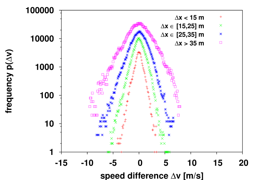
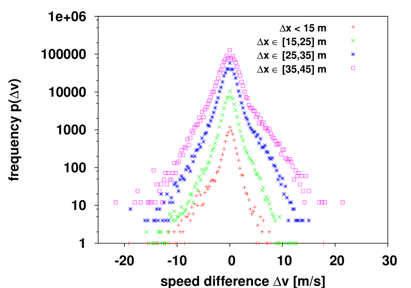
Figure 1: The histogram $p_{\Delta x}(\Delta v)$ of the velocity difference for different distances $\Delta x$ between the cars. The upper plot is for the GPS data, the lower plot shows the result for single car data from the German freeway A1 Schadschneider-data . The different curves have been scaled to increase visibility.

However, these oscillations cannot be understood as a noisy limit-cycle, as can be seen by analyzing the frequency distribution of the velocity difference $p_{\Delta x}(\Delta v)$. This distribution is non-analytic for small distances $\Delta x<30$ m (for the test track data, for data from the highway this behavior can be observed for even bigger distances), while there is a cross-over to a more Gaussian behavior for larger distances, see Fig. 1. Most car-following models claim that there is a fixed-point $g^{\star}$ of the car-following dynamics where $a=0,\Delta v=0$ and the distance to the car ahead is given by some function $g^{\star}(v)$. This idea can be tested easily with the data at hand, and it is wrong. Although the cars “like” $\Delta v=0$, they don’t get stuck there. The data-points where $\Delta v$ and $a$ are small (the classical hallmark of a fixed point) are just part of a very short sequence of one or two data-points of the time-series of $\Delta v(t)$ and $a(t)$, respectively. The reason for this can be inferred from the time-series of the acceleration $a(t)$, see Fig. 2.

Figure 2: The acceleration $a(t)$ drawn as a function of time. The action-points have been determined from $a(t)$ by searching local minima/maxima of $\dot{a}$ where $|\dot{a}|>\sigma$, where $\sigma$ is the noise in $\dot{a}$. Additionally, to any sequence of points where $|\dot{a}|>\sigma$ only one minimum/maximum has been assigned to suppress spurious minima/maxima.

This time-series can be understood as a sequence of pieces where acceleration is essentially constant (or a linear function of time) and fast transitions between these pieces. Since this phenomenon has been described already in Todosiev1963 ; Michaels1963 , who named these points “action-points”, this name will be used in the following.

The pieces where acceleration is not constant, but a linear function of time can be understood as episodes where the driver does not change the amount of gas or brake. Because of friction, the acceleration (positive acceleration increases speed and this increases friction, lowering acceleration) will change then over time. However, not all possible values of acceleration are equally likely, e.g. a small negative value (increasing as a function of speed $a_{0}\propto-c_{1}v$) is chosen much more often. It can be speculated, that these values belong to a state where the driver is doing nothing, neither touching gas nor brake.

II.2 Waiting times

The times $T_{i}$ between subsequent decisions to change acceleration have been obtained by the algorithm described in Fig. 2. In Fig. 3, the corresponding frequency distribution is displayed. The exponential tail of this distribution indicates that any decision is independent from the proceeding one, with one exception: the probability for making a new decision right after an action-point is reduced.

More detailed inspections show that the mean-value averaged over all the drivers is $\langle T\rangle=2.5\,s$, with large differences between drivers ranging from $T=1.8\ldots 4\,s$. Interestingly, the waiting time between action-points seems to be independent of distance or speed difference.

Figure 3: The waiting time distribution between subsequent action-points.

II.3 Acceleration

The acceleration data are consistent with a simple linear relationship

$$a(\Delta x,\Delta v)\propto a_{g}(g^{\star}(v)-\Delta x)+a_{\Delta v}\Delta v.$$ (1)

However, this is only the average behavior, the corresponding standard deviation $\sigma_{a}$ of the estimated acceleration values is usually fairly big. This indicates once more that the whole car-following process can be described as a stochastic process.

The analysis of the jumps in $a(t)$ lends further support to this claim. The jumps are scattered (see Fig. 5) in the whole $(\Delta v,\Delta x)$-space. Fig. 4 displays the distribution of the jump-sizes. Also in this figure is a comparison to a Gaussian distribution which indicates that the jump-size distribution is not Gaussian.

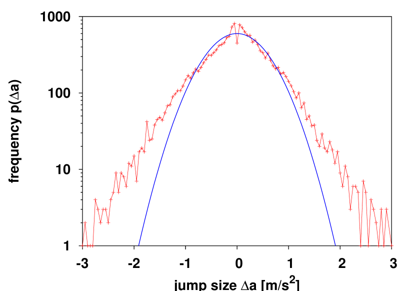
Figure 4: The frequency distribution $p(\Delta a)$ of the acceleration jumps $\Delta a$. Also shown is a fit of these data to a Gaussian distribution.

III Reflections on modeling

The results above are inconsistent with most existing microscopic car-following models. The models claim that the car-following process tends to converge to some preferred distance $g^{\star}(v)$ which depends on speed. In some models, and for some ranges of speed, this fixed-point is unstable, giving rise to an instability which may finally be responsible for jam formation. Other models have more than one fixed point, which has been hypothesized K2 ; K2W as the reason for the widely scattered states commonly known as synchronized flow. Since the data above show that there is no such fixed point, on a microscopic level all these models are inconsistent with the data. Of course, under a certain amount of course graining a region $[g^{\star}_{\text{min}},g^{\star}_{\text{max}}]$ may serve as a substitute for a fixed point. However, definitive conclusions concerning the macroscopic consequences of the microscopic behavior found here can be drawn only after suitable models have been constructed that embed the behavior above in their dynamics.

As mentioned already, the so-called action-point models Todosiev1963 ; Michaels1963 behave indeed differently. They are built around the idea of a constant acceleration between the action-points, which seems to be in line with the observations above. Usually, the action-point models include the idea of so-called perception thresholds in human perception. The most important threshold $\theta_{\Delta v}$ is the one for determining small changes in speed difference. It is defined by the equation $\theta_{\Delta v}\propto\Delta v/(\Delta x)^{2}$. Although this sounds like a firm psycho-physical basis, the data above and the data of others Brackstone2002 do not support the idea of those thresholds. Note, however, that the analysis in Brackstone2002 claims to have found empirical evidence for those thresholds, however from inspecting their results different conclusions may be drawn as well. In Fig. 5, all the action-points have been drawn in $(\Delta v,\Delta x)$-space. Their distribution coincides with the one of all the data-points. Even more, the action-points for increasing acceleration and the ones for decreasing acceleration cover almost the same area. Only when action-points with large absolute values of acceleration are plotted, then some clustering of the points can be seen.

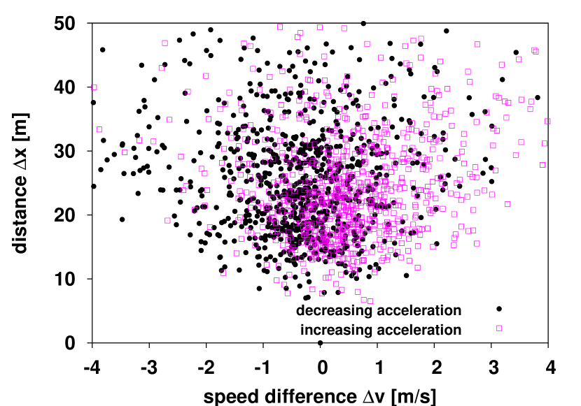
Figure 5: The action-points in the $(\Delta v,\Delta x)$-plane.

A more likely interpretation is the idea that the thresholds are in the space of driving strategies, of which the chosen acceleration may be a proxy. If the chosen strategy becomes too uncomfortable, then a new one is chosen. First ideas in this direction have been put forward already BRDM ; RDM .

From the findings above, more realistic car-following models can be constructed. They consist of an acceleration law that determines the optimal or desired acceleration as function of speed, speed difference, and distance. Based on the analyses performed so far, no definitive acceleration model could be favored or ruled out.

So, any of the previously invented car-following models could be used here, too. What has to be added, is a specific noise-term that acts not on acceleration directly, but works on the basis of events: after a certain randomly chosen time $T$, a new desired acceleration is set. This desired acceleration has a strong stochastic part, from the data no unique average (optimal) acceleration could be determined so far.

After setting the acceleration to its new value, it remains constant until the next decision has to be made. The relaxation between two subsequent values is compatible with a simple relaxation $\dot{a}=(a_{\text{des}}-a)/\tau_{a}$, since the time $\tau_{a}$ is of the order of 0.5 s, even the usage of time-discrete models can justified. Results based on these ideas will be presented in future work.

IV Conclusions

This work has analyzed experimental car-following data that were obtained under idealized conditions. Wherever possible, the results found have been tried to back up by using similar data that have been obtained from other sources such as highway data. Additional data have been considered as well, but were not reported here, since they confirm the analysis done here. Anything taken together, the results obtained are sufficiently general to support the following conclusions. The process of car-following can be described by a relatively simple dynamical process that controls the acceleration. From time to time, the driver computes a new desired acceleration (which of course refers to a specific configuration of the gas and brake pedal) which consists of a deterministic and a random part. The times between subsequent decisions are randomly distributed, too. The deterministic part is responsible for the presence of the car near $\Delta v=0$ which is a very prominent feature in the data. The random part competes with this approach to $\Delta v=0$. It works that strong, that in fact no fixed point of the car following dynamics can be established, because acceleration only by chance becomes zero, and this does not last for a long time.

The consequences for microscopic modeling have been derived, indications how to construct models that comply with these data have been given. A much more difficult task for future research is to find out how exactly the choice of strategies is being performed, and how big the stochastic component of this choice is.

Finally, the findings presented here may shed a new light on the discussion about widely scattered states in traffic flow. Simulations based on a simple model consistent with the findings above display widely scattered states. We hope to report on this work in future contributions. However, the question about stability of traffic flow has to be answered, and it cannot be discussed simply by a linear stability analysis. The action-point dynamic of human driving on one hand has a tendency to produce fluctuations that might destroy homogeneous traffic flow. On the other hand, since the car-following dynamic converges to a small region in phase-space, at least small perturbations can heal out. So, the idea that traffic flow is just at the border of instability got a new meaning.

References

- (1) D. Chowdhury, L. Santen, and A. Schadschneider, Phys. Rep. 329, 199 (2000).
- (2) D. Helbing, Rev. Mod. Phys. 73, 1067 (2001).
- (3) K. Nagel, P. Wagner, and R. Woesler, Oper. Res. 51 (2003).
- (4) E. P. Todosiev, and L. C. Barbosa, Traffic Engineering 34, 17 – 20 (1963/64).
- (5) R. M. Michaels, Proceedings of the second international symposium on the theory of road traffic flow, 44-59, OECD (1963).
- (6) G. S. Gurusinghe, T. Nakatsuji, Y. Azuta, P. Ranjitkar, and Y. Tanaboriboon, Transp. Res. Board conference 2003, paper # TRB2003-004137 (2003).
- (7) W. H. Press, S. A. Teukolsky, W. T. Vetterling, and B. P. Flannery, “Numerical Recipes in C”, Cambridge University Press, 2nd edition (1992).
- (8) M. Brackstone et al., Transp. Res. F 5 329-344 (2002).
- (9) W. Knospe, L. Santen, A. Schadschneider, and M. Schreckenberg, Phys. Rev. E 65 056133 (2002).
- (10) B. S. Kerner and S. L. Klenov, J. Phys. A 35, L31 - L43 (2002).
- (11) B. S. Kerner, S. L. Klenov, and D. W. Wolf, J. Phys. A: Math. Gen, 35, 9971-10013 (2002)
- (12) I. Lubashevsky, P. Wagner, and R. Mahnke, Europ. Phys. J. B 32 243 – 247 (2003).
- (13) I. Lubashevsky, P. Wagner, and R. Mahnke, Phys. Rev. E 68 ?? (2003).
- (14) H. T. Fritzsche, Traf. Eng. Contr. 5, 317 (1994).
- (15) W. Leutzbach and R. Wiedemann, Traf. Eng. Contr., 27, 270-278 (1986).