A stochastic cellular automaton model for traffic flow with multiple metastable states

Abstract

A new stochastic cellular automaton (CA) model of traffic flow, which includes slow-to-start effects and a driver’s perspective, is proposed by extending the Burgers CA and the Nagel-Schreckenberg CA model. The flow-density relation of this model shows multiple metastable branches near the transition density from free to congested traffic, which form a wide scattering area in the fundamental diagram. The stability of these branches and their velocity distributions are explicitly studied by numerical simulations.

1 Introduction

Traffic problems have been attracting not only engineers but also physicists [1]. Especially it has been widely accepted that the phase transition from free to congested traffic flow can be understood using methods from statistical physics [2, 3]. In order to study the transition in detail, we need a realistic model of traffic flow which should be minimal to clarify the underlying mechanisms. In recent years cellular automata (CA) [4, 5] have been used extensively to study traffic flow in this context. Due to their simplicity, CA models have also been applied by engineers, e.g. for the simulation of complex traffic systems with junctions and traffic signals [6].

Many traffic CA models have been proposed so far [2, 7, 8], and among these CA, the deterministic rule-184 CA model (R184), which is one of the elementary CA classified by Wolfram [4], is the prototype of all traffic CA models. R184 is known to represent the minimum movement of vehicles in one lane and shows a simple phase transition from free to congested state of traffic flow. In a previous paper [9], using the ultra-discrete method [10], the Burgers CA (BCA) has been derived from the Burgers equation

$$v_{t}=2vv_{x}+v_{xx},$$ (1)

which was interpreted as a macroscopic traffic model [11]. The BCA is written using the minimum function $\min$ by

$$U_{j}^{t+1}=U_{j}^{t} + \min\{U_{j-1}^{t},L-U_{j}^{t}\}-\min\{U_{j}^{t},L-U_{j+1}^{t}\},$$ (2)

where $U_{j}^{t}$ denotes the number of vehicles at the site $j$ and time $t$. If we put the restriction $L=1$, it can be easily shown that the BCA is equivalent to R184. Thus we have clarified the connection between the Burgers equation and R184, which offers better understanding of the relation between macroscopic and microscopic models.

The BCA given above is considered as the Euler representation of traffic flow. As in hydrodynamics there is an another representation, called Lagrange representation [12], which is specifically used for car-following models. The Lagrange version of the BCA is given by [13]

$$x_{i}^{t+1}=x_{i}^{t}+\min\{V_{max},x^{t}_{i+S}-x^{t}_{i}-S\},$$ (3)

where $V_{max}=S=L$ and $x^{t}_{i}$ is the position of $i$-th car at time $t$. Note that in (3) $S$ corresponds a “perspective” or anticipation parameter [14] which represents the number of cars that a driver sees in front, and $V_{max}$ is the maximum velocity of cars. (3) is derived from the BCA mathematically by using an Euler-Lagrange (EL) transformation [13] which is a discrete version of the well-known EL transformation in hydrodynamics.

In this paper, we will develop the BCA (3) to a more realistic model by introducing slow-to-start (s2s) effects [15, 16, 17, 18] and a driver’s perspective $S$. Moreover, a stochastic generalization is also considered by combining it with the Nagel-Schreckenberg (NS) model [8, 19].

2 Traffic models in Lagrange form

First, let us extend (3) to the case $V_{max}\neq S$ and combine it with the s2s model. The s2s model [12] is written in Lagrange form as

$$x_{i}^{t+1} = x_{i}^{t}+\min\{1,x^{t}_{i+1}-x^{t}_{i}-1,x^{t-1}_{i+1}-x^{t-1}_{i}-1\}.$$ (4)

Note that the inertia effect of cars is taken into account in this model. Comparing (4) and (3), we see that, in the s2s model, the velocity of a car depends not only on the present headway $d_{i}^{t}=x^{t}_{i+1}-x^{t}_{i}-1$, but also on the past headway $d_{i}^{t-1}=x^{t-1}_{i+1}-x^{t-1}_{i}-1$. This rule has only a nontrivial effect if $d_{i}^{t-1}=0$ and $d_{i}^{t}=1$, i.e. if the leading car has started to move in the previous time step. In this case the following car is not allowed to move immediately (s2s).

Before combining (3) and (4), it is worth pointing out that we can choose the perspective parameter as $S=2$ in the model according to observed data. We define the size of a cell as 7.5 m and $V_{max}=5$ in our model according to the NS model. Since $V_{max}$ corresponds to about 100 km/hour in reality, then one time step in the CA model becomes 1.3 s. Moreover, the gradient of the free line and jamming line in the fundamental diagram, which is the dependence of the traffic flow $Q$ on density $\rho$, is known to be about 100 km/hour and $-15$ km/hour [3] according to many observed data (see Fig. 1) [20, 21]. These values correspond to the typical free velocity and the jam velocity, respectively.

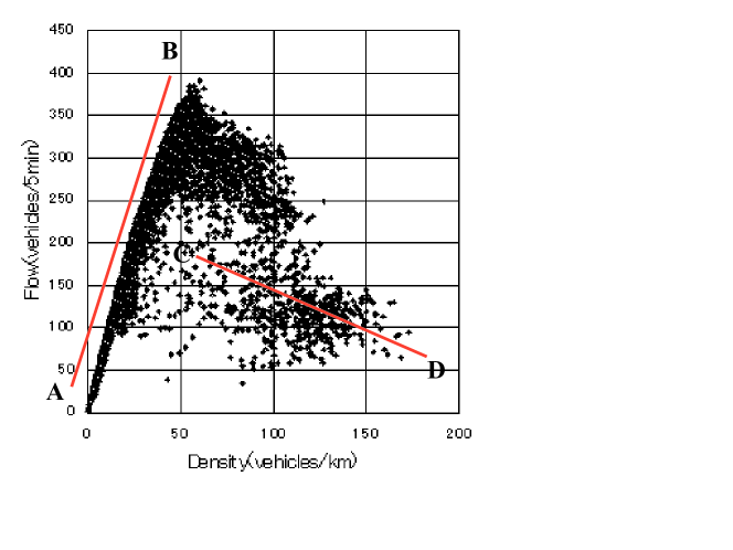
Figure 1: An observed fundamental diagram at the Tomei expressway in Japan. The gradient of the free line ($A-B$) and jamming line ($C-D$) is known to be about 100 km/hour and $-15$ km/hour. We also see that there is a wide scattering area near the phase transition region from free to jamming state.

Thus, considering the fact that the positive and negative gradient of each line is given by $V_{max}=5$ and $-S/2$, respectively, in the CA model [12], we should choose $S=1.5$ in the CA model. Since only integer numbers for $S$ are allowed in this model, we will simply choose $S=2$ for studying the effect of the perspective of drivers. It is noted that other possibilities, such as velocity-dependent $S$ or stochastic choice of $S$, are also possible.

Now by combining (3) and (4) we propose a new Lagrange model with $S=2$ which is defined by the rules listed below: Let $v^{(0)}_{i}$ be the velocity of the $i$-th car at a time $t$. The update procedure from $t$ to $t+1$ is divided into five stages:

1. Accerelation

   $$v^{(1)}_{i}=\min\{V_{max},v^{(0)}_{i}+1\}.$$ (5)

2. Slow-to-accelerate effect

   $$v^{(2)}_{i}=\min\{v^{(1)}_{i},x^{t-1}_{i+2}-x^{t-1}_{i}-2\}.$$ (6)

3. Deceleration due to other vehicles

   $$v^{(3)}_{i}=\min\{v^{(2)}_{i},x^{t}_{i+2}-x^{t}_{i}-2\}.$$ (7)

4. Avoidance of collision

   $$v^{(4)}_{i} = \min\{v^{(3)}_{i},x^{t}_{i+1}-x^{t}_{i}-1+v^{(3)}_{i+1}\}$$ (8)

5. Vehicle movement

   $$x_{i}^{t+1}=x_{i}^{t}+v^{(4)}_{i}.$$ (9)

The velocity $v^{(4)}_{i}$ is used as $v^{(0)}_{i}$ in the next time step. (8) is the condition that the $i$-th car does not overtake its preceding $(i+1)$-th car, including anticipation. The accerelation (5) is the same as in the NS model, which is needed for a mild accerelating behaviour of cars. In the step 2, we call (6) as “slow-to-accelerate” instead of s2s. This is because this rule affects not only the behaviour of standing cars but also that of moving cars, which is considered to be a generalization of s2s rule.

It is not difficult to write down the new model in a single equation for general $S$. The result is

$$x_{i}^{t+1} = x_{i}^{t}+\min\left\{V^{t}_{i},\min_{k=1,\cdots,S-1}(x^{t}_{i+k}-x^{t}_{i}-k+V^{t}_{i+k})\right\},$$ (10)

where the last term represents the collision-free condition explained in Fig. 2, and

$$V^{t}_{i} = \min\{V_{max},x^{t-1}_{i+S}-x^{t-1}_{i}-S,x^{t}_{i+S}-x^{t}_{i}-S,x^{t}_{i}-x^{t-1}_{i}+1\}.$$ (11)

The condition that there is no collision between the $i$-th and $i+k$-th cars ($k=1,\cdots,S-1$) is given by

$$x^{t}_{i+k}-x^{t}_{i}-k+V^{t}_{i+k}\geq V^{t}_{i},$$ (12)

for $S\geq 2$ (if $S=1$ then we simply put $k=1$), which is identical to the last term in (10). In contrast to the NS model, the velocity of the preceeding car is taken into account in the calculation of the safe velocity in the step 4, i.e. our model also includes anticipation effects.

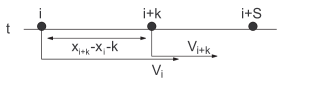
Figure 2: Collision-free condition between $i$-th and $i+k$-th car.

3 Metastable branches and their stability

Next, we investigate the fundamental diagram of this new hybrid model.

Figure 3: Fundamental diagram of the new Lagrange model. Parameters are set to $V_{max}=5$ and $S=2$, and the spatial period is 100 sites. The initial car density is varied from 0.05 to 0.95 in steps of 0.01. At each density, we start calculations from 30 randomly generated initial configurations, and show only the data at the time $t=100$. We observe several metastable branches in the deterministic case. The fluctuations of the branches show the fact that the asymptotic flow of the system sometimes becomes periodic instead of stationary between 0.2 $\leq\rho\leq$ 0.5.

In Fig. 3, we observe a complex phase transition from a free to congested state near the critical density 0.2 $\sim$ 0.4. There are many metastable branches in the diagram, similar to our previous models in Euler form [22, 23] or in other models with anticipation [24]. We also point out that there is a wide scattering area near the critical density in the observed data (Fig. 1) which may be related to these metastable branches. As we will discuss later, these branches may account for some aspects of the scattering area observed empirically.

First, we discuss properties of the state in the metastable branches. In all cases it consists of pairs of vehicles that move coherently with vanishing headway (see Fig. 4). Cars are represented by black squares, and the direction of the road is horizontal right and time axis is vertical down. The corresponding velocity distributions are also given in Fig. 5. We see that there are stopping cars which velocity are zero only in the case of the lowest branch given in the state in Fig. 4 (e).

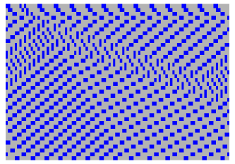
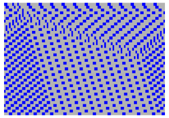
(a)                                   (b)

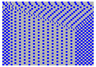
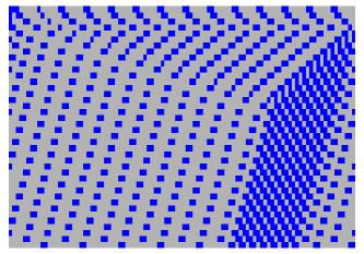
(c)                                   (d)

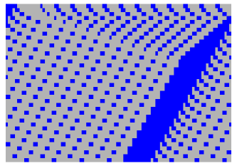
(e)

Figure 4: Spatio-temporal patterns of evolution of the uniform flow $\cdots 11000001100000\cdots$ at density $\rho=2/7$ with different strength of perturbation: (a) very weak, (b) less weak, (c) medium, (d) stronger and finally (e) strongest perturbation. The details of these perturbations are all explained in detail in the text. The stationary state of these five cases correspond to a state in each metastable branch appearing in Fig. 3, although the branch corresponding to (a) does not appear in the numerical simulations with random initial conditions.

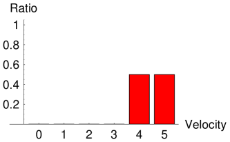
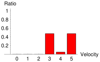
(a)                                   (b)

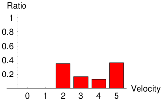
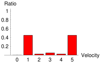
(c)                                   (d)

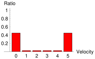
(e)

Figure 5: Velocity distributions in the case $\rho=2/7$, corresponding to the states given in fig. 4.

Next let us calculate the flow-density relation for each branch. In the metastable branches we find phase separation into a free-flow and a jamming region. In the former, pairs move with velocity $v_{f}$ and a headway of $d_{f}$ empty cells between consecutive pairs. In the jammed region, the velocity of the pairs is $v_{j}$ and the headway $d_{j}$. $N_{j}$ and $N_{f}$ are the numbers of cars in the jamming cluster and the free uniform flow, respectively. We assume $N_{f}$ and $N_{j}$ to be even so that there are $N_{f}/2$ and $N_{j}/2$ pairs, respectively. Then the total number of cars $N$ is given by $N=N_{j}+N_{f}$ and the total length of the system becomes $l=(d_{j}+2)N_{j}/2+(d_{f}+2)N_{f}/2$. Since the average velocity is $\bar{v}=(N_{f}v_{f}+N_{j}v_{j})/N$ and density and flow of the system are given by $\rho=N/l$ and $Q=\rho\bar{v}$, we obtain the flow-density relation as

$$Q=2\frac{v_{f}-v_{j}}{d_{f}-d_{j}}+\left(v_{j}-(d_{j}+2)\frac{v_{f}-v_{j}}{d_{f}-d_{j}}\right)\rho.\quad$$ (13)

From the stationary states in Fig. 4 we have

$$(a):(v_{f},v_{j},d_{f},d_{j})=(5,4,6,4)$$

$$(b):(v_{f},v_{j},d_{f},d_{j})=(5,3,7,3)$$

$$(c):(v_{f},v_{j},d_{f},d_{j})=(5,2,8,2)$$

$$(d):(v_{f},v_{j},d_{f},d_{j})=(5,1,9,1)$$

$$(e):(v_{f},v_{j},d_{f},d_{j})=(5,0,10,0)$$ (14)

Therefore the resulting equations for each branch are

$$Q=1+c\rho$$ (15)

where $c=1,1/2,0,-1/2,-1$, which correspond to the branches $A,B,C,D$ and $E$ in Fig. 6, respectively. End points of the branches are found to be given by $\rho_{1}=2/(d_{f}+2)$ and $\rho_{2}=2/(d_{j}+2)$, where $\rho_{1}$ is the point that the metastable branches intersect the free flow branch, and $\rho_{2}$ is the maximal possible density in the metastable branches. Note that all $\rho_{2}$ lie on the line $Q=-2\rho+2$, which is indicated as the broken line in Fig. 6.

Figure 6: A schematic diagram of the metastable branches ($A,B,C$ and $D$) and the jamming line ($E$) in the new model. The highest flow state is represented by $P_{0}$, which is quite unstable and easy to go down to the lower flow state $P_{A},\cdots,P_{E}$ according to the magnitude of the perturbation.

Next let us now study the stability of each metastable branch. We mainly consider the density $\rho=2/7$ and, in particular, we will focus on the uniform flow represented by $\cdots 11000001100000\cdots$, which shows the highest flow given in the point $P_{0}$ in Fig. 6.

Spatio-temporal patterns due to various kinds of perturbations are already seen in Fig. 4. Perturbation in this case means that some cars are shifted backwards at the initial configuration. The initial conditions for Fig. 4(a)-(e) are given as follows:

1. Very weak perturbation (one car is shifted one site backwards)$\cdots 11000010100000\cdots$

2. Weak perturbation (one car is shifted two sites backwards)$\cdots 11000100100000\cdots$

3. Moderate perturbation (one car is shifted three sites backwards)$\cdots 11001000100000\cdots$

4. Strong perturbation (one car is shifted five sites backwards)$\cdots 11100000100000\cdots$

5. Strongest perturbation (three cars are shifted backwards) $\cdots 11111000000000\cdots$

The stationary state of (a), (b), (c), (d) and (e) are given by the points $P_{A}$, $P_{B}$, $P_{C}$, $P_{D}$ and $P_{E}$ in Fig. 6, respectively. That is, if the system in $P_{0}$ is perturbated, then the flow easily goes down to a lower branch in the course of time depending on the magnitude of the perturbation. Since the density does not change due to the perturbation, we obtain $P_{A}:(2/7,9/7)$, $P_{B}:(2/7,8/7)$, $P_{C}:(2/7,1)$, $P_{D}:(2/7,6/7)$ and $P_{E}:(2/7,5/7)$ by substituting $\rho=2/7$ into eq. (15).

We see a jamming cluster propagating backwards in the cases of (d) and (e) in Fig. 4. In other cases the jamming cluster propagates forward ((a) and (b)) or does not move (c). These facts are related to the gradient of the metastable branches which are given by $c$ according to eq. (15).

4 Stochastic generalization

Finally we will combine the above model with the NS model in order to take into account the randomness of drivers. The NS model is written in Lagrange form as

$$x_{i}^{t+1}=x_{i}^{t}+\max\left\{0,\min\{V,x^{t}_{i+1}-x^{t}_{i}-1,x^{t}_{i}-x^{t-1}_{i}+1\}-\eta^{t}_{i}\right\}.$$ (16)

where $\eta^{t}_{i}=1$ with probability $p$ and $\eta^{t}_{i}=0$ with probability $1-p$. The last term in the mininum in (16) represents the acceleration of cars. The randomness in this model is considered as a kind of random braking effect, which is known to be responsible for spontaneous jam formation often observed in real traffic [2]. We also consider random accerelation in this model which is not taken into account in the NS model.

Thus a stochastic generalization of the hybrid model in the case of $S=2$ is similarly given by the following set of rules:

1. Random accerelation

   $$v^{(1)}_{i}=\min\{V_{max},v^{(0)}_{i}+\eta_{a}\}.$$ (17)

   where $\eta_{a}=1$ with the probability $p_{a}$ and $\eta_{a}=0$ with $1-p_{a}$.
   

2. Slow-to-accelerate effect

   $$v^{(2)}_{i}=\min\{v^{(1)}_{i},x^{t-1}_{i+S}-x^{t-1}_{i}-S\}.$$ (18)

3. Deceleration due to other vehicles

   $$v^{(3)}_{i}=\min\{v^{(2)}_{i},x^{t}_{i+S}-x^{t}_{i}-S\}.$$ (19)

4. Random braking

   $$v^{(4)}_{i}=\max\{v^{(3)}_{i}-\eta_{b},0\}$$ (20)

   where $\eta_{b}=1$ with the probability $p_{b}$ and $\eta_{b}=0$ with $1-p_{b}$.
   

5. Avoidance of collision

   $$v^{(n+1)}_{i} = \min\{v^{(n)}_{i},x^{t}_{i+1}-x^{t}_{i}-1+v^{(n)}_{i+1}\}$$ (21)

   with $n\geq 4$, which is an iterative equation that has to be applied until $v$ converges to $v^{(n+1)}_{i}=v^{(n)}_{i}(\equiv v_{i})$.
   

6. Vehicle movement

   $$x_{i}^{t+1}=x_{i}^{t}+v_{i}.$$ (22)

Again the velocity $v_{i}$ is used as $v^{(0)}_{i}$ in the next time step. Step 5 must be applied to each car iteratively until its velocity does not change any more, which ensures that this model is free from collisions. This is the difference between the deterministic and stochastic case. In the deterministic model it is sufficient to apply the avoidance of collision stage only once in each update, while in the stochastic case generically it has to be applied a few times in order to avoid collisions between successive cars.

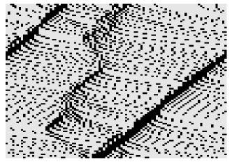
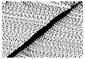
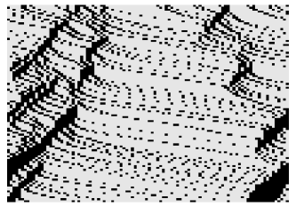
Figure 7: Fundamental diagrams and typical spatio-temporal patterns of the new stochastic model with different value of random parameters. Parameters are set to $V_{max}=5$ and $S=2$. Upper two figures are the case of $p_{a}=0$ and $p_{b}=0.2$, middle ones are $p_{a}=0.8$ and $p_{b}=0$, and the bottom ones are $p_{a}=0.8$ and $p_{b}=0.2$.

The fundamental diagrams of this stochastic model for some values of $p_{a}$ and $p_{b}$ are given in Fig. 7. The randomization effect can be considered as a sort of perturbation to the deterministic model. Hence some unstable branches seen in the deterministic case disappear in the stochastic case, especially if we consider the random braking effect as seen in Fig. 7. Random accerelation itself does not significantly destroy the metastable branches. Moreover, from the spatio-temporal pattern it is found that spontaneous jam formation is observed only if we allow random braking. Random accerelation alone is not sufficient to produce spontaneous jamming. We also note that a wider scattering area appears if we introduce both random accerelation and braking.

5 Concluding discussions

In this paper we have proposed a new hybrid model of traffic flow of Lagrange type which is a combination of the BCA and the s2s model. Its stochastic extension is also proposed by further incorporating stochastic elements of the NS model and random accerelation. The model shows several metastable branches around the critical density in its fundamental diagram. The upper branches are unstable and will decrease its flow under perturbations. It is shown that the magnitude of a perturbation determines the final value of flow in the stationary state. Moreover, introduction of stochasticity in the model makes the metastable branches dilute and hence produces a wide scattering area in the fundamental diagram. We would like to point out that this metastable region around the phase transition density is similar to so-called synchronized flow proposed by [25]. Our investigation shows that one possible origin of such a region is the occurance of many intermediate congested states near the critical density. If some of them are unstable due to perturbation or randomness, then a dense scattering area near the critical density is formed around the metastable branches. This is in some sense in between the two cases of a fundamental diagram based approach (with unique flow-density relation) and the so-called 3-phase model of [26] which exhibits a full two-dimensional region of allowed states even in the deterministic limit.

References

References

- [1] D. Helbing and H. J. Herrmann and M. Schreckenberg and D. E. Wolf (eds.), ”Traffic and Granular Flow ’99”, (Springer, 2000, Berlin).
- [2] D. Chowdhury, L. Santen and A. Schadschneider, Phys. Rep. 329 (2000) 199.
- [3] D. Helbing, Rev. Mod. Phys., 73 (2001) 1067.
- [4] S. Wolfram, Theory and applications of cellular automata, (World Scientific, 1986, Singapore).
- [5] B. Chopard and M. Droz, Cellular Automata Modeling of Physical Systems, (Cambridge University Press, 1998).
- [6] S. Bandini, R. Serra and F. S. Liverani (eds.), Cellular Automata: Research Towards Industry, (Springer, 1998).
- [7] M. Fukui and Y. Ishibashi, J. Phys. Soc. Jpn. 65 (1996) 1868.
- [8] K. Nagel and M. Schreckenberg, J. Phys. I France 2 (1992) 2221.
- [9] K. Nishinari and D. Takahashi, J. Phys. A. 31 (1998) 5439.
- [10] T. Tokihiro, D. Takahashi, J. Matsukidaira, and J. Satsuma, Phys. Rev. Lett. 76 (1996) 3247.
- [11] T. Musya and H. Higuchi, J. Phys. Soc. Jpn. 17 (1978) 811.
- [12] K. Nishinari, J. Phys. A 34 (2001) 10727.
- [13] J. Matsukidaira and K. Nishinari, Phys. Rev. Lett. 90 (2003) 088701.
- [14] K. Nishinari and D. Takahashi, J. Phys. A 33 (2000) 7709.
- [15] M. Takayasu and H. Takayasu, Fractals 1 (1993) 860.
- [16] S.C. Benjamin and N.F. Johnson, J. Phys. A 29 (1996) 3119.
- [17] A. Schadschneider and M. Schreckenberg, Ann. Physik 6 (1997) 541.
- [18] R. Barlovic, L. Santen, A. Schadschneider, and M. Schreckenberg, Eur. Phys. J. 5 (1998) 793.
- [19] M. Schreckenberg, A. Schadschneider, K. Nagel, and N. Ito, Phys. Rev. E 51 (1995) 2939.
- [20] K. Nishinari and M. Hayashi, Traffic statistics in Tomei express way, (The Mathematical Society of Traffic Flow, 1999, Nagoya).
- [21] M. Treiber, A. Hennecke and D. Helbing, Phys. Rev. E, 62 (2000) 1805.
- [22] K. Nishinari and D. Takahashi, J. Phys. A., 32 (1999) 93.
- [23] M. Fukui, K. Nishinari and D. Takahashi and Y. Ishibashi, Physica A, 303 (2002) 226.
- [24] M.E. Larraga, J.A. del Rio and A. Schadschneider, (2003) cond-mat/0306531.
- [25] B. S. Kerner and H. Rehborn, Phys. Rev. E, 53 (1996) 1297.
- [26] B.S. Kerner, S.L. Klenov, and D.E. Wolf, J. Phys. A 35 (2002) 9971.