Distribution of the local density of states, reflection coefficient and Wigner delay time in absorbing ergodic systems at the point of chiral symmetry

Abstract

Employing the chiral Unitary Ensemble of random matrices we calculate the probability distribution of the local density of states for zero-dimensional (”quantum chaotic”) two-sublattice systems at the point of chiral symmetry $E=0$ and in the presence of uniform absorption. The obtained result can be used to find the distributions of the reflection coefficent and of the Wigner time delay for such systems.

Spectral and transport properties of quantum systems with chiral symmetries attracted a considerable attention recentlyBr ; Tit ; AM ; off ; rflux ; QCD ; TI ; EK . The systems of the discussed type are characterized by random Hamiltonians of the form:

$${\cal H}_{ch}=\left(\begin{array}[]{cc}0&\hat{H}\\ \hat{H}^{\dagger}&0\end{array}\right)$$ (1)

serving to describe various physical situations, e.g. lattice systems with bond disorder of pure nearest-neighbour hopping typeBr ; Tit ; AM ; off , random magnetic flux models appearing in the context of the Quantum Hall effectrflux , as well as lattice QCD modelsQCD . Many other interesting examples can be found in the cited literature.

Replacing the block $\hat{H}$ in Eq.(1) with random rectangular matrices of the size $N_{A}\times N_{B}$ with independent, Gaussian-distributed complex entries we arrive at the object known as the chiral Gaussian Unitary Ensemble (chGUE)AZ . In the language of the two-sublattice disordered lattice system this model is known to correspond to the so-called universal ergodic (or ”zero-dimensional”, or ”quantum dot”) limit adequate if we are interested in energies smaller than the so-called Thouless energy $E_{c}$. The latter requirement means that the time to diffusively propagate through the system is much shorter than $\hbar/\Delta$, with $\Delta$ standing for the mean level spacing in the relevant energy range. Spectral statistics of chGUE matrices is well-studied by various methods and many explicit results are availablech1 ; ch2 ; ch3 ; iv ; ch4 ; ch5 .

One of the most striking features of the spectra of chiral systems is a specific behaviour of the spectral characteristics at zero energy. In zero-dimensional chiral systems this specific behaviour is manifested, in particular, via vanishing of the mean eigenvalue density $\rho_{av}(E)$ at the middle of the band, $E=0$, as long as $N_{A}=N_{B}$. For $N_{A}\neq N_{B}$ there exist exactly $|N_{A}-N_{B}|$ zero eigenvalues. All nonzero eigenvalues for chiral models appear in pairs $\pm\lambda_{n}$, with the corresponding eigenvectors being $|w_{n}^{\pm}\rangle=\left(\begin{array}[]{c}{\bf u}_{n}\\ \pm{\bf v}_{n}\end{array}\right)$. Here ${\bf u}_{n}$ and ${\bf v}_{n}$ are eigenvectors of the Hermitian matrices $\hat{H}\hat{H}^{\dagger}$ and $\hat{H}^{\dagger}\hat{H}$, of the size $N_{A}\times N_{A}$ and $N_{B}\times N_{B}$, respectively. To ensure the orthonormality of the eigenvectors $\left\langle w_{m}^{\pm}|w_{n}^{\pm}\right\rangle=\delta_{mn}$ we choose the normalisation ${\bf v}^{\dagger}_{n}{\bf v}_{n}={\bf u}^{\dagger}_{n}{\bf u}_{n}=1/\sqrt{2}$.

We first assume, for simplicity, that the number of lattice sites in the two sublattices are equal: $N_{A}=N_{B}=N$ and define in a usual way the exact local density of states (LDOS) at a site $j_{A}=1,2,...,N$ of the sublattice $A$ via the relation:

$$\rho_{j_{A}}(E_{\eta})=\frac{1}{\pi}\mbox{Im}\langle j_{A}|\frac{1}{E_{\eta}-{\cal H}}|j_{A}\rangle$$ (2)

$$=\frac{2}{\pi}\mbox{Im}\sum_{n=1}^{N}|u_{n}(j)|^{2}\frac{E_{\eta}}{E^{2}_{\eta}-\lambda^{2}_{n}}$$ (3)

where $u_{n}(j)$ stands for $j-th$ component of the eigenvector ${\bf u}_{n}$. Here we assume that the energy $E_{\eta}=E-i\eta$ is complex, the parameter $\eta>0$ standing for the level broadening due to an absorption, i.e. uniform-in-space losses of the flux of particles in the sample. In particular, for the energy $E$ chosen precisely in the center of the spectrum (”the point of chiral symmetry”) the LDOS is given by the most simple expression:

$$\rho_{j,A}(\eta)=\frac{2}{\pi}\sum_{n=1}^{N}|u_{n}(j)|^{2}\frac{\eta}{\eta^{2}+\lambda^{2}_{n}}.$$ (4)

For the lattice sites of the sublattice $B$ the LDOS is given by the same formula, with ${\bf u}_{n}(j)$ replaced by ${\bf v}_{n}(j)$.

The above expression is a very convenient starting point for calculating the distribution function of the local DOS at the spectrum center. In doing this we employ the method suggested for GUE without chiral structure inGUE . Namely, we consider the generating function (the Laplace transform of the probability density) $P(t)=\left\langle e^{-t\rho_{j,A}}\right\rangle_{chGUE}$ where the angular brackets stand for the ensemble averaging. Using that the eigenvalues $\lambda_{n}$ are statistically independent of the eigenvectors ${\bf u}_{n},{\bf v}_{n}$, and the components of the latter vectors behave in the large $N$ limit like independent complex Gaussian variables with zero mean and variances $\left\langle|u_{n}(j)|^{2}\right\rangle_{chGUE}=\frac{1}{2N}$ one can first perform the ensemble average over eigenvectors. After simple manipulations one arrives at the following representation for the generating function:

$$P(t)=\left\langle\frac{\det{\left(\eta^{2}+\hat{H}\hat{H}^{\dagger}\right)}}{\det{\left(\tilde{\eta}^{2}+\hat{H}\hat{H}^{\dagger}\right)}}\right\rangle_{H}$$ (5)

where we denoted $\tilde{\eta}=\sqrt{\eta^{2}+\eta t/(\pi N)}$. In this way the problem of calculating the generating function in question is reduced to evaluating the ensemble average of the ratio of characteristic polynomials of the random matrices $\hat{H}\hat{H}^{\dagger}$. The latter object (and its generalisations) were intensively studied in the literature recently, see ch4 ; ch5 , and the result is readily available:

$$P(t)=\frac{\pi}{2}\left[\epsilon I_{1}(\epsilon)K_{0}\left(\sqrt{\epsilon(\epsilon+2t/\pi)}\right)\right.$$ (6)

$$\left.+\left(\sqrt{\epsilon(\epsilon+2t/\pi)}\right)K_{1}\left(\sqrt{\epsilon(\epsilon+2t/\pi)}\right)I_{0}(\epsilon)\right]$$

where we denoted $\epsilon=2N\eta$ and considered this parameter to be finite when performing the large-N limit. Here $I_{n}(z),K_{n}(z)$ stand for the modified Bessel and Macdonald functions of the order $n$, respectively. The distribution function ${\cal P}(\rho_{A})$ of the LDOS can be found by inverting the Laplace transform Eq.(6) with respect to $t$ and is given by:

$${\cal P}(\rho_{A})=\frac{\epsilon}{2\rho_{A}}e^{-\frac{\epsilon}{2}(\pi\rho_{A}+1/\pi\rho_{A})}\left[I_{1}(\epsilon)+\frac{1}{\pi\rho_{A}}I_{0}(\epsilon)\right]$$ (7)

Having the LDOS distribution at our disposal, we can further utilise it for obtaining distributions of varous physical quantities of much interest describing scattering of a quantum particle from the two-sublattice disordered sample. In doing this we follow the method suggested recently by the first author in my1 . Consider a particle injected into the site $j_{A}$ of the sublattice $A$ through a one-channel infinite lead perfectly coupled to the system. The scattering of such a particle from our absorptive sample is described by the scattering matrix $S_{jA}$ expressed in terms of the matrix elements of the resolvent associated with the chiral Hamiltonian ${\cal H}$:

$$S_{jA}(E_{\eta})=\frac{1-iG}{1+iG}\quad,\quad G=\pi\langle j_{A}|\frac{1}{E_{\eta}-{\cal H}}|j_{A}\rangle.$$ (8)

In this way the problem of investigating statistics of the scattering matrix amounts to that of the diagonal entry $G$ of the resolvent. For an arbitrary energy $E$ the variable $G$ is a complex quantity and one has therefore to know the joint probability density of its real and imaginary parts. However, at the point $E=0$ of chiral symmetry $G$ turns out to be purely imaginary and therefore just proportional to the LDOS, Eq.(4), whose distribution ${\cal P}(\rho_{A})$ was calculated above, Eq.(7). As a result we can calculate the distribution of the reflection coefficient $R_{jA}(\eta)=|S_{jA}(\eta)|^{2}$. Below we present the distribution of a related object $\tau=1-R_{jA}=4\pi\rho_{jA}/(1+\pi\rho_{jA})^{2}$ which, following my1 , we suggest to call the ”probability of no return” (PNR). This quantity has meaning of the quantum-mechanical probability for a particle entering the system via a given channel never exit back to the same channel. It is well-defined for a given realization of disorder and will therefore show sample-to-sample fluctuations. Let us stress that in the case $\eta=0$ of no internal dissipation $S-$matrix is unitary for any energy and PNR is vanishing identically. For a system with absorption the unitarity is violated, giving rise to a nontrivial statistics of $\tau$:

$${\cal P}(\tau)=\frac{\epsilon}{\tau\sqrt{1-\tau}}e^{-\epsilon\left(\frac{2}{\tau}-1\right)}\left[I_{1}(\epsilon)+\left(\frac{2}{\tau}-1\right)I_{0}(\epsilon)\right]$$ (9)

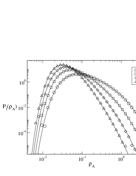
Figure 1: Numerical (symbols) and analytical (solid lines) results for the LDOS distribution of the sublattice $A$ for $\epsilon=1$, $N_{B}=300$ and $N_{A}=300-l,\;l=0,1,2,3$.

The above distribution can be further utilized for finding statistics of such interesting characteristic of quantum scattering as the so-called Wigner delay time $\tau_{W}=-i\partial S/\partial E$ intensively studied in recent years, see td1 ,td2 ,tsamp ,td3 and references therein. This can be done again following my1 , see also td3 . Indeed, remembering that nonzero values of $\tau$ arise solely due to an absorption, one can relate for small absorption the PNR value to the Wigner delay time by $\tau\simeq 2\epsilon\tau_{W}$td2 . Taking the corresponding limit in the distribution (9) we arrive at the distribution of the scaled variable $\tilde{\tau}_{W}=\tau_{W}/2N$:

$${\cal P}(\tilde{\tau}_{W})=\frac{1}{\tilde{\tau}^{2}_{W}}e^{-\frac{1}{\tilde{\tau}_{W}}}$$ (10)

The expression Eq.(10)) should be compared with the corresponding formula for the one perfect channel attached to an ergodic system modelled by GUE, i.e. without the chiral symmetry td1 : ${\cal P}(\tilde{\tau}_{W})=\frac{1}{\tilde{\tau}^{3}_{W}}e^{-\frac{1}{\tilde{\tau}_{W}}}$. The crossover between the two types of behavior is expected to happen in the present model with increasing energy parameter $E$ from zero to values much exceeding the mean level spacing. Investigating this interesting question requires however much more elaborate methods and is left for future research.

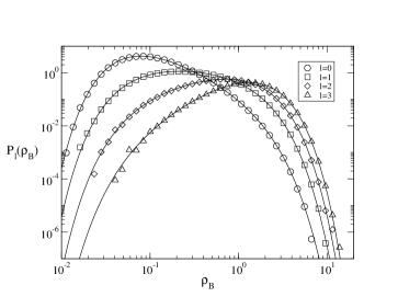
Figure 2: Numerical (symbols) and analytical (solid lines) results for the LDOS distribution of the sublattice $B$ for $\epsilon=1$, $N_{B}=300$ and $N_{A}=300-l,\;l=0,1,2,3$.

Let us now briefly discuss generalization of our results to the case of non-equivalent sublattices $N_{B}>N_{A}$. Note that in this case exactly $N_{B}-N_{A}=l$ zero modes are supported by the sublattice $B$, whereas only modes with nonzero eigenvalues give contribution to the LDOS for the sublattice $A$. Assuming that $l\ll N_{A},N_{B}$ one finds that LDOS distribution for the sites belonging to the sublattice $A$ is given by formula generalizing Eq.(7):

$${\cal P}_{l}(\rho_{A})=\frac{\epsilon}{2\pi^{l}\rho_{A}^{l+1}}e^{-\frac{\epsilon}{2}(\pi\rho_{A}+1/\pi\rho_{A})}\left[I_{l+1}(\epsilon)+\frac{1}{\pi\rho_{A}}I_{l}(\epsilon)\right]$$ (11)

whereas the LDOS distribution ${\cal P}_{l}(\rho_{B})$ for sites belonging to the sublattice $B$ is obtained from the above formula by replacing $l$ with $-l$. In Fig. (1) and Fig. (2) we compare this prediction with the results of direct numerical simulations of the random matrix Hamiltonian Eq.(1), for sublattices $A$ and $B$ correspondingly. It is instructive to compare the behavior of the mean LDOS for the two sublattices in the limit $\epsilon\to 0$:

$$\langle\rho_{A}\rangle=\frac{\epsilon}{2}\left[I_{l+1}(\epsilon)K_{l-1}(\epsilon)+I_{l}(\epsilon)K_{l}(\epsilon)\right]\to\frac{\epsilon}{4l}$$ (12)

$$\langle\rho_{B}\rangle=\frac{\epsilon}{2}\left[I_{l-1}(\epsilon)K_{l+1}(\epsilon)+I_{l}(\epsilon)K_{l}(\epsilon)\right]\to\frac{l}{\epsilon}$$ (13)

The singularity in the latter expression reflects presence of exactly $l$ zero modes supported by the sites of sublattice $B$.

After straightforward manipulations one can find that the distribution Eq.(9) is replaced by the following two formulas:

$${\cal P}_{l}(\tau_{A})=\frac{\epsilon}{\tau_{A}\sqrt{1-\tau_{A}}}e^{-\epsilon\left(\frac{2}{\tau_{A}}-1\right)}$$ (14)

$$\times\left[\left(v_{+}^{l}+v_{-}^{l}\right)I_{l+1}(\epsilon)+\left(v_{+}^{l+1}+v_{-}^{l+1}\right)I_{l}(\epsilon)\right],$$

$${\cal P}_{l}(\tau_{B})=\frac{\epsilon}{\tau_{B}\sqrt{1-\tau_{B}}}e^{-\epsilon\left(\frac{2}{\tau_{B}}-1\right)}$$ (15)

$$\times\left[\left(v_{+}^{l}+v_{-}^{l}\right)I_{l-1}(\epsilon)+\left(v_{+}^{l-1}+v_{-}^{l-1}\right)I_{l}(\epsilon)\right].$$

valid for the sublattices $A$ and $B$, respectively. Here the parameters $v_{+},v_{-}$ satisfy the conditions: $v_{+}v_{-}=1$ and $\frac{1}{2}(v_{+}+v_{-})=\left(\frac{2}{\tau_{A(B)}}-1\right)$. Finally, performing in Eq.(14) the limiting procedure discussed above, we arrive at the distribution of the (scaled) Wigner delay time $\tilde{\tau}_{W}$ for the one-channel lead attached to a site belonging to the $A-$ sublattice:

$${\cal P}_{l}(\tilde{\tau}_{W})=\frac{1}{l!}\frac{1}{\tilde{\tau}^{l+2}_{WA}}e^{-\frac{1}{\tilde{\tau}_{WA}}}$$ (16)

which generalizes the expression Eq.(10). In Fig. (3) we present the distribution of the Wigner delay times calculated numerically for various values of $l$ compared with this analytical result.

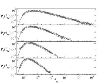
Figure 3: Numerical ($\circ$) and analytical (solid lines) results for the distribution of scaled Wigner delay times for sublattice $A$, for $\epsilon=1$, $N_{B}=300$ and $N_{A}=300-l,\;l=0,1,2,3$.

In fact, the time-delay distributions Eqs. (10) and (16) can be obtained in a more direct way. For this we notice that the expression Eq.(8) for the unitary scattering matrix $S_{A}(E)$ at real energies $E$ can be written in an equivalent form:

$$S_{A}(E)=\frac{\det{\left(E^{2}-iEP_{j_{A}}-\hat{H}\hat{H}^{\dagger}\right)}}{\det{\left(E^{2}+iEP_{j_{A}}-\hat{H}\hat{H}^{\dagger}\right)}}$$ (17)

where we used the $N_{A}\times N_{A}$ projection matrix $P_{j_{A}}=|j_{A}><j_{A}|$. Calculating now the Wigner delay time as the energy derivative of the logarithm of the above equation, and setting $E=0$ we arrive after straightforward manipulations to a simple formula:

$$\tau_{W}=2<j_{A}|\left(\hat{H}\hat{H}^{\dagger}\right)^{-1}|j_{A}>=2\sum_{n=1}^{N_{A}}\frac{|u_{n}(j_{A})|^{2}}{\lambda^{2}_{n}}$$ (18)

Comparison of this expression with Eq.(4) makes it clear that the Laplace transform $P(s)$ of the probability density for $\tilde{\tau_{W}}=\tau_{W}/2N_{A}$ can be obtained via the same manipulations as those leading to Eqs.(5) and (6). For the general case $0\leq l=N_{B}-N_{A}\ll N_{A},N_{B}$ we find:

$$P(s)=\left\langle\frac{\det{\left(\hat{H}\hat{H}^{\dagger}\right)}}{\det{\left(s/N^{2}_{A}+\hat{H}\hat{H}^{\dagger}\right)}}\right\rangle_{H}=\frac{2}{l!}s^{\frac{l+1}{2}}K_{l+1}(2\sqrt{s})$$

which can be immediately inverted yielding the distribution Eq.(16).

It is easy to repeat the same manipulations for the lead attached to a site of the larger sublattice $B$ and to find that Eq.(18) is replaced formally with

$$\tau_{W}=2<j_{B}|\left(\hat{H}^{\dagger}\hat{H}\right)^{-1}|j_{B}>$$ (19)

This expression, however, does not make any sense beyond the case $l=0$ of equivalent sublattices, since the corresponding $N_{B}\times N_{B}$ matrix $\hat{H}^{\dagger}\hat{H}$ is singular. We conclude therefore that the Wigner delay time at zero energy diverges for the sites belonging to the larger sublattice due to presence of zero modes.

In summary, we presented analytical as well as numerical results for the distribution of the local density of states for zero-dimensional chaotic system at the point of chiral symmetry $E=0$, and further utilized it for studying statistics of the reflection coefficient and Wigner delay times. Apart from investigating a gradual breakdown of the chiral symmetry with increasing energy parameter $E$ in ergodic systems, an interesting and challenging question is to study the LDOS fluctuations in chiral systems of higher dimensions. In particular, in disordered quantum wires the mean DOS is known to display a logarithmic singularityTit ; AM . It would be interesting to understand how that singularity affects the LDOS distribution, and how it is reflected in fluctuations of the related scattering characteristics.

YVF is grateful to LPTMS, Universite Paris-Sud for kind hospitality and financial support during initial stage of this work. Financial support by Brunel University VC grant (YVF) and by a grant from the German-Israeli Foundation for Scientific Research and Development (AO) is gratefully acknowledged.

References

- (1) [] On leave from Petersburg Nuclear Physics Institute RAS, 188350 Gatchina, Leningrad reg., Russia
- (2) P.W.Brouwer C.Mudry, B.D.Simons, and A.Altland Phys. Rev. Lett. 81 (1998) 862; Nucl.Phys.B 565 (2000) , 653;
- (3) P.W.Brouwer, C.Mudry and A. Furusaki Phys.Rev.Lett. 84 (2000), 2913; M. Titov, P.W.Brouwer, A. Furusaki and C.Mudry Phys. Rev. B 63 (2001) 235318
- (4) A.Altland and R.Merkt Nucl.Phys. B 607 (2001), 511
- (5) R.Gade Nucl.Phys.B 398 (1993), 499; A.Eilmes, R.A.Römer and M.Schreiber, Eur.Phys. J.B 1, (1998) 29
- (6) A. Altland and B.D.Simons J.Phys.A 32 (1999) L353; Nucl. Phys.B 562 (1999) 445; A. Furusaki Phys.Rev.Lett. 82 (1999) 604
- (7) For a review and further references see: J.J.M. Verbarschot and T.Wettig Annu.Rev.Nucl.Part.Sci. 50(2000) 343
- (8) K. Takahashi and S. Iida Phys. Rev. B63 (2001), 214201
- (9) S.N. Evangelou and D.E.Katsanos J.Phys.A 36 (2003), 3237
- (10) A.Altland and M.R.Zirnbauer Phys.Rev.B 55 (1997), 1142
- (11) J.J.M. Verbaarschot and I.Zahed Phys.Rev.Lett. 70 (1993), 3852; K. Slevin, T. Nagao Phys.Rev.B 50 (1994), 2380; P.J. Forrester Nucl.Phys.B 402 (1993), 709;
- (12) A.V.Andreev, B.D.Simons, N.Taniguchi Nucl.Phys.B 432 (1994) 487
- (13) A.D.Jackson, M.K. Sener, J.J.M. Verbaarschot Phys.Lett. B 387 (1996), 355; Nucl.Phys.B 479 (1996), 707; T.Guhr and T.Wettig J.Math.Phys. 37 (1996), 6395; Nucl.Phys.B 506 (1997), 589; R.A.Janik, M.A.Novak and I.Zahed Phys.Lett. B 392 (1997), 155; G. Akemann, P.H.Damgaard, U.Magnea and S.Nishigaki Nucl.Phys.B 487 (1997), 721
- (14) D.Dalmazi and J.J.M. Verbaarschot Nucl.Phys.B 592 (2001), 419; Y.V.Fyodorov Nucl.Phys.B 621 (2002), 643; Y.V.Fyodorov and E.Strahov Nucl.Phys.B 647 (2002), 581
- (15) D.A.Ivanov J.Math.Phys. 43 (2002), 126
- (16) Y.V.Fyodorov and G.Akemann JETP Lett. 77 (2003) 438 ; K.Splittorff and J.J.M. Verbaarschot Phys.Rev.Lett. 90(2003),041601
- (17) C.W.J. Beenakker, Phys.Rev.B 50, 15170 (1994); N.Taniguchi, V.N.Prigodin Phys.Rev.B 54, 14305 (1995)
- (18) Y.V.Fyodorov, JETP Letters 78, 250 (2003) [cond-mat/0304671]
- (19) Y.V. Fyodorov, H.-J. Sommers, J. Math. Phys. 38 (4), 1918 (1997); V.A.Gopar et al. Phys.Rev.Lett.77, 3005 (1996); P.W.Brouwer et al. Phys.Rev.Lett. 78, 4737 (1997);
- (20) C.W.J. Beenakker, P.W.Brouwer, Physica E 9, 463 (2001); S.A. Ramakrishna, N. Kumar, Phys. Rev.B 61, 3163 (2000)
- (21) T.Kottos, M.Weiss, Phys. Rev. Lett. 89, 056401 (2002); A. Ossipov et al. , Phys.Rev. B 61, 11411 (2000) and Europhys. Lett. 62, 719 (2003), T.Kottos, A. Ossipov and T. Geisel cond-mat/0307119
- (22) D.V.Savin, H.-J.Sommers Phys. Rev. E 68, 036211 (2003)