Hidden structure in the randomness of the prime number sequence?

Abstract

We report a rigorous theory to show the origin of the unexpected periodic behavior seen in the consecutive differences between prime numbers. We also check numerically our findings to ensure that they hold for finite sequences of primes, that would eventually appear in applications. Finally, our theory allows us to link with three different but important topics: the Hardy-Littlewood conjecture, the statistical mechanics of spin systems, and the celebrated Sierpinski fractal.

1 Introduction

Prime numbers have fascinated scientists of all times, and their history is closely related to the very history of Mathematics. Recently, the interest in prime numbers has received a new impulse because they have appeared in different contexts ranging from Cryptology [1] to Biology [2, 3] or quantum chaos [4, 5], where the fine structure in primes must reflect properties of very high Riemann zeros. But, despite the huge advances in number theory, many properties of the prime numbers are still unknown, and they appear to us as a random collection of numbers without much structure. In the last few years, some numerical investigations related with the statistical properties of the prime number sequence [7, 8, 6, 9] have revealed that, apparently, some regularity actually exists in the differences and increments (differences of differences) of consecutive prime numbers. For instance, some oscillations are found in the histogram of differences as we show in Fig. 1a. In that figure, one can see some spikes located at positions $6$, $12$, $18$, and so on. A similar behavior was reported by Kumar et al. [6], who showed that the histogram of increments has also a similar periodicity; in this case there are some grooves at increments given by $0$, $\pm 6$, $\pm 12$, etc (see Fig. 1b). These novel and promising findings have been thought to provide new information about the underlying unpredictable distribution of prime numbers and its potential applications.

The aim of this work is twofold: on the one hand we demonstrate that the apparent regularities observed by these authors do not reveal any structure in the sequence of primes, and that it is precisely a consequence of its randomness. On the other hand, we show that this randomness provides a new kind of predictable patterned behavior that we can characterize explicitly and compute analytically.

Figure 1: a) Histogram of differences for the first million of consecutive prime numbers. Filled black bars correspond to $6$, $12$, $18$,…b) Histogram of the increments (differences of differences). We have not plotted the negative part of the $x$ axis in b) to simplify comparison between both figures. In this work we are not concerned with the decreasing trend, but rather with the periodic oscillations observed.

The paper is organized as follows: first, we introduce a theoretical framework to calculate the properties of consecutive differences of prime numbers. After that, we check numerically the validity of the theory when finite sequences of primes are computed, and discuss some of the main results obtained. Finally, conclusions are summarized.

2 Theory

Essentially, we will be dealing with the sequences obtained from the primes by subtracting them iteratively. Our findings are based on two basic results: the first one is the fact that every prime $p>3$ is $p=\pm 1(\mod 6)$ (i.e., there exists an integer $N$ such that $p=6N\pm 1$); the second one, a theorem by Dirichlet which states that, for any pair of numbers $a$ and $q$ with no common divisors, there are infinitely many primes $p=a(\mod q)$. In addition, these primes are roughly equidistributed for each possible value of $a$ [10]. Setting $q=6$ this means that $p=+1(\mod 6)$ and $p=-1(\mod 6)$ equally likely. In a probabilistic language, if $P_{n}(+1)$ denotes the fraction of primes $p\leq n$ which are $+1(\mod 6)$ (hence $P_{n}(-1)=1-P_{n}(+1)$), then

$$\lim_{n\rightarrow\infty}P_{n}(\pm 1)=\frac{1}{2},$$ (1)

Despite the apparent lack of structure that this result suggests, the numerical results concerning differences between primes cited above inspired us to search for regularities in the sea of randomness of the prime number sequence.

Now, we build the sequence of differences of consecutive primes, $D^{(1)}$, the sequence of differences of consecutive differences, $D^{(2)}$ and, in general, the m-differences, $D^{(m)}$, defined as differences of consecutive (m-1)-differences. For instance, taking the sequence of primes greater than $3$: $5$, $7$, $11$, $13$, $17$, $19$, $23$, $29$, $31$, $37$,…, we find:

$$D^{(1)} = 2,4,2,4,2,4,6,2,6,\ldots,$$ (2)

$$D^{(2)} = 2,-2,2,-2,2,2,-4,4,\ldots.$$ (3)

Note that all numbers are even because all primes $p\geq 3$ are odd.

The structure of these m-differences becomes clearer when we write them modulo 6 (this choice will be clarified below). Hereafter, we will term $d^{(m)}$ the integer between $-2$ and $2$ such that $d^{(m)}=D^{(m)}(\mod 6)$. As all the numbers in the sequences given by Eqs. (2)-(3) are even, $d^{(m)}$ can only take the values $0$ and $\pm 2$. At this point, the reader will have noted that the origin of the periodicity seen in the histograms of differences is a consequence of the fact that every prime number is $\pm 1(\mod 6)$. More explictly, we will find a $0$ in the $d^{(1)}$ sequence whenever two consecutive primes are both of the type $+1$ or both $-1$. Conversely, we will find $+2$ (respectively $-2$) only when consecutive primes are $-1$ and $+1$ ($+1$ and $-1$). Then, given equation (1), the probability of finding a $0$ in the sequence is twice that of finding $+2$ or $-2$. We want to remark that we have made the only extra assumption that consecutive primes can be $\pm 1$ independently, that is, the correlations between consecutive primes are negligible. Nevertheless, this is a hypothesis that we expect to hold for very large sequences of primes (average correlations will disappear for long enough sequences), but that we can not prove: this makes all our work a kind of conjecture, or only an approximation. Note that, if we consider the prime numbers to be $+1$ or $-1$ independently, taking the sequence in order (consecutive primes) makes no difference with considering differences between any pair of given primes, even if they are not consecutive.

In the same way, we can rate the relative frequencies for the $d^{(2)}$ sequence, noting that the terms we are subtracting are not $\pm 1$, but $0$ and $\pm 2$. Therefore, the frequency of an outcome to be $0$ is $2/3$ times that of the frequencies to be $+2$ or $-2$. This corresponds to the grooves in the histogram of increments in Fig. 1b.

At this point, we can calculate iteratively the subsequent frequencies for any m-difference. Nevertheless, we provide an exact formula to calculate them at any order through the generating function of the $d^{(m)}$ sequences. This task can be achieved because the m-differences satisfy some recurrence relations for a given piece of $m+1$ prime numbers. Let $s_{0}\ldots s_{m}$ denote the value of those primes modulo $6$, then:

$$d^{(m)}(s_{0},\ldots,s_{m})=\sum_{k=0}^{m}\left(\begin{array}[]{c}m\\ k\end{array}\right)(-1)^{k}s_{k}.$$ (4)

So our search for $0$ (respectively $+2$ and $-2$) in the sequences requires counting the number of solutions to the equation $d^{(m)}=0$ ($=+2$ and $=-2$). For a probability distribution $p_{t}$ of a discrete variable $t$, we can define a generating function [11]:

$$G(z)=\sum_{t}p_{t}z^{t}.$$ (5)

The probability distribution in which we are interested is $P^{t}(m)$, which is the probability that a given sequence of $m+1$ consecutive primes has an $m$-difference $d^{(m)}=t$, where $t$ can only take values $0$, $2$ and $-2$. It’s associated generating function is:

$$G_{m}(z)=P^{0}(m)+P^{2}(m)z^{2}+P^{-2}(m)z^{-2}.$$ (6)

We have made the assumption that the $s_{i}$ in a sequence $(s_{0},\ldots,s_{m})$ are all independent, so the probabilities $P^{t}(m)$ are proportional to the number of sequences such that $d^{(m)}(s_{0},\ldots,s_{m})=t$. Using this, we can write the generating function in (6) (forgetting the factor $2^{-(m+1)}$, which accounts for the total number of different sequences $(s_{0},\ldots,s_{m})$) as:

$$G_{m}(z)=\sum_{s_{0}=\pm 1}\ldots\sum_{s_{m}=\pm 1}\left\{z^{d^{(m)}}\delta(d^{(m)}-0)+z^{d^{(m)}}\delta(d^{(m)}-2)+z^{d^{(m)}}\delta(d^{(m)}+2)\right\},$$ (7)

which using $\delta(d^{(m)}-0)+\delta(d^{(m)}-2)+\delta(d^{(m)}+2)=1$ turns to be:

$$G_{m}(z)=\sum_{s_{0}=\pm 1}\ldots\sum_{s_{m}=\pm 1}z^{d^{(m)}}.$$ (8)

This function has some interesting properties. For instance, $G_{m}(1)=2^{m+1}$ provides all the possible sequences of primes that we need to evaluate to determine the relative frequencies of $0$ and $\pm 2$. Similarly, $\frac{1}{6}\sum_{n=0}^{5}G_{m}(e^{n\pi i/3})$ gives us only those combinations of primes for which $d^{(m)}=0$. In other words,

Figure 2: Relative frequency of appearing $P_{0}(m)$ for the first $m=1000$ m-differences. Note that it displays a quasi-periodic behavior with $m$.

it helps us to calculate (performing the sums) the relative frequency of zeroes in the m-difference sequence, $P^{0}(m)$ as

$$P^{0}(m)=\frac{1}{3}\left(1+\prod_{k=0}^{m}\cos\left[\frac{\pi}{3}\left(\begin{array}[]{c}m\\ k\end{array}\right)\right]+\prod_{k=0}^{m}\cos\left[\frac{2\pi}{3}\left(\begin{array}[]{c}m\\ k\end{array}\right)\right]\right).$$ (9)

Using a similar argument it can be shown that $P^{+2}(m)=P^{-2}(m)=(1-P^{0}(m))/2$. Fig. 2 shows $P^{0}(m)$ for the first $m=1000$ m-differences.

Figure 3: Pascal’s triangle modulo 3: we take the numerical triangle where the small black triangles are placed at those values that are non-zero ($\mod 3$). The resulting figure belongs to the family of Sierpinski’s gaskets. Solid arrows show the empty rows (except the first and last element) that give maxima for $m$ in Fig. 2. Dashed arrows show empty rows except for the central element: they give the position of the minima.

The quasi-periodic behavior displayed by $P^{0}(m)$ is also remarkable. This behavior arises from the properties of the binomial coefficients appearing in equation (9) and the periodicity of the cosine. Thus, a maximum of $P^{0}(m)$ is found whenever all the elements in a row of Pascal’s triangle (except the first and the last, which are always $1$) are multiples of $3$. So, the maxima are located at $m=3^{n}$ and the minima at $m=2\cdot 3^{n}$, where $n=0,1,2,\ldots$ These maxima and minima can be easily identified graphically in Fig. 3, which represents a kind of Sierpinski’s gasket obtained from the modulo $3$ Pascal’s triangle. We want to stress that this is an analytical result, and that the correspondence between the properties of $P^{0}(m)$ and Pascal’s triangle can be shown to be rigorously deduced from the properties of the binomial coefficients.

A connection can be found between our ideas and a classical number theory conjecture due to Hardy and Littlewood [12] which states:

Conjecture 1 (Hardy and Littlewood)

Let $b_{0},b_{1},\ldots,b_{m}$ be $m$ distinct integers, and $P(x;b_{0},b_{1},\ldots,b_{m})$ the number of groups $n+b_{0},n+b_{1},\ldots,n+b_{m}$ between $1$ and $x$ consisting wholly of primes. Then

$$\lim_{x\to\infty}P(x)\sim G(b_{0},b_{1},\ldots,b_{m})\int_{2}^{x}\frac{\textrm{d}x^{\prime}}{(\ln x^{\prime})^{m+1}},$$ (10)

where

$$G(b_{0},b_{1},\ldots,b_{m})=\prod_{p\geq 2}\left(\left(\frac{p}{p-1}\right)^{m}\frac{p-\nu}{p-1}\right),$$ (11)

$\nu=\nu(p;b_{0},b_{1},\ldots,b_{m})$ is the number of distinct residues of $b_{0},b_{1},\ldots,b_{m}$ to modulus $p$, $p$ are the prime numbers and $n$ is a natural number.

Formula (11) can be rewritten using that:

$$G(b_{0},b_{1},\ldots,b_{m})=C_{m}H(b_{0},b_{1},\ldots,b_{m}),$$ (12)

where

$$C_{m}=\prod_{p>(m+1)}\left(\left(\frac{p}{p-1}\right)^{m}\frac{p-1-m}{p-1}\right),$$ (13)

$$H(b_{0},b_{1},\ldots,b_{m})=\prod_{p\leq(m+1)}\left(\left(\frac{p}{p-1}\right)^{m}\frac{p-\nu}{p-1}\right)\prod_{p|\Delta,p>(m+1)}\left(\frac{p-\nu}{p-1-m}\right),$$ (14)

and $\Delta$ is the product of the differences of the $b$’s. By $p|\Delta$ we mean that $\Delta$ is divisible by $p$, $C_{m}$ are known as the Hardy-Littlewood constants. Written in this form, all the dependence of $G$ on the actual members of the group of primes is contained in $H$. But $H$ is a finite expression, and in principle can be evaluated for all cases of interest. Moreover, as for fixed length $m$ of a group of primes the other terms of $G$ are identical, the different frequency of appearance of each type of groups of the same length depends only on $H$. Note that this conjecture does not use that the primes $n+b_{0},n+b_{1},\ldots,n+b_{m}$ have to be consecutive, in that sense, it has no relationship with our results. But we have already said that our results should hold also for non consecutive primes, due to the fact that they are only based in considering independent occurrences of $+1$ and $-1$ primes. So we could try to use the Hardy-Littlewood conjecture to compute the relative frequency of different groups of primes. We are interested in what we have called m-differences. A set of $n+b_{0},n+b_{1},\ldots,n+b_{m}$ differences between primes defines a m-difference of order $m$ and value:

$$D^{(m)}(b_{0},\ldots,b_{m})=\sum_{k=1}^{m}\left(\begin{array}[]{c}m\\ k-1\end{array}\right)(-1)^{k-1}b_{k}.$$ (15)

Again, we denote $d^{(m)}=D^{(m)}(\mod 6)$. The relative frequency of appearances of a given value $0$, $+2$ or $-2$ of $d^{(m)}$ for a constant $m$ is proportional to all the sets $(b_{0},\ldots,b_{m})$ that produce that value of $d^{(m)}$, and from equations (10) and (12) the contribution of each set is proportional to $H(b_{0},\ldots,b_{m})$. We define then $\mathcal{H}^{t}(m)$ as the sum of all the $H(b_{0},\ldots,b_{m})$ such that $d^{(m)}(b_{0},\ldots,b_{m})=t$. This $\mathcal{H}^{t}(m)$ is proportional to the number of groups of consecutive primes $n+b_{0},n+b_{1},\ldots,n+b_{m}$ which have $d^{(m)}(b_{0},\ldots,b_{m})=t$, and hence is proportional to the probability $P^{t}(m)$ that a given m-difference has value $t(\mod 6)$.

Figure 4: Histogram of differences for the first million of consecutive prime numbers, divided by the factors $\prod_{p|\Delta}\frac{p-1}{p-2}$.

Using this, we can write:

$$P^{0}(m)\propto\mathcal{H}^{0}(m)=\sum_{\forall\textrm{set}{\bf b}\backslash d^{(m)}=0}H(b_{0},\ldots,b_{m})$$ (16)

$$P^{+2}(m)\propto\mathcal{H}^{+2}(m)=\sum_{\forall\textrm{set}{\bf b}\backslash d^{(m)}=+2}H(b_{0},\ldots,b_{m})$$ (17)

$$P^{-2}(m)\propto\mathcal{H}^{-2}(m)=\sum_{\forall\textrm{set}{\bf b}\backslash d^{(m)}=-2}H(b_{0},\ldots,b_{m})$$ (18)

From our results, we make the following conjecture concerning the sums of function $H$:

$$\mathcal{H}^{+2}(m)=\mathcal{H}^{-2}(m)\equiv\mathcal{H}^{2}(m),$$ (19)

and from it we make a final conjecture that relates explicitly our formula (9) with the Hardy-Littlewood theory:

$$P^{0}(m)=\frac{\mathcal{H}^{0}(m)}{\mathcal{H}^{0}(m)+2\mathcal{H}^{2}(m)}$$ (20)

We have found no way to perform the infinite sums in (16-18), but we find formula (20) a beautiful relation and an interesting open problem. This relation between our theory and the well established Hardy-Littlewood theory shows that we can extract some information in our theory directly from Hardy and Littlewood’s developments, and therefore giving further strength to our point. From equation (14) we can see, for instance, that for $m=1$ (differences between consecutive primes), the probability of finding a difference of value $\Delta$ is proportional to $\prod_{p|\Delta}\frac{p-1}{p-2}$. Hence, dividing the histogram a) of Fig. 1 by this factor, the periodicity disappears, as shown in Fig. 4. The case $m=1$ is specially simple because the factor $\nu$ is trivially 1, and $\Delta$ is just the value of the difference between primes. For higher $m$-differences the problem is harder, as we can no longer set $\nu$ and $\Delta$ just from the values of $m$ and the $m$-difference we are interested in: in this case, for each $\Delta$ it is necessary to find all the groups $(b_{0},\ldots,b_{m})$ from which it can be obtained, and compute the whole factor $H(b_{0},\ldots,b_{m})$ associated with them. Our theory establishes a connection between the local properties (in the sense that they only apply to single groups $(b_{0},\ldots,b_{m})$) in the Hardy-Littlewood theory and global properties we describe, namely the $m$-differences, which depend on all the possible groups $(b_{0},\ldots,b_{m})$. It gives, through equation (9), a prediction that is easily computed for any $m$, while from Hardy and Littlewood’s results it is very difficult to say anything beyond $m=1$.

3 Numerical Results and Discussion

All the theoretical results presented in Sec. II stand if we consider the infinite sequence of primes. Now we consider the situation in which we pick a finite sequence of primes. In such a case, we expect some deviations from the results presented above due to, for instance, the transient behavior known as Chebyshev’s bias. Chebyshev noted that at the beginning of the sequence there are more primes of type $-1$ than of type $+1$. Moreover, Bays and Hudson [14] proved that the first time when $P_{n}(+1)>P_{n}(-1)$ occurs for $n=608,981,813,029$. This huge number is of the order of magnitude of $10^{13}$, bigger than $2^{39}$ and higher than numbers used for usual calculations without using specialized software. Nevertheless, this is a misleading result because the relative error of considering that $P_{n}(+1)=P_{n}(-1)=1/2$ is about $1.6\%$ for the first $1,000$ primes, about $0.2\%$ for the first $10,000$ and just $0.08\%$ for the first $100,000$. This relative error continues to decrease for increasing number of primes, so any finite sequence will reproduce our predictions with enough accuracy. Moreover, from the work of Littlewood [15] it is now well known that the inequality $P_{n}(-1)>P_{n}(+1)$ is reversed for infinitely many integers.

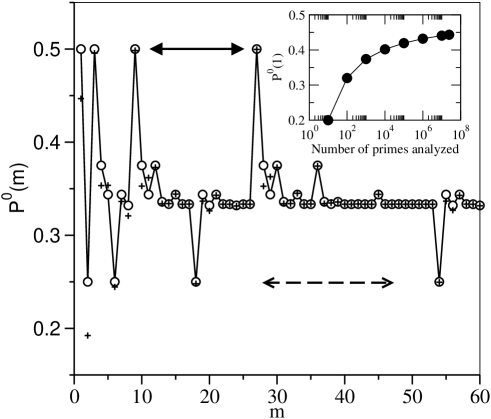
Figure 5: Relative frequency of appearing $P_{0}(m)$ for the first $m=60$ m-differences. Circles stand for the theoretical value and pluses for the value obtained computing such m-differences for all the primes lower than $2^{31}$. The arrows show more clearly the position of the maxima and minima exposed at Fig. 3. Inset: numerical values of $P_{0}(1)$ as a function of the length of the sequence analyzed. Although slow, the convergence to the exact value ($0.5$) is monotonous.

In Fig. 5 we show both theory and numerics. As we anticipated, there are some slight deviations but just at a small number of points. We have checked that these deviations reduce monotonously as we take larger sequences, due to the vanishing of Chebyshev’s bias as we increase the sequence size (see inset in Fig. 5). One criticism may be that the error is significantly large in some cases, but note that this error is not large enough to hide the periodicity in the sequences. For instance, for one of the worst cases, $m=1$, we predicted $P^{0}(1)=2P^{\pm 2}(1)$ but, actually, we have found numerically $P^{0}(1)=1.62P^{\pm 2}(1)$. Thus, the periodicity modulo $6$ is still transparent in spite of the fact that its strength deviates from the predicted one.

The reason why we use $6$ is that it is the first factor giving non-trivial information about the prime numbers. The first number to give us information about them is 2: it says that the rest of the primes cannot be multiples of 2. The same applies for 3. 4 gives no new information, as it is $4=2^{2}$, so it only says that prime numbers cannot be multiple of 2. 5, of course, excludes its own multiples. 6 is the first product of two different primes, and hence, saying that the prime numbers are of the form $6n\pm 1$ says that they cannot be multiples of 2 nor multiples of 3. From this simple observation, the fact that $m$-differences have to be $0(\mod 6)$ or $\pm 2(\mod 6)$ is readily derived. If we tried to repeat the same formalism with 4, we should see that all the primes are $4n\pm 1$, which is the same as saying that they are $1(\mod 2)$, that is, odd numbers. $m$-differences would be $0(\mod 4)$ or $\pm 2(\mod 4)$. But it has no sense considering this difference of sign between $+2(\mod 4)$ and $-2(\mod 4)$, as both things are exactly the same. So we would only be able to talk about $0(\mod 4)$ and $2(\mod 4)$, which means that both of them are equiprobable, and so no periodicity with period 4 should be observed, as in fact happens. Our results can be generalized taking other divisors $q$ instead of $6$. As 6 is $2\times 3$ and thus has non-trivial information about the sequence of prime numbers, the same happens with all the different products of primes. That is, our formalism can be extended to $2\times 5=10,2\times 7=14,2\times 11=22,2\times 13=26,2\times 3\times 5=30$, etc., predicting secondary periodicities in the $m$-differences histograms. This periodicities have already been observed in references [7, 8], and are explained in the framework of our theory.

Moreover, we may also consider the case in which the differences are evaluated between non-consecutive primes provided that they are picked at random. The results will remain the same because all the differences are calculated modulo $6$. For instance, a chaotic system with energy levels proportional to prime numbers will display oscillations in the spectrum of the emitted light through radiative transitions, because the frequency of the emitted light is proportional to the difference between energy levels (consecutive or not).

Another observation that supports our findings is the jumping champion phenomenon: at the beginning of the prime numbers sequence, the most often occurring 1-difference is 6. From $10^{35}$ it is 30, and there is evidence that from around $10^{450}$ it is 210, etc. In reference [16] this phenomenon, also related with the Hardy-Littlewood conjecture, is studied in detail. Table 3 in this reference shows histograms of gaps between consecutive primes for primes next to $10^{30}$, $10^{40}$, $10^{400}$ and $10^{450}$. Although statistics is not good enough in the biggest cases, in all of them the periodicity of period 6 is clearly displayed, giving a numerical evidence of our findings far beyond our own numerical calculations. Note also that all the known jumping champions are multiples of 6, as should be expected.

Finally, we can reformulate all the presented findings referring to the fact that the random structure of the $\pm 1$ primes resembles the high temperature (disordered) phase of spin systems [17]. This analogy can be cast explicitly by means of the Hamiltonian

$${\mathcal{H}}\equiv d^{(m)}(s_{0},\ldots,s_{m})=\sum_{k=0}^{m}\left(\begin{array}[]{c}m\\ k\end{array}\right)(-1)^{k}s_{k}.$$ (21)

Then, the generating function $G_{m}(z)$ is equal to the partition function of ${\mathcal{H}}$, ${\mathcal{Z}}$, if we identify the temperature as $k_{B}T=-1/\log z$. Note that this would correspond to a spin system defined on a one dimensional lattice without interactions between spins and subjected to an applied external field

$$B_{k}=\left(\begin{array}[]{c}m\\ k\end{array}\right)(-1)^{k}.$$ (22)

Likewise, we could take some advantage of the collected knowledge in spin systems to gain some insight into the properties of the products between primes. These products are the basis of some encrypting systems [1]. For instance, let us consider an interacting Hamiltonian of the form

$${\mathcal{H}}=\sum_{i,j}J_{ij}s_{i}s_{j}.$$ (23)

where the coupling constants $J_{ij}$ would depend on the recurrence relations between sequences of products. We expect this kind of approach to hold because the product of two primes will also be of the form $\pm 1(\mod 6)$.

4 Conclusions

We have studied the general behavior of consecutive differences between primes, both theoretically and numerically. Our theoretical predictions are based on a theorem by Dirichlet and on a hypothesis that neglects a kind of correlations between prime numbers. In principle they are only valid for the whole sequence of primes, but we find that they are also accurate for finite sequences. The deviations found are due to the transient behavior known as Chebyshev’s bias. Furthermore, the theory is still valid if the differences are computed between non-consecutive primes, and Chebyshev’s bias will be less pronounced.

Our main conclusion is that the main feature of the sequence of prime numbers, namely, its randomness, hides an underlying behavior arising when successive differences are computed. Thus, new and interesting phenomena can be derived and novel applications can be settled. For instance, the length of the periodic orbits in quantum chaos is related to the zeroes of Riemann’s function and these with the prime numbers [5]. So, these new findings can be of interest in the study of their statistical properties and engage with random matrix theory and the most outstanding problem in number theory: Riemann’s hypothesis [4]. We have related our theory to established number theory through the Hardy-Littlewood conjecture. We have also found a connection between our theory and the statistical mechanics of spin systems.

To conclude, we mention another interesting example in which the differences between primes are crucial, which is related to the fact that the life cycles of different animal species are precisely prime numbers. In this case, the life or death of the species depends on this property [2].

References

- [1] M. Stallings, Cryptography and network security: principles and practice, (Prentice Hall, New Jersey, 1999)
- [2] E. Goles, O. Schulz and M. Markus, Complexity 6 (2001) 33.
- [3] J. Tohá and M. A. Soto, Medical Hypotheses 53(4) (1999) 361.
- [4] M. V. Berry, Inst. Phys. Conf. Ser. No. 133 (1993).
- [5] J. Sakhr, R. K. Bhaduri and B. P. van Zyl, Phys. Rev. E 68 (2003) 026206.
- [6] P. Kumar, P. C. Ivanov and H. E. Stanley, cond-mat/0303110 (2003).
- [7] M. Wolf, Proc. of the 8th Joint EPS-APS Int. Conf. Physics Computing’96, P. Borcherds et al, eds. (Kraköw, 1996) s. 361.
- [8] M. Wolf, Physica A 274 (1999) 149.
- [9] S. R. Dahmen, S. D. Prado and T. Stuermer-Daitx, Physica A 296 (2001) 523.
- [10] L. Dirichlet, König. Preuss. Akad. 34 (1837) 45. Reprinted in Dirichlets Werke, vol 1, (Reimer, Berlin and Chelsea, Bronx (NY), 1889–97 and 1969).
- [11] H. S. Wilf, Generating Functionalogy, 2nd ed. Academic Press, (New York, 1994).
- [12] G. H. Hardy and J. E. Littlewood, Acta Math. 44 (1923) 1.
- [13] I. Richards, Bull. Amer. Math. Soc. 80 (1974) 419.
- [14] C. Bays and R. H. Hudson, Math. Comp. 32 (1978) 571.
- [15] J. E. Littlewood, Comptes Rendus 158 (1914) 1869.
- [16] A. Odlyzko, M. Rubinstein and M. Wolf, Exp. Math. 8 (1999) 107.
- [17] K. Huang, Statistical Mechanics, 2nd ed. John Willey & Sons, (New York, 1987).