Time-Dependent Partition-Free Approach in Resonant Tunneling Systems
Abstract
An extended Keldysh formalism, well suited to properly take into account the initial correlations, is used in order to deal with the time-dependent current response of a resonant tunneling system. We use a partition-free approach by Cini in which the whole system is in equilibrium before an external bias is switched on. No fictitious partitions are used. Despite a more involved formulation, this partition-free approach has many appealing features being much closer to what is experimentally done. In particular, besides the steady-state responses one can also calculate physical dynamical responses. In the noninteracting case we clarify under what circumstances a steady-state current develops and compare our result with the one obtained in the partitioned scheme. We prove a Theorem of asymptotic Equivalence between the two schemes for arbitrary time-dependent disturbances. We also show that the steady-state current is independent of the history of the external perturbation (Memory Loss Theorem). In the so called wide-band limit an analytic result for the time-dependent current is obtained. In the interacting case we work out the lesser Green function in terms of the self energy and we recover a well known result in the long-time limit. In order to overcome the complications arising from a self energy which is nonlocal in time we propose an exact non-equilibrium Green function approach based on Time Dependent Density Functional Theory. The equations are no more difficult than an ordinary Mean Field treatment. We show how the scattering-state scheme by Lang follows from our formulation. An exact formula for the steady-state current of an arbitrary interacting resonant tunneling system is obtained. As an example the time-dependent current response is calculated in the Random Phase Approximation.
pacs:
05.60.Gg Quantum transport72.10.Bg General formulation of transport theory
85.30.Mn Junction breakdown and tunneling devices (including resonance tunneling devices)
I Introduction
A resonant tunneling system is essentially a mesoscopic region, typically a semiconductor heterostructure, coupled to two metallic leads, which play the role of charge reservoirs. In a real experiment the whole system is in thermodynamic equilibrium before the external disturbance is switched on and one can assign a unique temperature and chemical potential . Therefore, the initial density matrix is where is the total Hamiltonian and is the total number of particles. By applying a bias to the leads at a given time, charged particles will start to flow through the central device from one lead to the other. As far as the leads are treated as noninteracting, it is not obvious that in the long-time limit a steady-state current can ever develop. The reason behind the uncertainty is that the bias represents a large perturbation and, in the absence of dissipative effects, e.g., electron-electron or electron-phonon scatterings, the return of time-translational invariance is not granted.
An alternative approach to this quantum transport problem has been suggested by Caroli et al.caroli1 ; caroli2 who state: “It is usually considered that a description of the system as a whole does not permit the calculation of the current”.caroli1 Their approach is based on a fictitious partition where the left and right leads are treated as two isolated subsystems in the remote past. Then, one can fix a chemical potential and a temperature for each lead, . In this picture the initial density matrix is given by , where and now refer to the isolated lead. The current will flow through the system once the contacts between the device and the leads have been established. Hence, the time-dependent perturbation is a lead-device hopping rather than a local one-particle level-shift. Since the device is a mesoscopic object, it is reasonable to assume that the hopping perturbation does not alter the thermal equilibrium of the left and right charge reservoir and that a non-equilibrium steady state will eventually be reached. This argument is very strong and remains valid even for noninteracting leads. Actually, the partitioned approach by Caroli et al. was originally applied to a tight-binding modelcaroli1 describing a metal-insulator-metal tunneling junction and then extended to the case of free electrons subjected to an arbitrary one-body potential.caroli2 This extension was questioned by Feuchtwang;feuchtwang1 ; feuchtwang2 the controversy was about the appropriate choice of boundary conditions for the uncontacted-system Green functions. In later years the non-equilibrium Green function techniqueskb-book ; keldysh-jetp1965 in the partitioned approach framework were mainly applied to investigate steady-state situations. An important breakthrough in time-dependent non-equilibrium transport was achieved by Wingreen et al.wingreen ; jauho ; jauhocond ; haug Still in the framework of the partitioned approach, they derive an expression for the fully nonlinear, time-dependent current in terms of the Green functions of the mesoscopic region (this embedding procedure holds only for noninteracting leads). Under the physical assumption that the initial correlations are washed out in the long-time limit, their formula is well suited to study the response to external time-dependent voltages and contacts.
The limitations of the partitioned approach are essentially three. First, it is difficult to partition the electron-electron interactions between the leads and between the leads and the device. These interactions are important for establishing dipole layers and charge transfers which shape the potential landscape in the device region. Second, there is a crucial assumption of equivalence between the long-time behavior of the 1) initially partitioned and biased system once the coupling between the subsystems is established and 2) the whole partition-free system in thermal equilibrium once the bias is established. Third, the transient current has no direct physical interpretation since in a real experiment one switches on the bias and not the contacts; moreover, there is no well defined prescription which fixes the initial equilibrium distribution of the isolated central device.
In this paper we use a partition-free scheme without the above limitations. This conceptually different time-dependent approach has been proposed by Cini.cini He developed the general theory for the case of free electrons described in terms of a discrete set of states and a continuum set of states with focus on semiconductor junction devices. For a one-dimensional free-electron system subjected to a time-dependent perturbation of the form , where is the applied bias and is the space-time variable, the Cini theory yields a current-voltage characteristics which agrees with the one obtained by Feuchtwangfeuchtwang1 ; feuchtwang2 in the partitioned approach. This result is particularly important since it shows that a steady state in a partition-free scheme develops even in the noninteracting case. Moreover, it demonstrates an equivalence which had previously been assumed. In the present work we extend the partition-free approach to noninteracting resonant tunneling systems and also to interacting such systems - in both cases using arbitrary time-dependent disturbances. We shall clarify under what circumstances a non-equilibrium steady state can develop and discuss the equivalence of the current-voltage characteristics obtained by Jauho et al.jauho and that obtained by us. One of the advantages of the partition-free scheme over the traditional methods lies in the ability of the former to calculate transient physical (i.e. measurable) current responses.
The plan of the paper is the following. In Section II we develop the general formalism which properly accounts for the initial correlations. We derive a solution of the Keldysh equations for the lesser and the greater Green functions in noninteracting and interacting systems. An exact and alternative treatment based on Time Dependent Density Functional Theoryrg (TDDFT) is proposed in order to calculate the total nonlinear time-dependent current. The current response of a noninteracting resonant tunneling system is discussed in Section III. We specify when the partitioned and the partition-free schemes yield the same asymptotic current (Theorem of Equivalence) and how this current may depend on history (Memory Loss Theorem). The general results are illustrated by model calculations. In Section IV we consider an interacting resonant tunneling system with interacting leads. The TDDFT approach is compared with earlier works by Lang et al.Lang1 ; Lang2 and Taylor et al.Taylor1 ; Taylor2 Assuming that a steady state is reached we write down an exact formula for the nonlinear steady-state current. As a simple example we also study the current response in the Random Phase Approximation (RPA) of a capacitor-device-capacitor junction. Our main conclusions are summarized in Section V.
II General Formulation
II.1 Noninteracting Systems in the Presence of an External Disturbance
Let us consider a system of noninteracting electrons described by an unperturbed Hamiltonian
| (1) |
and by a time-dependent disturbance of the form
| (2) |
with for any . In Eqs. (1)-(2), are Fermi operators in some suitable basis, and we use boldface to indicate matrices in one-electron labels. Without loss of generality one can take . The system is in equilibrium for negative times.
II.1.1 Elementary Derivation
We first obtain the Green function by elementary means without resorting to any Keldysh techniques. For a noninteracting system everything is known once we know how to propagate the one-electron orbitals in time and how they are populated before the system is perturbed. The time evolution is fully described by the retarded or advanced Green functions , and the initial population at zero time, i.e., by . The real-time Green functions are defined by
with
where the operators are Heisenberg operators and where the averages are with respect to the equilibrium grand-canonical ensemble. Because there are no inter-particle interactions, the equation of motion for the electron operators simplifies to
where is the full one-body Hamiltonian matrix. Consequently, the time evolution of is given by the one-electron evolution matrix , , where obeys , with initial value = 1. We insert the time-evolved operators in the definitions of the matrices to obtain
| (3) |
and
| (4) | |||||
where the last equality holds for any . We observe that the instantaneous current can be expressed in terms of , and thus the problem of finding the current is reduced to that of finding the retarded Green function and the equilibrium population of the one-electron levels. We note in passing that the initial populations can be expressed as , where is the Fermi function. Because is a matrix, so is .
The above solution for the lesser/greater Green function was also derived by Cinicini with an equation-of-motion approach. He also pointed out that they can be derived in the framework of the Keldysh formalismkeldysh-jetp1965 as a finite-temperature extension of a treatment by Blandin et al.blandin
II.1.2 Derivation Based on the Keldysh Technique
In this Subsection we give an alternative derivation of Eq. (4) using an extension of the Keldysh formalism. There are two reasons for giving another derivation. On one hand, we will use the Keldysh formalism taking due account of the prescribed integration along the imaginary axis. This will allow us to understand what kind of approximations are made in the partitioned approach. On the other hand, the derivation below clearly shows how the electron-electron interaction can be included.
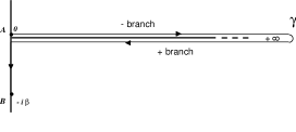
We introduce the Green function
| (5) |
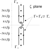
which is path-ordered on the oriented contour of Fig. 1. In Eq. (5) is the complex variable running on with , while and are the end-points of . Further, and are Heisenberg operators defined by the non-unitary evolution operator for complex times . They are in general not Hermitian conjugates of one another, but the usual equal-time anticommutation relations are still obeyed.
As before the average is the grand-canonical average. On the vertical track going from 0 to we have independent of . Therefore, the Green function satisfies the relations
| (6) |
Next, we write the total Hamiltonian as the sum of a diagonal term and an off-diagonal one
The quantities and are constants on the vertical track. [The decomposition above is completely general. In our model examples discussed later, the diagonal part will represent an uncontacted system and the off-diagonal the contacts.] The Green function is obtained by solving the equation of motion
| (7) |
[and its adjoint] with boundary conditions (6). We define as the uncontacted Green function. The satisfies Eq. (7) with and obeys the same boundary conditions of the contacted . The unique resulting from such a scheme belongs to the Keldysh spacedaniele and can be written as
where if is later than on and zero otherwise. is analytic for any later than while is analytic for any later than ; they are given by
| (8) |
where and the integral appearing in the exponential function is a contour integral along going from to . Choosing and on the real axis and reduce to the real-time lesser and greater component. From Eqs. (8) one can easily verify that the corresponding retarded and advanced component can be written as
| (9) |
The uncontacted allows to convert Eqs. (7) into an integral equation which preserves the relations (6):
| (10) |
Using the Langreth theoremlangreth one finds
| (11) |
where we have used the short hand notation to denote integrals along the real axis, going from 0 to , and for integrals along the imaginary vertical track, going from 0 to . For the sake of clarity we have also introduced the symbols and : any function with the superscript is intended to have a real first argument and an imaginary second argument; the opposite is specified by . In Eq. (11), ; for we don’t need to say more since it is always foregone and followed by or so that no ambiguity arises. In particular we note that implies a simple matrix multiplication since along the vertical track is a constant matrix times the delta function.
The equation for contains with one real and one imaginary argument. This coupling does not allow to get a closed equation for with two real arguments, unless on the vertical track. Conversely, and satisfy an integral equation without any coupling:
| (12) |
Eq. (11) can be solved for and one obtains
| (13) | |||||
From Eq. (8) and Eq. (9) we have and , so that Eq. (13) can be rewritten as
| (14) | |||||
The above expression for deserves a brief comment. Indeed, the first term on the r.h.s. is exactly what one got in the partitioned approach, where the hopping parameters vanish along the vertical track. It is usually argued that if the second term vanishes. However, we point out that in the noninteracting case this is not true. If in the long-time limit some physical response functions, e.g., the current, are correctly reproduced by using the partitioned other kind of argumentations should be invoked. We shall come to this point later on.
II.2 Interacting Systems in the Presence of an External Disturbance
In the interacting case we keep track of the interactions by introducing a self-energy matrix. Then, Eq. (7) becomes
| (18) |
Here is the self-energy part which is local in time and it consists of a Hartree and an exchange term. The remaining part of the self energy contains the contributions coming from the correlation and belongs to the Keldysh space:daniele
Like , the self energy and its components are matrices in the one-electron labels. No simple expressions, like (3)-(4), can now be directly obtained from the equation of motion and the Keldysh formalism is unavoidable.
A proper treatment of the initial correlations naturally leads to an extension of the Keldysh equations. The generalization was put forth by Wagnerwagner who obtained a minimal set of five independent integro-differential equations for the unknowns , , (or ) (or the Keldysh Green function ), (or ) and the thermal Green function with two imaginary arguments. In Appendix A we exploit the results of the previous Subsection to prove that the solution for can be written as
| (19) |
where
This result clearly reduces to Eq. (17) if the self energy vanishes since . We observe that if the Green functions vanish when the separation of their time arguments goes to infinity, Eq. (19) yields a well known identity
| (20) |
Eq. (20) is well suited to study the long-time response of an interacting system subjected to an external time-dependent disturbance. On the other hand, if one is interested in the short-time response Eq. (19) cannot be simplified. In some cases it might be simpler to use an alternative approach. Below we propose an exact non-equilibrium Green function treatment based on TDDFT and discuss the relations to ordinary Mean Field approximations.
II.3 Mean Field Theory and Relations to TDDFT
Any Mean Field Theory is a one-particle-like approximation in which each particle moves in an effective average potential independently of all other particles. The mean-field potential is local in time, meaning that is discarded. Consequently, all the results of the Section II.1 can be reused provided we substitute by . Thus, no extra complications arise if we treat an interacting system at the Hartree-Fock level. To be specific, let us focus on the Coulomb interaction and on paramagnetic systems (so that the self energy and the Green function are diagonal in the spin indices). Then, it is natural to choose the one-electron index as the coordinate of the particle and to split the self energy as a sum of the Hartree and the exchange term
For extended systems, the Hartree potential and the Coulomb potential from the nuclei are separately infinite but with a finite sum. Together with the external field these terms form the classical electrostatic potential . The Green function can be obtained from the self-consistent solution of the equation of motion and the lesser/greater component can be written as
where the subscript MF has been used to stress that it is a Mean Field approximate result. In the ordinary Many Body Theory one has to abandon the one-particle picture in order to improve the approximation beyond the Hartree-Fock level. This leads to a self energy nonlocal in time and hence to the complicated solution (19).
In the case we only ask for the density the original Density Functional Theoryhk ; ks and its finite-temperature generalizationmermin has been extended to time-dependent phenomena.rg ; litong The theory applies only to those cases where the external disturbance is local in space, i.e., . For we switch on an external potential to obtain a density . The Runge-Gross theorem states that if we instead had switched on a different [giving a different ], then implies . Thus is a unique functional of . Runge and Gross also show that one can compute in a one-particle manner using an effective potential
Here, accounts for exchange and correlations and is obtained from an exchange-correlation action functional, . In our earlier language this corresponds to an effective self energy which is local in both space and time. The TDDFT one-particle scheme corresponds to a fictitious Green function which satisfies the equations of motion (7) with replaced by . As a consequence we have
The fictitious will not in general give correct one-particle properties. However by definition gives the correct density
(where the factor of 2 comes from spin). Also total currents are correctly given by TDDFT. If for instance is the total current from a particular region we have
| (21) |
where the space integral extends over the region ( is the electron charge).
The Density Functional Theory and the Runge-Gross extension refer specifically to the basis. However, the arguments remain valid if we instead consider the diagonal density in some other basis provided the interactions commute with the diagonal density operator. The latter condition is essential for the Runge-Gross theorem. Thus, for instance, if the one-electron indices refer to a particular lead one can still use Eq. (21) to calculate the corresponding total current (see Section IV).
For later references we now derive an expression for the lesser/greater Green function in the linear approximation. We consider the partition-free system described in the one-particle scheme of Mean Field Theory or TDDFT. Let be the small time-dependent effective perturbation and be the first order variation of the retarded and advanced Green functions with respect to their equilibrium counterparts . Then, from Eq. (17) we get
| (22) | |||
where we have taken into account that commutes with . The above expression takes an elegant form when . Indeed, for any one has and . Since the integrands in Eq. (22) vanish for due to the function in in the first term and in in the second term, we conclude that for any positive time
| (23) |
We shall use this equation later on to calculate the linear current response in noninteracting and interacting resonant tunneling systems.
III Noninteracting Resonant Tunneling Systems
As a first application of the partition-free approach we study the time-dependent current response of a noninteracting resonant tunneling system. For the sake of simplicity the central device will be modeled by a single localized level. All the results of this Section can be generalized to the case of a multi-level noninteracting central device without any conceptual complications. There are many different geometries one can conceive beyond a one-level model, e.g., a double quantum dots model,ziegler a quantum wire coupled to a quantum dot,liang a one-dimensional quantum-dot arrayshangguam or a mesoscopic multi-terminal system.sun However, the present paper is not intended to give a description of a series of applications. Rather, we prefer to illustrate how the partition-free approach works in a simple noninteracting model. We also emphasize that all the results of this Section remain valid in the interacting case if the bare external potential is replaced by the exact effective potential of TDDFT, see Section IV.
The whole system is described by a quadratic Hamiltonian
where denotes the left, right lead and are collective indices for and 0. We assume the system in thermodynamic equilibrium at a given inverse temperature and chemical potential before the time-dependent perturbation
is switched on. In principle the time-dependent perturbation may have off-diagonal matrix elements. In order to model a uniform potential deep inside the electrodes such off-diagonal terms must be of lower order with respect to the system size. However their inclusion is trivial and it does not lead to any qualitative changes.
The current from the contact through the barrier to the central region can be calculated from the time evolution of the occupation number operator of the contact. From the obvious generalization of Eq. (21) one readily finds
The above expression is manifestly gauge-invariant. Indeed, if then while and the time-dependent shift has no effect on the current response. In the same way it is invariant under a simultaneous shift of and the initial potential.
The matrix can be written aslw
where is the contour surrounding all the Matzubara frequencies clockwise [see Fig. 9 in Appendix C] while is an infinitesimally small positive constant. It is therefore convenient to define the kernel
| (26) |
with , and to write the current in the form
| (27) |
It is worth noticing that the partitioned approach leads to Eq. (III) with in place of . It is our intention to clarify under what circumstances, if any, the long-time behavior of the time-dependent current is not affected by this replacement.
As a side remark we also observe that in Eq. (III) correctly vanishes. Letting and be the eigenvectors and eigenvalues of , we have
since and can always be chosen as real quantities for systems with time reversal symmetry.
III.1 Step-Like Modulation
The first exactly solvable model we wish to consider is a step-like modulation, i.e., . From Eq. (3) it follows that for any
and . The device component of can be written as
| (28) |
where . Here, is the retarded/advanced self energy induced by back and forth virtual hopping processes from the localized level to the leads and is given by
| (29) |
where we have used the short-hand notation .
III.1.1 : Steady-State Current
If the energy levels of the lead are equally shifted. From Eq. (III) it follows that we need to estimate the matrix elements , of the retarded Green function and the two contractions , in the long-time limit. We assume that is a smooth function for all real . Then, using the the Riemann-Lebesgue theorem one can prove (see Appendix B) that the kernel has the following asymptotic behavior
| (30) | |||
where
| (31) |
In Eq. (30) the r.h.s. has a simple pole structure in the variable and therefore the integration along the contour can be easily performed. Using the identity the stationary current has the following expression
| (32) | |||||
where is the Hilbert transform of :
| (33) |
It is of interest to note that the dependence on the bias appears not only in the distribution function but also in the quantities and , see Eqs. (31)-(33). The dependence of the self energy on the level-shifts is physical since when the particle visits the reservoirs experiences the applied potential. We also remark that Eq. (32) is of the Landauer type.landauer More generally the Landauer formula is valid for any mesoscopic device provided it is noninteracting. This result agrees with the one obtained in the partitioned approach by Jauho and coworkers.jauho ; haug There the leads are decoupled from the central device and in thermal equilibrium at different chemical potential and and inverse temperature and in the remote past. In order to preserve charge neutrality each energy level must be shifted by where is the chemical potential of the two undisturbed leads. The stationary current is then obtained by switching on the contacts, i.e., the hybridization part of the Hamiltonian. By tuning and the current is given by Eq. (32).
To summarize we have found that for noninteracting leads a steady state develops in the long-time limit whenever 1) The one-body levels of the charge reservoirs form a continuum and 2) The self energy due to the hopping term is a smooth function. Under these hypotheses the time-translational invariance is restored by means of a dephasing mechanism. The comparison of our result with the one obtained in the partitioned scheme provides the criteria of equivalence: besides the tuning one needs to shift the levels of the reservoir by .
III.1.2 : Time-Dependent Current in the Wide-Band Limit
The calculation of the stationary current is greatly simplified by the long-time behavior of the various terms coming from Eq. (III). However, as far as we are interested in the current at any finite time we need to specify the structure of the retarded (advanced) self energy. Here, we consider the so called wide-band limit where the level-width functions are assumed to be constant and hence, from Eq. (33), . In this case has a simple-pole structure and the calculations are slightly simplified. We emphasize that what follows is the first explicit result of a time-dependent current in a model system in the framework of a partition-free approach and therefore also a simple model could be of some interest. Without loss of generality we can always choose ; for the sake of simplicity we also consider . We defer the reader to Appendix C for the details. Here, we just write down the final result for :
| (34) | |||
where is the stationary current of Eq. (32) and . One can easily check that 1) For Eq. (34) yields the result in Eq. (32), 2) For the current vanishes, that is and 3) For the current vanishes for any . Eq. (34) can be rewritten in a more physical and compact way if we exploit the particle-number conservation. Denoting by the particle number operator in the central device we have
so that
is obtained by exchanging in the r.h.s. of the above expression. Therefore, for any finite time , even in the symmetric case ; the time derivative of contributes to and in the same way.
Our formula for the nonlinear transient current clearly differ from the one obtained by Jauho et al.jauho in the partitioned scheme. Indeed, the prescribed integration along the imaginary axis gives extra terms (see Appendix C) which are absent if the system is uncontacted for negative times. We have explicitly verified that by discarding these terms our formula reduces to the one obtained in the partitioned scheme. For long times, the extra terms vanish and our scheme reproduces the earlier steady-state results.
If one of the two leads does not undergo any level shift, e.g. , from Eq. (34) we get
| (35) | |||
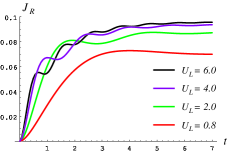
The transient behavior of the time-dependent quantity is not simply an exponential decay. In Fig. 2 we have plotted in Eq. (35) versus for different values of the applied bias at zero temperature. The current strongly depends on for small while it is fairly independent of it in the strong bias regime; using the parameter specified in the caption, the time-dependent current has essentially the same shape for any .
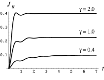
In Fig. 3 the current is plotted for different values of the total line width and for a fixed value of the applied bias. As expected, the larger is the bigger is the slope of the current in .
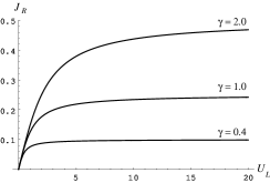
Finally, in Fig. 4 we report the trend of the stationary current as a function of the bias for three different choices of the level widths. As one can see the bigger is and the wider is the range of validity of the Ohm law.
III.2 Arbitrary Modulation: Theorem of Equivalence
We have shown that the steady-state current induced by a step-like modulation does not change if one uses the of the partitioned approach, given by the first term on the r.h.s. of Eq. (14), in place of the one coming from the partition-free approach. This reasonable result is now proved and not simply postulated. The equivalence between the two expressions for the current is of special importance since it is much easier to work in the partitioned scheme. However, it has been proved only for step-like modulations with . Here, we prove that the above equivalence remains true under very general assumptions. To this end we consider the quantity
| (36) |
where is an arbitrary complex function of . Then, the following theorem holds
Theorem of Equivalence: If
| (37) |
for any nonsingular , then
| (38) |
where , and is the uncontacted Green function.
Eq. (38) says that if we apply the same time-dependent perturbation the same asymptotic current will emerge in the partitioned and partition-free approaches.
Proof: In terms of the self energy , the equation of motion for takes the form
where the symbol denotes the real-time convolution. We now consider the limit . The hypothesis (37) implies
| (39) |
which in turn implies that . Furthermore, from the Dyson equation for we find
| (40) |
We note that the above two asymptotic relations have been obtained for in the special case of a step-like modulation, see Eq. (60). Here, we have shown that they hold in a more general context. As a consequence of these two identities, the asymptotic difference can be written as
Here, is given by Eq. (36) with . Since , and hence is nonsingular, meaning that Eq. (37) holds. Eq. (37) together with Eq. (40) imply the equation of equivalence (38).
As a simple application of the Theorem of Equivalence one can calculate the stationary current for an arbitrary step-like modulation. The quantity is simply given by the first two terms of Eq. (61). Both have a simple pole structure in the variable and we can perform the integration along the contour . Using the definition in Eq. (31), with , one obtains
The quantity is the equilibrium line width. Eq. (III.2) reduces to Eq. (32) if since in this case .
In the noninteracting case it is reasonable to assume that Eq. (III.2) yields the steady-state current even for an arbitrary time-dependent disturbance such that and . In the next Section we shall prove that the asymptotic current has no memory and depends only on the asymptotic value of the external perturbation.
III.3 Memory Loss Theorem
If the condition (37) of the Theorem of Equivalence is fulfilled, the asymptotic value of the nonlinear time-dependent current in Eq. (27) simplifies to
We note in passing that expressing and in terms of and respectively, Eq. (III.3) can be rewritten in terms of
where the asymptotic relation has been used [see Eq. (20)]. This agrees with the result obtained by Wingreen et al.wingreen ; jauho in the partitioned approach, as it should.
In general is not a constant unless the external perturbation tends to a constant in the distant future. In this case the following theorem holds
Memory Loss Theorem: If
the current tends to a constant, given by Eq. (III.2), in the long-time limit.
Proof: Is convenient to denote with and the Green functions corresponding to the step-like modulation with coefficients and . We have already shown that in the long-time limit Eq. (III.3) yields Eq. (III.2) if . The Memory Loss Theorem is then proved if
| (43) |
for some real constant .
According to Eq. (39), the device component of the retarded Green function vanishes for any finite . Since , from it follows that . Let us now consider the Dyson equation
| (44) |
with and . Since the integrand vanishes for any finite , we can substitute with . Furthermore, since the applied bias tends to a constant in the distant future, for some real quantity . The l.h.s. of Eq. (43) is then proved. A similar reasoning leads to the r.h.s. of Eq. (43).
III.4 Linear Response in the Wide-Band Limit
In the case of small time-dependent perturbations, one can use Eq. (23) to calculate the lesser Green function. In order to carry on the calculations analytically we consider the wide-band limit and we choose . For simplicity we omit the subscript 0 in the retarded and advanced equilibrium Green functions. By explicitly writing down the matrix product in Eq. (23) one readily realize that we have to calculate the functions , , and . They are easily obtained from Eqs. (63) by simply replacing and . The calculations are rather similar to those already performed to derive the expression (34) and they are left to the reader. Denoting by the time-dependent current in the linear regime one ends up with
| (45) |
where . In the special case , and const, reduces to the time-dependent current in Eq. (34) to first order in , as it should.
Eq. (45) takes a very simple form if and :
where are the Matzubara frequencies and the identity
has been used. In the special case of a vanishing chemical potential, the Matzubara frequencies are imaginary numbers and simplifies
| (46) |
where
is a linear combination of the Lerch transcendent functions .
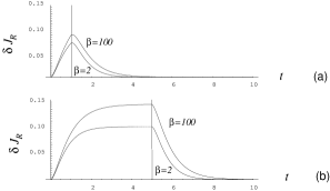
In Fig. 5 we show the trend of for square bump-like modulations. On the top while on the bottom ; both disturbances are considered for two different inverse temperature and . As one can see the effect of an increasing temperature consists in a sort of rescaling of the time-dependent current. The line widths have been taken equal and large enough to justify the linear approximation. Since the disturbance is of order 1, from Fig. 4 one can see that is a good choice.
IV Interacting Systems
In earlier theoretical works on quantum transport one can distinguish at least two schools. In one school one tries to keep the full atomistic structure of the conductor and the leads, but all works so far are at the level of the Local Density Approximation (LDA) and only the steady state has been considered. The advantage of this approach is that the interaction in the leads and in the conductor are treated on the same footing via self-consistent calculations on the current-carrying system. It also allows for detailed studies of how the contacts influence the conductance properties.
The other school is using simplified models which allows the analysis to be carried much further. Considerable progresses have been made in this respect for a localized level described by a Lundquist-like modelkral ; lundin ; xin and for the so called “Coulomb island”meir ; you where in Eq. (III) is replaced by the Anderson Hamiltonian. However, all these works treat the leads as non-interacting, which prohibits a realistic description of the contacts and of the long-range aspects of the Coulomb interactionB ttiker . The model approach are based on a partitioned scheme which makes the time-dependent results difficult to interpret.
We here want to show how the current LDA by Lang et al.Lang1 ; Lang2 follows from the TDDFT scheme described in Section II.3. We also present an exact result for the steady-state current of an interacting resonant tunneling system. Finally, the transient behavior of a capacitor-device-capacitor system is investigated on the level of Mean Field.
IV.1 Steady-State Limit of TDDFT
In Section III we showed that under certain conditions a steady state is reached in the long-time limit, and that this limit is independent of history. We also showed that the partitioned and partition-free treatments give an equivalent description of the steady state. The mechanism for the loss of memory was pure dephasing, and it holds provided the leads are macroscopic while the device is finite. Another important ingredient is that the applied bias is uniform deep inside the leads. With these assumptions, our results can be generalized also to more general cases than the simplified model explicitly considered in Section III. In TDDFT, the full interacting problem is reduced to a fictitious noninteracting one and all the results of Section III can be recycled. In the case of Time Dependent Local Density Approximation (TDLDA), the exchange-correlation potential depends only on the instantaneous local density and has no memory at all. If the density tends to a constant, so does the effective potential , which again implies that the density tends to a constant. Owing to the non-linearity of the problem there might still be more than one steady-state solution or none at all.
If a steady state is reached in TDDFT, we can go directly to the long-time limit of the Dyson equation and work in the frequency space. We may with no restriction use a partitioned approach and split the fictitious one-electron Hamiltonian matrix in a non-conducting part and a correction involving one-body hopping terms between the two leads and the device. The lesser Green function of TDDFT fulfills
where is the uncontacted TDDFT Green function [cf. Eq. (13)]. In direct space, the uncontacted can be written
in terms of diagonalizing orbitals with fictitious eigenvalues for the left and right leads () and the device () and Fermi functions with chemical potential . The chemical potentials for the two leads differ, and the final result is independent of the chosen chemical potential for the device. When we apply to an unperturbed orbital , it is transformed to an interacting, i.e., contacted eigenstate . Above the conductance threshold, states originating from the left lead become right-going scattering states, and states from the right lead become left-going scattering states. In addition, fully reflected waves and discrete state may arise which contribute to the density but not to the current. Thus,
These results correspond closely to the general approach by Lang and coworkers.Lang1 ; Lang2 In their approach, the continuum is split into left and right-going parts, which are populated according to two different chemical potentials. The density is then calculated self-consistently. Lang et al. further approximate exchange and correlation by the LDA and the leads by homogeneous jellia, but apart from these approximations it is clear that his method implements TDDFT, as described in Section II.3, in the steady state. It is also clear that the correctness of Lang’s approach relies on the Theorem of Equivalence between the partitioned and partition-free approaches and the Memory Loss Theorem derived here. The equivalence between the scattering state approach by Lang et al. and the partitioned non-equilibrium approach used by Taylor et al.Taylor1 ; Taylor2 has also been shown by Brandbyge et al.brand
As shown above, the steady state of TDDFT can always be formulated in terms of orbitals which diagonalize the asymptotic one-particle Hamiltonian matrix. The current-carrying orbitals can always be grouped into a right-going class and a left-going class. As a consequence, the current can be expressed in a Landauer formula
| (47) |
in terms of fictitious transmission coefficients and energy eigenvalues , . We also wish to emphasize that the steady-state current in Eq. (47) comes out from a pure dephasing mechanism in the fictitious noninteracting problem. The memory-loss effects from scatterings is described by and .
IV.2 One-Level Resonant Tunneling System
In this Section we consider a resonant tunneling system described by the quadratic Hamiltonian of Eq. (III) and an inter-particle interaction
where is the occupation number operator of the level and is a symmetric matrix. (If includes long-range terms, the regrouping of potential terms as discussed in Section II.3 must be done.) In the generalized TDDFT scheme (based on the occupations rather than on density) outlined in Section II.3 the fictitious Green function is obtained by solving the Dyson equations with , where
If satisfies the hypothesis of the Theorem of Equivalence and of the Memory Loss Theorem we can use Eq. (III.2) and write an exact formula for the steady-state current of an interacting resonant tunneling system:
For normal-metal electrodes we expect that the effective potential provided when . The constant may depend on the history of while the steady-state current is independent of the history of . is given by Eq.(28) with and with from Eq.(29) with . For the sake of clarity, Eq. (IV.2) has been written for systems having a one-to-one correspondence between the one-body indices and the one-body energies . The generalization to systems with degenerate levels is straightforward and it is left to the reader.
As a further example we study the RPA time-dependent current response in the partition-free approach. In the Hartree approximation the Green function satisfies the equation of motion (18) with and
where . According with the results obtained in Section II, the lesser Green function is given by Eq. (17) with . Therefore, in the linear approximation we have
| (49) | |||
with
| (50) |
Eqs. (49)-(50) form a coupled system of integral equations for the unknowns and . For a capacitor-device-capacitor system one can take
Thus, putting an extra particle in the isolated capacitor costs an energy per particle. This means that the transfer of a finite number of particles from one capacitor to the other causes a finite change of the effective applied bias. We expect that the current vanishes in the long-time limit unless the applied bias continues to grow up. The coefficients mimic the repulsion energy between two particles in different capacitors. Actually, one can also consider the interaction between a particle in the central device and another in one of the two capacitors. No extra complications arise if , , and the results we are going to obtain can be easily extended.
Switching a bias , from Eq. (50) one gets with , , and
| (51) |
where it has been taken into account that . Since has the same matrix structure of the bare , in the wide-band limit the linear time-dependent current is given by Eq. (45) with replaced by . (It is worth noticing that the wide band limit still makes sense if the line width is approximately constant in a small interval around the chemical potential .) In this way the system of Eqs. (49)-(50) is reduced to a system of 4 coupled integral equations for the 4 scalar unknowns , with . The symmetric case , allows a further simplification. Let us define , , and . Then, from Eq. (51) we find
| (52) |
while from Eq. (45)
| (53) |
| (54) |
where
is the conductivity kernel. Once has been obtained, one can calculate and .
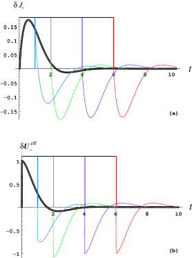
In order to illustrate what is the time-dependent response of this model we have considered the zero temperature case with and . Then, and hence . It follows that and for any time . In Fig. 8(a) we display the time-dependent current for square bump-like modulations with and . The thick line is the current for the step like modulation ; depending on the value of the current unsticks itself from the thick line giving rise to different damped oscillating curves. In correspondence of each a vertical line has been drawn; it represents the bare applied potential . Fig. 8(b) shows the time-dependent effective potential . As the current response, it drops to zero in the long-time limit since the interactions completely screen the applied bias after a time .
V Summary and Concluding Remarks
In the present work we have used a partition-free scheme in order to treat the time-dependent current response of a mesoscopic system coupled to macroscopic leads. To this end, we have further developed the Keldysh formalism and we have formulated a formally exact theory which is more akin to the way the experiments are carried out. Among the advantages of the partition-free scheme we stress the possibility to calculate physical dynamical responses and to include the interactions between the leads and between the leads and the device in a quite natural way.
In the noninteracting case we have shown that a perfect destructive interference takes place provided the energy levels of the leads form a continuum. The steady-state develops due to a dephasing mechanism. The comparison of our steady-state current with that obtained in the partitioned scheme shows that the two currents are equivalent if the energy levels are properly shifted in order to preserve charge neutrality. This kind of equivalence remains true for any time-dependent external potentials (Theorem of Equivalence). The Theorem of Equivalence has then been used in order to prove that the steady-state current depends only on the asymptotic value of the external perturbation (Memory Loss Theorem). For the sake of clarity, the Theorem of Equivalence and the Memory Loss Theorem have been proved for a single-level central device. The generalization to a multi-level central device is straightforward, as can be readily verified. In the wide band limit we have obtained an analytic result for the time-dependent current in the case of a step-like modulation and for arbitrary modulations in the linear regime.
The interacting case represents a more difficult challenge and the expression for the lesser Green function at any finite time is more complicated than that commonly used to calculate steady-state response functions. As an alternative to a full many-body treatment we have proposed a formally exact one-particle scheme based on TDDFT. Then, all the results obtained in the noninteracting case can be recycled provided we substitute the external potential with the exact effective potential of TDDFT. Although it is difficult to prove any rigorous results for the effective TDDFT potential, we expect the interactions to reduce the memory effects even further compared to the noninteracting case. Thus, any nonlinear steady-state current can been expressed in a Landauer-like formula in terms of fictitious transmission coefficients and one-particle energy eigenvalues. The steady-state current depends on history only through the asymptotic shape of the effective TDDFT potential. This exact result may prompt for new approximations to the exchange-correlation action functional . In the effective one-particle scheme of TDDFT the steady-state current comes out from a pure dephasing mechanism. The damping mechanism (due to the electron-electron scatterings) of the real problem is described by . As an illustrative example we have also calculated the RPA time-dependent current of a capacitor-device-capacitor system and we have displayed the effect of the charge oscillations in the discharge process.
Acknowledgements.
We would like to acknowledge useful discussions with U. von Barth, P. Bokes, M. Cini, R. Godby, A.-P. Jahuo, B. I. Lundqvist, P. Hyldgaard, and B. Tobiyaszewska. This work was supported by the RTN program of the European Union NANOPHASE (contract HPRN-CT-2000-00167).Appendix A Proof of Eq. (19)
It is convenient to define as the solution of Eqs. (18) with . satisfies all the relations we have derived for a noninteracting system in the presence of an external disturbance. By using the Langreth theorem, we get
and solving for
Next, we use
and
so that
| (55) | |||
As in the noninteracting case, we proceed by writing down the Dyson equation for . Taking into account that
| (56) |
and that
we have
| (57) |
Similarly, it is straightforward to show that
| (58) |
Substituting Eq. (57) into Eq. (55) and using Eq. (56) one finds
| (59) | |||||
Using Eqs. (57)-(58) to express the last two terms as
and
we end up with Eq. (19).
Appendix B Proof of Eq. (30)
Due to the smoothness of the self energy, in the long-time limit we can use the Riemann-Lebesgue theorem to obtain the following asymptotic behaviors
| (60) |
and
From the above results and the definition (26) one has
Appendix C Proof of Eq. (34)
The quantity involves the multiplication of three matrices and we can recognize four contributions, two containing and other two containing . It is straightforward to verify that
| (62) |
and that , where . Hence
| (63) | |||
Eqs. (62)-(63) are all what we need in order to evaluate the quantity in Eq. (26). The time-dependent current is then obtained integrating over along the contour of Fig. 9, according with Eq. (27). Using Eqs. (63) and expressing and in terms of we obtain
| (64) |
| (65) | |||
We are left with the contributions containing . One of them is quite easy to evaluate and yields:
| (66) | |||
The other one is much more involved, but nothing more than standard algebra is needed to get the following expression
| (67) | |||
The r.h.s. of the above four equations must now be multiplied by and integrated over along the contour . Smearing the branches and on the real axis and taking into account Eq. (62), the r.h.s. of Eq. (64) yields the following contribution to the current
| (68) |
where the integration over has to be understood from to . Another contribution comes from the first term on the r.h.s. of Eq. (65). By closing the contour of the integration on the complex upper half plane, it is non vanishing only if . Therefore, only the upper branch of contributes. can then be smeared on the real axis and one gets
| (69) |
A similar procedure can be adopted to evaluate the contribution coming from the second term on the r.h.s. of Eq. (65). One more time we can close the contour of the integration on the complex upper half plane. The pole in does not contribute since its residue is zero. The other pole is in and hence one obtains
| (70) |
Next, we have to calculate the contribution coming from Eq. (66). By the same reasoning leading to Eq. (70) it is readily verified that it yields the same result. Therefore we have to keep in mind that Eq. (70) should be multiplied by 2 at the end. Let us now consider the contribution coming from the first two terms on the r.h.s. of Eq. (67). Since the discontinuous function does not appear in the integrand we can perform the contour integral over . We find
The contribution coming from the last two terms on the r.h.s. of Eq. (67) vanishes. Indeed the integral over can be closed on the complex lower half plane. The pole in does not contribute since its residue is zero. The other pole contributes only if . At the same time we can also perform the integration over by closing the contour in the complex upper half plane. The first term in the square brackets of Eq. (67) is non vanishing only if . The same holds for the second term since the pole has vanishing residue. By collecting all the results obtained one sees that they can be grouped into three broad categories: those which are time independent and that give rise to the stationary current, those which are proportional to and those which are proportional to . These last ones can be rewritten as
| (72) |
Let us now group the terms proportional to . Two of them comes from Eq. (69) and the first term of Eq. (C); their sum can be written as
| (73) |
The other two pieces come from Eq. (70) (which we recall must be multiplied by 2) and the last term of Eq. (C). By writing explicitly the real part, after some algebra one finds
| (74) | |||
The sum of Eqs. (72)-(73)-(74) gives exactly the quantity of Eq. (34).
References
- (1) C. Caroli, R. Combescot, P. Nozìeres, and D. Saint-James, J. Phys. C 4, 916 (1971).
- (2) C. Caroli, R. Combescot, D. Lederer, P. Nozìeres, and D. Saint-James, J. Phys. C 4, 2598 (1971).
- (3) T. E. Feuchtwang, Phys. Rev. B 10, 4121 (1974).
- (4) T. E. Feuchtwang, Phys. Rev. B 10, 4135 (1974).
- (5) L. P. Kadanoff and G. Baym, Quantum Statistical Mechanics (W. A. Benjamin, Inc. New York, 1962).
- (6) L. V. Keldysh, JETP 20, 1018 (1965).
- (7) Ned S. Wingreen, A.-P. Jauho, and Y. Meir, Phys. Rev. B 48, 8487 (1993).
- (8) A.-P. Jauho, N. S. Wingreen, and Y. Meir, Phys. Rev. B 50, 5528 (1994).
- (9) A.-P. Jauho, cond-mat/9911282 (unpublished).
- (10) H. Haug and A.-P. Jauho, Quantum Kinetics in Transport and Optics of Semiconductor (Springer-Verlag, Berlin, 1998).
- (11) M. Cini, Phys. Rev. B 22, 5887 (1980).
- (12) E. Runge and E. K. U. Gross, Phys. Rev. Lett. 52, 997 (1984); for on the Keldysh contour see also R. van Leeuwen, Phys. Rev. Lett. 80, 1280 (1998).
- (13) N. D. Lang, Phys. Rev. B 52, 5335 (1995).
- (14) N. D. Lang and P. Avouris, Phys. Rev. Lett. 81, 3515 (1998).
- (15) J. Taylor, H. Guo, and J. Wang, Phys. Rev. B 63, 121104 (2001).
- (16) J. Taylor, H. Guo, and J. Wang, Phys. Rev. B 63, 245407 (2001).
- (17) A. Blandin, A. Nourtier, and D. W. Hone, J. Phys. (Paris) 37, 369 (1976).
- (18) P. Danielewicz, Ann. Physics 152, 239 (1984).
- (19) D. C. Langreth, in Linear and Nonlinear Electron Transport in Solids, edited by J. T. Devreese and E. van Doren (Plenum, New York, 1976), pp. 3–32.
- (20) M. Wagner, Phys. Rev. B 44, 6104 (1991).
- (21) P. Hohenberg and W. Kohn, Phys. Rev. 136, B 864 (1964).
- (22) W. Kohn and L. J. Sham, Phys. Rev. 140, A 1133 (1965).
- (23) N. D. Mermin, Phys. Rev. 137, A 1441 (1965).
- (24) Tie-cheng Li and Pei-qing Tong, Phys. Rev. A 31, 1950 (1985).
- (25) R. Ziegler, C. Bruder, and H. Schoeller, Phys. Rev. B 62, 1961 (2000).
- (26) Y.-L. Liu and T. K. Ng, Phys. Rev. B 61, 2911 (2000).
- (27) W. Z. Shangguan, T. C. A. Yeung, Y. B. Yu, and C. H. Kam, Phys. Rev. B 63, 235323 (2001).
- (28) Q. feng Sun, B. geng Wang, J. Wang, and T. han Lin, Phys. Rev. B 61, 4754 (2000).
- (29) J. M. Luttinger and J. C. Ward, Phys. Rev. 118, 1417 (1960).
- (30) R. Landauer, IBM J. Res. Dev. 1, 233 (1957).
- (31) P. Kral and A. P. Jauho, Phys. Rev. B 59, 7656 (1999).
- (32) U. Lundin and R. H. McKenzie, Phys. Rev. B 66, 075303 (2002).
- (33) J.-X. Zhu and A. V. Balatsky, Phys. Rev. B 67, 165326 (2003).
- (34) Y. Meir and N. S. Wingreen, Phys. Rev. Lett. 68, 2512 (1992).
- (35) J. Q. You, C.-H. Lam, and H. Z. Zheng, Phys. Rev. B 62, 1978 (2000).
- (36) M. Büttiker, J. Phys.: Condens. Matter 5, 9361 (1993).
- (37) M. Brandbyge et al., Phys. Rev. B 65, 165401 (2002).