Aging in Spin Glasses in three, four and infinite dimensions

Abstract

The SUE machine is used to extend by a factor of 1000 the time-scale of previous studies of the aging, out-of-equilibrium dynamics of the Edwards-Anderson model with binary couplings, on large lattices ($L=60$). The correlation function, $C(t+t_{w},t_{w})$, $t_{w}$ being the time elapsed under a quench from high-temperature, follows nicely a slightly-modified power law for $t>t_{w}$. Very tiny (logarithmic), yet clearly detectable deviations from the full-aging $t/t_{w}$ scaling can be observed. Furthermore, the $t<t_{w}$ data shows clear indications of the presence of more than one time-sector in the aging dynamics. Similar results are found in four-dimensions, but a rather different behaviour is obtained in the infinite-dimensional $z=6$ Viana-Bray model. Most surprisingly, our results in infinite dimensions seem incompatible with dynamical ultrametricity. A detailed study of the link correlation function is presented, suggesting that its aging-properties are the same as for the spin correlation-function.

1 Introduction

Spin-glasses [1, 2, 3, 4] were discovered to age even on human time-scales some twenty years ago [5]. Aging is nicely demonstrated, for instance, in measures of the thermoremanent magnetization (see e.g. [6]): in the presence of a magnetic field, cool an spin-glass from room temperature to the working temperature, $T$, below its glass-temperature; hold the magnetic field for a while (the time elapsed will be called $t_{w}$ hereafter), then switch-off the field and record the time-decay of the magnetization $M_{t_{w}}(t)$. Not only this decay is very slow but, even for the longest $t_{w}$ tried up to now, $M_{t_{w}}(t)$ strongly depends on $t_{w}$ (the larger $t_{w}$ is, the slower decays $M_{t_{w}}(t)$). It has slowly become clear that the important information coming-out from experiments in spin-glasses regards dynamic out-equilibrium effects, such as this one or the more sophisticated memory and rejuvenation effects [7, 6]. Although there has been a burst of theoretical activity in out-of-equilibrium dynamics [8, 9, 10], it is still not clear how out-equilibrium experiments will help us to choose among the conflicting theoretical views on the nature of spin-glasses: Replica-Symmetry Breaking [3] (RSB), the droplets picture [14], and the intermediate TNT picture [15]. The situation is farther complicated by the fact that detailed theoretical predictions (to be confronted with experiments) can be extracted from models only through Monte Carlo simulations[9]. It is worth recalling that numerical results on out-of-equilibrium dynamics have cast some doubts even on the usefulness of the Edwards-Anderson model to describe physical spin-glasses [16] (see however [17] for some reassuring results).

It is thus clear that one needs to address quantitatively the time-decay of $M_{t_{w}}(t)$ or equivalently, given the Fluctuation-Dissipation Theorem [8], the time-dependent correlation function in the absence of a magnetic field:

$$C(t,t_{w})=\frac{1}{N}\sum_{i}\langle\sigma_{i}(t+t_{w})\,\sigma_{i}(t)\rangle$$ (1)

Now, it seems to be a fact of general validity in out-equilibrium dynamics [8] that $C(t,t_{w})$ behaves differently in different time-sectors. Loosing generality for the sake of clarity, this amounts to say that it can be decomposed as

$$C(t,t_{w})=\sum_{i}f_{i}\left(\frac{(t+t_{w})^{1-\mu_{i}}-t_{w}^{1-\mu_{i}}}{1-\mu}\right)\,.$$ (2)

Here, $f_{i}$ are smooth, decreasing functions that tend to zero at infinity, and such that $f_{i}(0)$ is of order one. It follows that if $t\ll t_{w}^{\mu_{i}}$ the $i-th$ time sector contributes the constant value $f_{i}(0)$ to $C(t,t_{w})$, while for $t\gg t_{w}^{\mu_{i}}$ it contributes nothing. In other words, the $i-th$ time sector is active only for $t\sim t_{w}^{\mu_{i}}$ (notice that the different time sectors get neatly separated only in the limit of very large $t_{w}$). Not much is known about the exponents $\mu_{i}$ defining the different time sectors. With this popular parametrization [8, 6], one has $0\leq\mu_{i}\leq 1$. For the simple case of the coarsening-dynamics (domain-growth) of an ordered ferromagnet[18], only two time sectors are needed for a complete description: $\mu_{1}=0$ describing the stationary, $t_{w}$ independent dynamics found at small $t$, and $\mu_{2}=1$ describing the full-aging situation where the correlation-function depends on the ratio $t/t_{w}$. Also the spin-glass dynamics has been experimentally claimed[6] to be ruled only by two time sectors: $\mu_{1}=0$ and $\mu_{2}=0.97$. The second time sector is slightly but clearly different from the full-aging $t/t_{w}$ behavior ($\mu=1$) and is thus named sub-aging. However, a very recent experiment[19] seems to indicate that the sub-aging behavior is just an artifact of the finite-time needed to cool the system down to the working temperature (a limitation not suffered of in numerical simulations). Using their fastest cooling protocol, Rodriguez et al.[19] have found a clear full-aging behavior $\mu_{2}=0.999$. Furthermore, the role of the stationary time-sector ($\mu_{1}=0$) to describe the data is far less critical than previously[6] thought. It is also worth mentioning the recent numerical results in 3 and 4 dimensions by Berthier and Bouchaud [17], who found superaging for infinite cooling rates, turning to subaging for finite cooling rates. At this point, we wish to make two comments:

• The presence of more than two time-sectors seems to be a crucial requirement for the validity of the dynamic version of the usual ultrametric Replica-Symmetry Breaking description of spin-glasses with an infinite number of replica symmetry breakings.

• If the largest $\mu$ exponent is 1, as implied by this popular parametrization [6, 8], for the very large $t_{w}$ achieved in experiments (1 second means roughly $t_{w}=10^{12}$), it is quite possible that all the faster sectors have already died-out since $t_{w}^{\mu_{i}}\ll t_{w}\sim t$. A full-aging ansatz could pretty well describe the data, specially if the second-largest $\mu$ exponent is significantly smaller than one. In this respect, a numerical simulation could have a better chance of observing the different time sectors.

To conclude this introduction, let us recall the main results of previous intensive numerical studies of aging dynamics [9] (for a more recent extensive numerical study of the aging dynamics with a different focus see [16]). Indeed, it was found [9] that the correlation function at short times ($t\ll t_{w}$) could be described as a power law with a temperature dependent exponent ($C(t,t_{w})\sim t^{-x(T)}$). The exponent $x(T)$ was found to be fairly small ($x(T=0.5T_{\mathrm{c}})=0.015$) On the other hand, at long times a power-law decay with a different exponent, $\lambda(T,t_{w})$, was observed ($C(t,t_{w})=t^{-\lambda(T,t_{w})}$ for $t\gg t_{w}$). Yet a cross-over functional form was proposed [20] (see also Ref. [9]), implying that $\lambda(T,t_{w})$ saturates to $\lambda(T)$ for large $t_{w}$:

$$C(t,t_{w})=t^{-x(T)}\Phi\left(\frac{t}{t_{w}}\right)\,.$$ (3)

The cross-over function was proposed to be decreasing, smooth, and to have the asymptotic behaviors $\Phi(y)\sim constant$ for small $y$ and $\Phi(y)\sim y^{-\lambda(T)+x(T)}$ for large $y$. However, in the spanned time scales [9] ($t_{w}\leq 10^{5}$, $t\leq 10^{6}$), $\lambda(T)$ was actually found to significantly depend on $t_{w}$. Yet, if one assumes that $\lambda(T,t_{w})$ saturates to $\lambda(T)$ for large $t_{w}$, so that Eq.(3) could hold, one would speak of a dynamics with effectively three time sectors: $\mu_{1}=0$, $\mu_{2}=1-x(T)/\lambda(T)$, and $\mu_{3}=1$ (to derive this, assume that $\Phi(y)$ is an analytical function, such as $(1+y)^{-\lambda(T)+x(T)}$). However, since $x(T)/\lambda(T)$ was found [9] to be $0.1$ or smaller, it would not be easy to separate the $\mu_{2}$ and $\mu_{3}$ sectors. On the other hand, it is clear that Eq.(3) describes a non-ultrametric dynamics.

In this paper, by extensive Monte Carlo simulations using among others the dedicated SUE machine [21, 22, 23], we will show that there are small yet quite significant deviations to Eq.(3) in finite dimensions. Surprisingly enough, our results in infinite dimensions are rather different, and suggest that dynamical ultrametricity could not hold in (some) statically ultrametric systems. As the reader will notice, heavy use of data fitting will be made in the following. Unfortunately there is no precise theory that tell us which should be the precise functional form of $C(t+t_{w},t_{w})$, so it is difficult to justify theoretically many of the fits. Also the very good power like behaviour we found cannot be recovered from analytic computations. Here we are doing some kind of exploratory work, trying to guess which could be a reasonable form that well represents the data. This may be useful for a number of reasons: If we can do good fits at given vale of $t_{w}$ it is rather more convenient to look to the dependence of the fits parameter on $t_{w}$ than to the data themselves (sometimes scaling plots may be misleading), good fits may evidentiate some behaviour that could be eventually analytically derived, fits can also used to extrapolate data to large times. Finally, notice that as an outcome of this strategy, some of the fits that we are doing could also be useful in analyzing experimental data.

The layout of the rest of this paper is as follows. In section 2 we describe our simulations. In section 3 we concentrate on the spin-spin correlation function, presenting a new parametrization of the function $C(t,t_{w})$, and discussing the possibility of numerically studying the existence of more than two time-sectors. In section 4 we focus on the aging behavior of the link-overlap and the link-correlation function (defined in section 2). We shall conclude that even in the limit of infinite waiting time, the link-correlation function ages. Finally, we present our conclusions in section 5.

2 The simulation

We have studied the three dimensional Ising spin glass defined on a cubic lattice ($L\times L\times L$) with helicoidal boundary conditions. The Hamiltonian is

$${\cal H}=-\sum_{<i,j>}\sigma_{i}J_{ij}\sigma_{j}\ .$$ (4)

The large time scale and lattice sizes simulated have been possible due to the use of a dedicated computer, SUE (Spin Update Engine, Universidad de Zaragoza) based on programmable components, and achieving an update speed of of 0.22 nanoseconds per spin. Details about the machine can be found in Refs. [21, 22, 23].

The volume of the system is $V=L^{3}$, $\sigma_{i}$ are Ising variables, $J_{ij}$ (uncorrelated quenched disorder) are $\pm 1$ with equal probability, and the sum is extended to all pairs of nearest neighbors. The choice of helicoidal boundary conditions is mandatory (for us) because the hardware of the SUE machine has been optimized for them. During the simulation we have measured the following quantities:

$$C(t,t_{w}) = \frac{1}{N}\sum_{i}\ \langle\sigma_{i}(t+t_{w})\,\sigma_{i}(t)\rangle\,,$$ (5)

$$C_{\mathrm{link}}(t,t_{w}) = \frac{1}{DN}\sum_{\mu=1}^{D}\sum_{i}\ \langle\sigma_{i}(t+t_{w})\sigma_{i+\mu}(t+t_{w})\,\sigma_{i}(t_{w})\sigma_{i+\mu}(t_{w})\rangle\,,$$ (6)

$$q(t_{w}) = \left|\frac{1}{N}\sum_{i}\ \langle\sigma_{i}^{(1)}(t_{w})\sigma_{i}^{(2)}(t_{w})\rangle\,\right|\,,$$ (7)

$$q_{\mathrm{link}}(t_{w}) = \frac{1}{DN}\sum_{\mu=1}^{D}\sum_{i}\ \langle\sigma_{i}^{(1)}(t_{w})\sigma_{i+\mu}^{(1)}(t_{w})\,\sigma_{i}^{(2)}(t_{w})\sigma_{i+\mu}^{(2)}(t_{w})\rangle\,.$$ (8)

in the above equations, $D$ is the spatial dimension, $i+\mu$ stands for the nearest neighbor in the $\mu$ direction, while the superscript $(1)$ and $(2)$ refer to the replica index (real replicas: pair of systems evolving independently with the same couplings $J_{i,j}$). The notation $\langle\ldots\rangle$ refers both to average over thermal histories (random-numbers) and over disorder realizations. Let us just recall that since the starting configurations are random, we have explored the so-called $q=0$ sector [3], in which one expects dynamical correlation functions to be self-averaging.

Given the unique features of the SUE machine we have preferred to use it for very long runs in a rather small number of samples. The lattice sizes studied have been $L=20,L=30$ and $L=60$. We have considered three values of the inverse temperature: $\beta=1.25,1.67$ and $2.0$ (hereafter to be referred to as $T=0.8,0.6$ and $T=0.5$ respectively). The critical temperature for this model is $T_{\mathrm{c}}=1.14(1)$, thus the selected temperatures are $0.7T_{\mathrm{c}},0.53T_{\mathrm{c}}$ and $0.44T_{\mathrm{c}}$ respectively. Given the very slow growth of the spin-glass coherence length (see e.g. [9, 24]) one should not expect noticeable finite-size effects even for the $L=20$ lattice. However, as it is well known, sample-to-sample fluctuations in $C(t,t_{w})$ decrease fastly with growing system sizes.

We can sum up the details of the SUE simulations in table 1. The SUE time-step corresponds to 8192 full-lattice sequential heat-bath updates. For $C(t,t_{w})$ and $C_{\mathrm{link}}(t,t_{w})$ we have selected the $t$ and $t_{w}$ values in a logarithmic scale. These values corresponds actually to $8192\times 2^{0.25i},i=1,\dots$. The number of simulated samples has been 16 for the $L=60$ systems and 32 for the $L=20,30$ ones. Here, we will only present the results for $L=60$, since the data for $L=20$ and $L=30$ are fully compatible with them, but far noisier. Yet, much more accurate data have been obtained for moderate $t$ and $t_{w}$ from simulations on a PC (see below) of an $L=33$ system.

L	T	Number of iterations	Number of samples
$60$	$0.5$	$10^{9}$	$16$
$60$	$0.6$	$8\times 10^{8}$	$16$
$60$	$0.8$	$5\times 10^{8}$	$16$
$30$	$0.5$	$5\times 10^{8}$	$32$
$30$	$0.8$	$5.5\times 10^{8}$	$32$
$20$	$0.5$	$2\times 10^{9}$	$32$

Table 1: SUE simulations details

To have some data at times shorter than SUE step $8192$, we have simulated (using heat-bath) on a personal computer 80 samples with $L=60$ ($t_{w}\leq 6877$ , $t\leq 65519$).

In addition, we have performed Metropolis simulations on personal computers for the same model in 3D ($L=33$, $T=0.8=0.7T_{\mathrm{c}}$, $t_{w}\leq 2^{18}$, $t\leq 2^{22}$), 4D ($L=37$, $T=1.2=0.6T_{\mathrm{c}}$, $t_{w}\leq 2^{18}$, $t\leq 2^{22}$ ) and in the infinite-dimensional Viana-Bray model ($z=6$, $N=5\times 10^{6}$, $T=0.8=0.34T_{\mathrm{c}}$, $t_{w}\leq 2^{13}$, $t\leq 2^{17}$ and $N=10^{6}$ $T=0.8$, $t_{w}\leq 2^{19}$, $t\leq 2^{16}$). Even if the times were shorter than in SUE, the number of simulated samples has been much larger. The typical statistical error in correlation functions (as calculated from the sample-to-sample fluctuations) obtained in the PC was 20 times smaller than the statistical errors of the SUE results.

3 Aging dynamics

Figure 1: Double logarithmic plot of the correlation-function obtained with SUE using a heat-bath algorithm, versus $1+t/t_{w}$, for $t_{w}=8192$ and $T=0.5,0.6$ and $0.8$. A single power law fits satisfactorily the data for $t>t_{w}$ at all-three temperatures.

Figure 2: As in Fig.2, for $t_{w}=884736$.

Figure 3: As in Fig.2, for $t_{w}=39813120$.

We have found in finite dimensions ($D=3$ and $D=4$) that the correlation function $C(t,t_{w})$ can be nicely fitted for $t\geq t_{w}$ as

$$C(t,t_{w})=A(t_{w})\left(1+\frac{t}{t_{w}}\right)^{-1/\alpha(t_{w})}\,,\ t>t_{w}.$$ (9)

As it can be seen in Figs. 1,2 and 3, for a wide range of $t/t_{w}$ and $t_{w}$ and all three temperature a simple power-law decay seems enough to describe the data, although the coefficients $A(t_{w})$ and $\alpha(t_{w})$ clearly depends on temperature (notice that $\alpha(t_{w})$ is just the inverse of Rieger et al. [9] $\lambda(T,t_{w})$ exponent). The behavior in infinite dimensions ($z=6$ Viana-Bray model) is rather different and will be discussed at the end of this section.

Figure 4: Top: exponent $\alpha(t_{w})$ defined in Eq.(9) versus $t_{w}$ for the heat-bath dynamics of the Edwards-Anderson model in $D=3$, at $0.7T_{\mathrm{c}}$. Data for $t_{w}<8192$ were obtained on a PC, while for larger $t_{w}$ correlation-functions from SUE were used. Bottom: same as in top panel for the prefactor $A(t_{w})$, defined in Eq.(9). The solid line was obtained fitting for $t_{w}\geq 8192$.

It is clear that the waiting-time dependence of the prefactor $A(t_{w})$ and the exponent $\alpha(t_{w})$ is of utmost importance. Should $A(t_{w})$ and $\alpha(t_{w})$ tend to constant non vanishing values, dynamic ultrametricity [8] would not hold, implying that the usual dynamic formulation of the ultrametric approach to continuous Replica Symmetry Breaking should be modified. Furthermore, we have been unable of finding a divergence law for $\alpha(t_{w})$ compatible with dynamic ultrametricity, if $A(t_{w})$ has a non-vanishing limiting value for large $t_{w}$. Thus, we tend to believe that dynamical ultrametricity implies that $A(t_{w})$ should vanish in the large $t_{w}$ limit.

To obtain the coefficients $A(t_{w})$ and $\alpha(t_{w})$ we have fitted the correlation functions $C(t,t_{w})$ to the functional form in Eq.(9). Yet, although Figs.  1,2 and 3, suggest a pure power-law behavior, we have found some dependence of $\alpha(t_{w})$ on the fitting-window, particularly for $T=0.5$. Specifically, at $T=0.5$ $\alpha(t_{w}=8192)$ grows a $10\%$ if the fit is performed for $t_{w}\leq t\leq 10^{5}t_{w}$ as compared to the fit in the window $t_{w}\leq t\leq 10t_{w}$. Not taking care of this could be dangerous since, obviously, the larger $t_{w}$ the shorter the achievable $t/t_{w}$. Thus, in order to isolate the $t_{w}$-dependence we have restricted ourselves to the fitting range $t_{w}\leq t\leq 10t_{w}$. On the other hand, the prefactor $A(t_{w})$ is basically independent of the fitting-window. Another tricky point is the error-estimate for $A(t_{w})$ and $\alpha(t_{w})$. It is clear that standard techniques ($\chi^{2}$ minimization) work poorly for tremendously correlated stochastic variables such as $C(t,t_{w})$ for successive $t$. In order to have a (hopefully) reasonable estimate we have turned to a Jack-Knife procedure on the fitted coefficients themselves.

Figure 5: As in Fig.4 for $0.53T_{\mathrm{c}}$.

Our results for the prefactor $A(t_{w})$ and the exponent $\alpha(t_{w})$ of the heat-bath dynamics in the $D=3$ case, can be found in Figs. 4 ($T=0.8$), 5 ($T=0.6$) and  6 ($T=0.5$). The results for $t_{w}<8192$ were obtained on a PC (see section 2), while for $t_{w}\geq 8192$ SUE data were used. Actually, we have found that the functional form (9) is not suitable for very small $t_{w}$, thus there is a lower, temperature-dependent, cut-off on the $t_{w}$ values shown in Figs. 4, 5 and 6.

Figure 6: As in Fig.4 for $0.44T_{\mathrm{c}}$.

As far as the exponent $\alpha(t_{w})$ is concerned (see the upper part of Figs. 4, 5 and 6), we have a significant growth for $t_{w}<10^{6}$. For larger $t_{w}$, $\alpha(t_{w})$ is constant within errors. This (asymptotic?) value would correspond to the inverse of the large waiting time limit of Rieger et al. [9] aging exponent $\lambda(T,t_{w})$. Interestingly enough, the values of $\alpha(t_{w})$ for the largest achieved $t_{w}$ seems to be proportional to $T_{\mathrm{c}}/T$. On the other hand, the prefactor $A(t_{w})$ (see the lower part of Figs. 4, 5 and 6) clearly decreases in all the simulated $t_{w}$ range. A power law seems to be appropriate for this decay, the exponent being precisely the exponent $x(T)$ in Eq.(3). Thus, we find $x(0.7\,T_{\mathrm{c}})=0.016$, $x(0.53\,T_{\mathrm{c}})=0.0064$, $x(0.44\,T_{\mathrm{c}})=0.0049$.

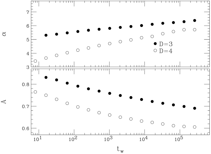
Figure 7: Top: exponent $\alpha(t_{w})$ defined in Eq.(9) versus $t_{w}$ for the Metropolis dynamics of the Edwards-Anderson model in $D=3$ at $T=0.8$ (full circles) and $D=4$ at $T=1.2$ (empty circles). Bottom: same as in top panel for the prefactor $A(t_{w})$, defined in Eq.(9).

We have found similar results (see Fig. 9) for the Metropolis dynamics of the Edwards-Anderson model with binary-couplings distributions in three dimensions ($T=0.7T_{\mathrm{c}}$), four-dimensions ($T=0.6T_{\mathrm{c}}$). For all the simulated $t_{w}$ ($<10^{6}$) we have found a growing trend in the exponent $\alpha(t_{w})$. As usual, the dynamics in four dimensions is faster than in three dimensions (notice how the $\alpha(t_{w})$ is smaller but more rapidly growing). The prefactor $A(t_{w})$ decreases. A power-law seems to be adequate for this decay in $D=3$, but this is less clear for the four-dimensional lattice.

Figure 8: Top: The spin correlation function as a function of $t$ for several $t_{w}$, obtained with the Metropolis dynamics of the 3D Edwards-Anderson model at $T=0.7T_{\mathrm{c}}$ (the lines are mere guide-to-eye). Data were obtained in a $L=33$ lattice simulated on a PC. The plot concentrates on the region of large $C$ in order to discuss the time-traslation invariant regime (see text).

Figure 9: Top: The subtracted correlation function defined in Eq.(10) as a function of $t/t_{w}$, for the Metropolis dynamics of the 3D Edwards-Anderson model at $T=0.7T_{\mathrm{c}}$ (the lines are mere guide-to-eye). The inset shows $C_{\mathrm{subs}}(t,t_{w})$ as a function of time, for the different $t_{w}$. Bottom: $C_{\mathrm{subs}}(t,t_{w})$, from the same simulation as above, versus the (not dimensionless!) ratio $t/t_{w}^{0.6}$.

Up to now, we have only confirmed that the dynamics for $t\geq t_{w}$, and $t_{w}>10^{6}$ can be rather well described by the cross-over [20, 9] formula (3), and we have given an explicit form for the cross-over function $\Phi(y)$ (see Eq.(9)). We are thus predicting that $C(t_{w},t_{w})$ should vanish in the infinite waiting-time limit: dynamic ultrametricity reduces to a trivial $0=0$ statement in the $t\geq t_{w}$ time-sector. Therefore, non trivial statements about dynamical ultrametricity should regard times $1\ll t\ll t_{w}$. In this time sector, the cross-over formula (3), predicts a time-translational invariant ($\mu=0$) power law decay, $C(t,t_{w})=\Phi(0)/t^{x(T)}$. This prediction is of course non-ultrametric.

However, one could wonder about the presence of more than one time sector. In fact, as one can see in Fig. 8 for the Metropolis dynamics of the 3D Edwards-Anderson model at $T=0.7T_{\mathrm{c}}$, small but measureable deviations from time-traslation invariance appear at $t/t_{w}\sim 10^{-3}$. In order to explore the regime $1\ll t\ll t_{w}$, we have introduced a subtracted correlation function:

$$C_{\mathrm{subs}}(t,t_{w})=C(t,t_{w})-A(t_{w})\left(1+\frac{t}{t_{w}}\right)^{1/\alpha(t_{w})}\,.$$ (10)

where $A(t_{w})$ and $\alpha(t_{w})$ are of course the coefficients obtained in the fit to the functional form (9) for each $t_{w}$. To motivate it, let us recall that the quasi equilibrium regime is realized in the case where $t_{w}$ goes to infinity at fixed $t$. Naive scaling predicts that $C(t+t_{w},t_{w})$ goes to a non trivial function of $t/t_{w}$ when $t_{w}$ goes to infinity. However we have already remarked that we could have also a subaging contribution and find a non trivial behaviour in the region where $t$ is of order $t_{w}^{\mu}$ with $\mu<1$. In this region we have $1\ll t\ll t_{w}$, but we may be not in the quasi-equilibrium regime as far as $t$ goes to infinity and it is not fixed. One reason for studying $C_{\mathrm{subs}}(t,t_{w})$ is that in the case of multitime sectors, the correlation function is the sum of contributions coming from each time sector and the subtraction help to identify the given time sector.

We show in Fig. 9 $C_{\mathrm{subs}}(t,t_{w})$ for $D=3$, $T=0.8$, as a function of $t/t_{w}$ (upper-part) and as a function of $t/t_{w}^{0.6}$ (lower panel). It is clear that $C_{\mathrm{subs}}$ can be described as a function of $t/t_{w}$ for $t>0.1t_{w}$, but that strong deviations are present for smaller times. The inset in the top panel of Fig. 9 shows as well that $C_{\mathrm{subs}}(t,t_{w})$ is not a function of $t$, as the cross-over formula (3) would suggest. On the other hand, the lower part of Fig. 9 shows that $C_{\mathrm{subs}}(t,t_{w})$ seems really a function of $t/t_{w}^{0.6}$ during two decades (corresponding to the decay from $C_{\mathrm{subs}}=0.18$ to $C_{\mathrm{subs}}=0.1$). Up to our knowledge, this is the first time that a time sector different from $\mu=0$ (time-translational invariant) and $\mu=1$ (full-aging), has been studied. A cautionary remark is in order, though, for one cannot exclude that the $t/t_{w}^{0.6}$ scaling could stop to apply at much larger $t_{w}$. Unfortunately, because of the small number of simulated samples, we have not been able to repeat this analysis with SUE data: the $t/t_{w}$ scaling and the $t/t_{w}^{0.6}$ scaling for $C_{\mathrm{subst}}$ look indistinguishable within error bars.

It is clear that more work needs to be done in order to design an efficient protocol to study the different time-sectors. Yet, we hope that the reader will be convinced that it should be feasible.

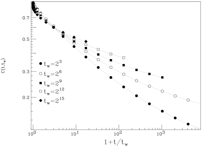
Figure 10: Double logarithmic plot of $C(t,t_{w})$ versus $1+t/t_{w}$ for the Metropolis dynamics of the infinite-dimensional $z=6$ Viana-Bray model in ($N=10^{6}$, $T=0.8=0.34T_{\mathrm{c}}$). The clearly measurable curvature indicates deviations from Eq.(9).

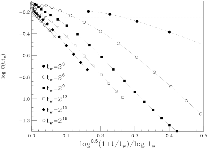
Figure 11: Logarithm of of $C(t,t_{w})$ versus $\sqrt{\log(1+t/t_{w})}/\log t_{w}$ (see Eq.(11)) for the Metropolis dynamics of the infinite-dimensional $z=6$ Viana-Bray model in ($N=10^{6}$, $T=0.8=0.34T_{\mathrm{c}}$). The dashed horizontal line is the logarithm of the $q_{\mathrm{EA}}=0.78$ [26].

The Metropolis dynamics of the infinite-dimensional $z=6$ Viana-Brey model is rather different. As we show in fig. 10, the long-time decay of $C(t,t_{w})$ is not a power-law. Thus, it cannot be fitted with Eq.(9). We have found (see fig. 11) that a fit to

$$C(t,t_{w})=S(t_{w})\exp\left[-\eta(t_{w})\frac{\sqrt{\log\left(1+t/t_{w}\right)}}{\log t_{w}}\right]\,,\ t>t_{w}.$$ (11)

is rather adequate. Moreover, $S(t_{w})$ and $\eta(t_{w})$ seem to have a well defined limit for large $t_{w}$, $S(t_{w}\to\infty)$ being quite close to the Edwards-Anderson order-parameter $q_{\mathrm{EA}}=0.78$ that in this model has been computed [26] at the one-step level of replica-symmetry breaking. If one believes that our results are almost asymptotic, so that the large $t_{w}$ correlation function truly is

$$C(t,t_{w})\approx q_{\mathrm{EA}}\exp\left[-\eta\frac{\sqrt{\log\left(1+t/t_{w}\right)}}{\log t_{w}}\right]\,,\ t>t_{w},$$ (12)

the rather amazing conclusion is reached that this ultrametric system (from the point of view of statics [3]) is not ultrametric from the point of view of dynamics! It has been pointed out [11] that dynamical ultrametricity implies (under reasonable hypothesis) statical ultrametricity, however our results suggest that dynamical ultrametricity is maybe not a necessary condition for the validity of RSB. The reader can check that the weaker property of separation of time scales holds: let $t(C;t_{w})$ be the time necessary for the correlation function at waiting-time $t_{w}$ to reach the value $C$. One has

$$\lim_{t_{w}\to\infty}\frac{t(C_{1};t_{w})}{t(C_{2};t_{w})}=0\quad\mathrm{if}\quad C_{1}>C_{2}\,.$$ (13)

It is somehow disappointing, though, that this property is expected to hold as well for the Langevin dynamics of the disordered ferromagnet [8].

4 The link overlap

Figure 12: $C_{\mathrm{link}}(t_{w},t_{w})$ and $q_{\mathrm{link}}(t_{w})$ versus $t_{w}^{-0.08}$, for the heat-bath dynamics of the 3D Edwards-Anderson model at temperatures $T=0.7T_{\mathrm{c}}$, $0.53T_{\mathrm{c}}$ and $0.44T_{\mathrm{c}}$. Lines are linear fits.

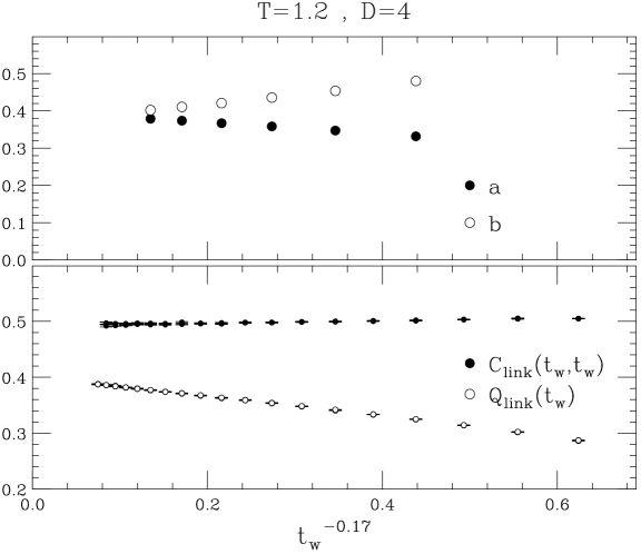
Figure 13: Top: Coefficients $a(t_{w})$ and $b(t_{w})$ (defined in Eq.(14), versus $t_{w}^{-0.17}$, for the Metropolis dynamics of the 4D Edwards-Anderson model at temperatures $T=0.6T_{\mathrm{c}}$. The fits have been performed in the window $0.1<C^{2}(t,t_{w})<0.3$. Bottom: $C_{\mathrm{link}}(t_{w},t_{w})$ and $q_{\mathrm{link}}(t_{w})$ versus $t_{w}^{-0.17}$, for the Metropolis dynamics of the 4D Edwards-Anderson model at temperatures $T=0.6T_{\mathrm{c}}$.

Figure 14: $C_{\mathrm{link}}(t,t_{w})$ versus $C^{2}(t,t_{w})$, obtained in SUE for the heat-bath dynamics of the 3D Edwards-Anderson model at $T=0.7T_{\mathrm{c}}$. The plot is restricted to the window of $C^{2}$ where a linear dependence is found for all the studied $t_{w}$. The lines are linear fits.

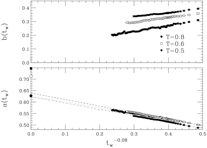
Figure 15: Top: Coefficient $b(t_{w})$, defined in Eq.(14) obtained in SUE for the heat-bath dynamics of the 3D Edwards-Anderson model versus $t_{w}^{-0.08}$, for temperatures $T=0.7T_{\mathrm{c}}$, $0.53T_{\mathrm{c}}$ and $0.44T_{\mathrm{c}}$. Bottom: As in top part, for coefficient $a(t_{w})$, defined in Eq.(14). The lines are linear fits. We also plot in the vertical axis the infinite-limit extrapolation for $C_{\mathrm{link}}(t_{w},t_{w})$ (see Fig. 12) for all three temperatures. Notice that for $T=0.8$ the infinite $t_{w}$ limit of $a(t_{w})$ and of $C_{\mathrm{link}}(t_{w},t_{w})$ seem compatible.

In recent years, a new picture of the low temperature phase of spin-glasses has been put forward [15], the so-called TNT picture. These authors propose that the link-overlap defined in Eq.(8) should have a trivial distribution function (a Dirac delta) in the thermodynamic limit (for a recent study of the link-overlap and related quantities see Ref. [27]). On the other hand, the spin-overlap defined in Eq.(7), would have a non trivial distribution function, as predicted by RSB [3]. In contradiction with RSB, the TNT picture requires that the large waiting time limit of $C_{\mathrm{link}}(t_{w},t_{w})$ be equal to the limit of $q_{\mathrm{link}}(t_{w})$ (since there would be only a possible value for this quantity!). This can be checked in our simulations. In Fig. 12 we show $C_{\mathrm{link}}(t_{w},t_{w})$ and $q_{\mathrm{link}}(t_{w})$ obtained from SUE, for temperatures $T=0.7T_{\mathrm{c}}$, $T=0.53T_{\mathrm{c}}$ and $T=0.44T_{\mathrm{c}}$, as a function of $t_{w}^{-0.08}$. The extrapolation as a function of $t_{w}^{-0.08}$ was suggested by the fact that $q_{\mathrm{link}}(t_{w})$ is roughly a linear function of this variable. Some arguments for its validity has also been given in previous work [27, 28, 24]. We notice that $q_{\mathrm{link}}(t_{w})$ has a very mild temperature dependence. Furthermore, for large $t_{w}$, $q_{\mathrm{link}}(t_{w},T=0.6)$ and $q_{\mathrm{link}}(t_{w},T=0.5)$ are on the top of each other (within error bars), while $q_{\mathrm{link}}(t_{w},T=0.8)$ is fast approaching them. Indeed, one would expect $q_{\mathrm{link}}(t_{w}=\infty,T=0.5)>q_{\mathrm{link}}(t_{w}=\infty,T=0.6)>q_{\mathrm{link}}(t_{w}=\infty,T=0.8)$, so that the three lines should cross. The fact that the infinite waiting-time limit of $q_{\mathrm{link}}(t_{w},T=0.5)$ is smaller than $q_{\mathrm{link}}(t_{w}=\infty,T=0.6)>q_{\mathrm{link}}(t_{w}=\infty,T=0.8)$, indicates that for $T=0.5$ the data should probably extrapolate like $t_{w}^{-\eta}$ with $\eta<0.08$. On the other hand, $C_{\mathrm{link}}(t_{w},t_{w})$ shows a much stronger temperature dependence and, for $T=0.5$ and $T=0.6$, is basically $t_{w}$ independent. It seems plausible that, for $T=0.8$, the limiting value of $C_{\mathrm{link}}(t_{w},t_{w})$ and $q_{\mathrm{link}}(t_{w})$ will be fairly close. However, for $T=0.5$ and $0.6$ the limits will be noticeably different unless the dynamics changes drastically at larger $t_{w}$. Interestingly enough, in four dimensions and $T=0.6T_{\mathrm{c}}$ (see Fig. 13, lower part), $C_{\mathrm{link}}(t_{w},t_{w})$ and $q_{\mathrm{link}}(t_{w})$ seems to be linear in $t_{w}^{-0.17}$, and to extrapolate to different values.

Another interesting question regards the aging properties of the link correlation-function. From the droplet [14] and TNT pictures of spin-glasses, one would not expect that $C_{\mathrm{link}}(t,t_{w})$ would age (at least, for large enough $t_{w}$). On the other hand, the RSB picture expects aging properties akin to the ones of $C(t,t_{w})$. To check for this, one could just look to $C_{\mathrm{link}}(t,t_{w})$ as a function of $C^{2}(t,t_{w})$ (see Fig. 14). If one concentrates in a small window of $C^{2}$, $0.2<C^{2}<0.35$ a linear description is perfectly adequate:

$$C_{\mathrm{link}}(t,t_{w})=a(t_{w})+b(t_{w})C^{2}(t,t_{w})\,.$$ (14)

The question now translates to the behavior of $a(t_{w})$ and $b(t_{w})$. The TNT and droplet pictures predict that $b(t_{w})$ tend to zero and $a(t_{w})$ tend to the large waiting time limit of $C_{\mathrm{link}}(t_{w},t_{w})$. On the other hand, RSB predicts a non-vanishing limit of $b(t_{w})$.

In Fig.15, we show coefficients $a(t_{w})$ (bottom) and $b(t_{w})$ (top), as a function of $t_{w}^{-0.08}$, for the heat-bath dynamics of the 3D Edwards-Anderson model, at $T=0.5,0.6$ and $0.8$. Obviously, the lower $T$, the smaller is the range of $t_{w}$ shown, because $C^{2}(t,t_{w})$ does not reach 0.2 for all the $t_{w}$ in our simulation time. The errors in $a(t_{w})$ and $b(t_{w})$ have been calculated with a Jack-Knife procedure. The coefficients seems to have a nice linear behavior in $t_{w}^{-0.08}$. One thus conclude that, unless a drastic change arise in the behavior of $a(t_{w})$ and $b(t_{w})$, the slope $b(t_{w})$ will not vanish asymptotically. This implies that $C_{\mathrm{link}}(t,t_{w})$ should age as $C^{2}(t,t_{w})$ does. One must acknowledge, however, that the conclusion is less sound for $T=0.8$ than for the lower temperatures. In fact, for $T=0.8$ the infinite-volume extrapolation of $a(t_{w})$ (see bottom part of Fig. 15) is quite close to the large time-limit of $C_{\mathrm{link}}(t_{w},t_{w})$, as TNT would predict. For the lower temperatures this extrapolations are clearly different. The data in four-dimensions support as well the RSB prediction (see the top part of Fig.13).

5 Conclusions

In this work, we report the results of a large scale Monte Carlo simulation of the heath-bath dynamics of the three dimensional Edwards-Anderson model with binary coupling at temperatures $T=0.7T_{\mathrm{c}}$, $0.53T_{\mathrm{c}}$ and $0.44T_{\mathrm{c}}$ (see table 1). The long times achieved and the large lattices studied ($60^{3}$), have been made possible by the SUE machine. In addition, shorter but more precise simulations are presented for the Metropolis dynamic of the same model in 3D, 4D and the infinite-dimensional Viana-Bray model.

For the spin correlation-function in $D=3$ and $D=4$, we find that an slightly modified power law (see Eq.(9)), well describes the data for $t>t_{w}$. This formula is identical to the cross-over like parametrization (3) proposed by Rieger et al. [20, 9]. However, in the regime $1\ll t\ll t_{w}$ a different behavior is observed. A numerical procedure is proposed for the study of the different time-sectors believed to exist in spin-glasses dynamics [8]. Indeed, a time sector with characteristic exponent $\mu=0.6$ is observed for the first time, we believe, although to firmly establish this result will require very precise simulations at still larger $t_{w}$. In spite of this, the very slow $t_{w}$ evolution of $A(t_{w})$ and $\alpha(t_{w})$ (see Eq.(9)), makes us to believe that in thermoremanent magnetization measurements (usually restricted to the range $10^{-2}t_{w}<t<10^{2}t_{w}$), a perfect full-aging behavior occurs, in agreement with a recent experiment [19], and mild disagreement with older ones [6] (see also [17]). Although it is somehow disappointing that the study of the (in)existence of more than two-time sectors in spin-glass dynamics should be restricted to simulations, we still think that it should be feasible. Nevertheless, one can always hope that new experimental techniques and protocols will be eventually able to explore this time-regime.

In infinite-dimensions, or at least for the $z=6$ Viana-Bray model, we have found a different scaling. The decay of the spin-correlation function is not a power law. Moreover, the limiting functional-form Eq.(12) is not dynamically ultrametric. Although clearly more work is needed to establish this result, it suggests that dynamical ultrametricity is maybe not such an interesting property as previously thought.

We have considered as well the aging properties of the link-overlap and the link correlation-function, both in three dimensions and in 4D. We have concluded that, unless a drastic change in the dynamical properties arises for $t_{w}$ larger than the here studied, the link correlation-function should age precisely in the same way as the spin correlation-function. This is in plain disagreement with the droplet and the TNT pictures of the spin-glass phase. However, one must acknowledge that the data at the highest studied temperature in three dimensions ($T=0.7T_{\mathrm{c}}$) are not incompatible with the TNT picture.

References

- [1] J. A. Mydosh, Spin Glasses: an Experimental Introduction (Taylor and Francis, London 1993).
- [2] K. Binder and A. P. Young, Rev. Mod. Phys. 58, 801 (1986); K. H. Fisher and J. A. Hertz, Spin Glasses (Cambridge University Press, Cambridge U.K. 1991)
- [3] M. Mézard, G. Parisi and M. A. Virasoro, Spin Glass Theory and Beyond (World Scientific, Singapore 1987); E. Marinari, G. Parisi, F. Ricci-Tersenghi, J. J. Ruiz-Lorenzo and F. Zuliani, J. Stat. Phys. 98, 973 (2000).
- [4] Spin Glasses and Random Fields, edited by A. P. Young. World Scientific (Singapore, 1997).
- [5] R.V. Chamberlin, M. Hardiman and R. Orbach, J. Appl. Phys. 52, 1771 (1983); L. Lundgren, P. Svelindh, P. Norblad and O. Beckman, Phys. Rev. Lett. 51, 911 (1983) and J. Appl. Phys. 57, 3371 (1985).
- [6] E. Vincent, J. Hamman, M. Ocio, J. P. Bouchaud and L.F. Cugliandolo in Complex behaviour of glassy systems, ed. M. Rubi, Springer-Verlag Lecture Notes in Physics 492, 184 (1997) (cond-mat/96072224).
- [7] Ph. Refregier, E. Vincent, J. Hamman and M. Ocio, J. Physique (France) 48, 1533 (1987); K. Jonason, P. Norblad, E. Vincent, J. Hamman and J. P. Bouchaud, Eur. Phys. J. B 13, 99 (2000); J.P. Bouchaud, V. Dupuis, J. Hamman and E. Vincent, Phys. Rev. B 65, 024439 (2002).
- [8] For a review see J.P. Bouchaud, L.F. Cugliandolo, J. Kurchan and M. Mézard, Out of equilibrium dynamics in Spin-Glasses and other Glassy Systems in [4].
- [9] J. Kisker, L. Santen, M. Schreckenberg and H. Rieger, Phys. Rev. B 53, 6418 (1996). For a review see H. Rieger, in Annual Reviews of Computational Physics II (World Scientific 1995, Singapore) p. 295.
- [10] J.J. Ruiz-Lorenzo, Low temperature properties of Ising spin glasses: (some) numerical simulations. To appear in ”Advances in Condensed Matter and Statistical Mechanics”, Ed. E. Korutcheva and R. Cuerno. To be published by Nova Science Publishers, preprint cond-mat/0306675.
- [11] S. Franz, M. Mézard, G. Parisi, L. Peliti, Phys. Rev. Lett. 81, 1758 (1998); J. Stat. Phys. 97, 459 (1999).
- [12] E. Marinari, G. Parisi, F. Ricci-Tersenghi and J. J. Ruiz-Lorenzo, J. Phys. A 31, 2611 (1998); S. Franz and H. Rieger, J. Stat. Phys. 79, 749 (1995).
- [13] D. Hérisson and M. Ocio, Phys. Rev. Lett. 88, 257202 (2002).
- [14] W. L. McMillan, J. Phys. C 17, 3179 (1984). A. J. Bray and M. A. Moore, in Heidelberg Colloquium on Glassy Dynamics, edited by J. L. Van Hemmen and I. Morgenstern (Springer Verlag, Heidelberg, 1986), p. 121. D. S. Fisher and D. A. Huse, Phys. Rev. Lett. 56, 1601 (1986); Phys. Rev. B 38, 386 (1988).
- [15] M. Palassini and A. P. Young, Phys. Rev. Lett. 85, 3017 (2000).
- [16] M. Picco, F. Ricci-Tersenghi and F. Ritort, Phys. Rev. B 63, 174412 (2001).
- [17] L. Berthier and J. P. Bouchaud, Phys. Rev. B 66, 054404 (2002).
- [18] A.J. Bray, Adv. Phys. 43, 357 (1994).
- [19] G.F. Rodriguez, G.G. Kenning and R. Orbach, Phys. Rev. Lett. 91, 037203 (2003).
- [20] H. Rieger, J. Phys. A26, L615 (1993).
- [21] J. Pech, A. Tarancón and C. L. Ullod, Comput. Phys. Commun. 106, 10 (1997).
- [22] J. J. Ruiz-Lorenzo and C. L. Ullod. Comput. Phys. Commun. 125, 210 (2000).
- [23] A. Cruz, J. Pech, A. Tarancón, P. Téllez, C. L. Ullod, C. Ungil, Comput. Phys. Commun. 133, 165 (2001).
- [24] E. Marinari, G. Parisi, F. Ricci-Tersenghi and J.J. Ruiz-Lorenzo, J. Phys. A 33, 2373 (2000).
- [25] H.G. Ballesteros, A. Cruz, L.A. Fernandez, V. Martin-Mayor, J. Pech, J.J. Ruiz-Lorenzo, A. Tarancon, P. Tellez, C.L. Ullod and C. Ungil, Phys. Rev. B 62, 14237 (2000).
- [26] M. Mézard and G. Parisi, Eur. Phys. J. B 20, 217 (2001).
- [27] E. Marinari, G. Parisi and J.J. Ruiz-lorenzo, J. of Phys. A: Math. and Gen. 35, 6805 (2002).
- [28] E. Marinari, G. Parisi and J.J. Ruiz-lorenzo, Phys. Rev. B 58, 14852 (1998); E. Marinari, G. Parisi F. Ritort and J.J. Ruiz-lorenzo, Phys. Rev. Lett. 76, 843 (1996).