Fermi-Bose Correspondence and Bose-Einstein Condensation in The Two-Dimensional Ideal Gas

Abstract

The ideal uniform two-dimensional (2D) Fermi and Bose gases are considered both in the thermodynamic limit and the finite case. We derive May’s Theorem, viz. the correspondence between the internal energies of the Fermi and Bose gases in the thermodynamic limit. This results in both gases having the same heat capacity. However, as we shall show, the thermodynamic limit is never truly reached in two dimensions and so it is essential to consider finite-size effects. We show in an elementary manner that for the finite 2D Bose gas, a pseudo-Bose-Einstein condensate forms at low temperatures, incompatible with May’s Theorem. The two gases now have different heat capacities, dependent on the system size and tending to the same expression in the thermodynamic limit.

I Introduction

Since their inception into the theoretical framework of physics, much work has been carried out on both the Fermi-Dirac as well as the Bose-Einstein distributions Huang (1987); Pathria (1996). Much of this focuses on the behaviour of fermions and bosons at low temperatures, where the deviations in their behaviour arising from the distributions are significant and quantum effects dominate. The advent of comprehensive experimental techniques for lowering the temperature of systems to previously theoretical values over the last few decades has contributed significantly to this and revealed a wealth of unusual behaviour at extremely low temperatures, in particular the unusual phenomenon of Bose-Einstein condensation - a macroscopic occupation of the ground state of a gas of bosons at finite temperature.

For most of this time, however, there has been only a cursory and passing interest in low-dimensional Fermi and Bose systems. This has been mainly because they have been viewed as little more than abstract theoretical and mathematical constructs. Moreover, it was felt that there was little behaviour of interest to be found in these lower dimensions. It is only over the last couple of decades that there has been a growing interest in the properties of gases obeying the Fermi and Bose distributions in lower dimensions. This has been driven by firstly, the growing practical importance of low-dimensional systems, such as for example in computers, as well as new experimental techniques (such as, for example, 2D adsorbed systems, in particular, 2D adsorbed helium films Lusher et al. (1991); Siqueira et al. (1993); Casey et al. (1998); Ray et al. (1998)) that raise the possibility of being able to trap and study low-dimensional quantum systems. Typical systems being studied include superfluid and superconducting films, quantum Hall and related two-dimensional electron gases and low-dimensional trapped Bose gases. Further, the renewed theoretical interest in low-dimensional physics over the last couple of decades has led to a growing realisation that these systems possess equally fascinating and unique quantum behaviour of their own (see, for example, Ref. Schakel, 1998). In particular, recent observations of exotic quantum behavior, such as Bose-Einstein condensation (BEC) Anderson et al. (1995); Bradley et al. (1997); Davis et al. (1995) and Fermi degeneracy DeMarco and Jin (1999), in three-dimensional systems have led to a growing interest in lower-dimensional systems.

One special theoretical interest in the 2D ideal gas is due to the fact that we can obtain completely analytic expressions for the chemical potential $\mu$ and other thermodynamic properties. This arises, in part, from the energy-independence of the 2D density of states within the semi-classical approximation. Furthermore, in two dimensions, there is an unusual correspondence between the Bose and Fermi cases, first noted by May May (1964) and subsequently, explored further in later papers Mullin and Fernandez (2003); Toda et al. (1983); Aldrovandi (1992); Viefers et al. (1995); Lee (1997).

In his seminal paper May (1964), May noted the unexpected result that the thermal capacities of the ideal 2D Bose and Fermi gases are identical in the thermodynamic limit, i.e. their internal energies differ only by a constant temperature-independent amount. This only holds in the thermodynamic limit, or equivalently, the semi-classical approximation that the energy level spacing is negligible compared with the temperature T, allowing us to replace the discrete (quantum) structure by a continuum. Real-world systems, however, are always finite, typically of the order of $10^{3}-10^{6}$ particles for trapped gases, and more for adsorbed systems. Moreover, as we shall see later, the chemical potential $\mu$ has a logarithmic dependence on the total number of particles $N$ in the system. Thus, the thermodynamic limit is never truly reached in two dimensions and is an abstract theoretical construct, making it essential to consider finite-size effects. These may be experimentally significant, and lead to deviations from May’s Theorem.

In the following sections, we shall consider the behaviour of the uniform 2D ideal Bose and Fermi gases. In the next section, we shall briefly outline the gases in the thermodynamic limit and derive May’s Theorem before examining the Bose and Fermi gases for a finite number of particles in Section III. Though there is no BEC in the thermodynamic limit, we will demonstrate that there is a pseudo-condensation at very low temperatures for the finite 2D Bose gas. This is then used to show in Section IV that the finite-size effects lead to differing heat capacities for the Bose and Fermi gases, and a breakdown in May’s Theorem for gases with a finite number of particles. Further, the inadequacy of heat capacities as a means of determining phase transitions is discussed.

II The Thermodynamic Limit

As the 2D ideal gas and May’s Theorem have already been examined at length before in the thermodynamic limitMay (1964); Mullin and Fernandez (2003); Toda et al. (1983); Aldrovandi (1992); Viefers et al. (1995); Lee (1997), we shall simply draw on earlier approaches to provide a brief overview. Consider $N$ free and identical particles of mass $m$ in a 2D box of ‘volume’$A$, with rigid-box boundary conditions. The energy values for an arbitrary particle then are

$$\varepsilon_{i}=\frac{\hbar^{2}k^{2}}{2m},\qquad k^{2}=\frac{\pi^{2}}{A}\left(n^{2}_{x}+n^{2}_{y}\right),$$ (1)

where $k$ is the momentum characterising the energy states $\varepsilon_{i}$, $i,n_{x},n_{y}=1,2,3\ldots$ and $(n_{x},n_{y})$ are points in the positive quadrant of a unit square lattice. In the thermodynamic limit, the ground state energy tends to 0. For a finite system, however, due to the Heisenberg uncertainty principle, this is always greater than 0, as $\left(n_{x},n_{y}\right)=\left(1,1\right)$. So, for simplicity, we shift the energy scale, taking the ground state energy as 0,

$$\varepsilon_{i}=\frac{\hbar^{2}k^{2}}{2m}-\varepsilon_{0}=\frac{\pi^{2}\hbar^{2}}{2mA}\left(n^{2}_{x}+n^{2}_{y}-2\right).$$ (2)

Assuming that the system is in thermal equilibrium at temperature $T$ and chemical potential $\mu$, then the mean number of particles $n\left(\varepsilon_{i}\right)$ at a given energy $\varepsilon_{i}$ is given by

$$n\left(\varepsilon_{i}\right)=\frac{1}{e^{\left(\varepsilon_{i}-\mu\right)/{k_{B}T}}\pm 1}.$$ (3)

Here and later, the upper (lower) signs are for fermions (bosons). The total number of particles N and the internal energy E of the system are now given by

$$N=\sum_{i=1}^{\infty}n\left(\varepsilon_{i}\right),$$ (4)

$$E=\sum_{i=1}^{\infty}\varepsilon_{i}n\left(\varepsilon_{i}\right).$$ (5)

where the sum is taken over the single particle energy states. In the semiclassical approximation, we assume that the spacing between the energy levels of the particle states is negligible. This allows us to replace the sum with an integral over energy states using the density of states $g(\varepsilon)$ and the spin degeneracy $\alpha$,

$$f=\alpha\int_{0}^{\infty}f\left(\varepsilon\right)g\left(\varepsilon\right)n\left(\varepsilon\right)d\varepsilon,$$ (6)

where $f\left(\varepsilon\right)$ is a general single-particle function of energy. However, this approximation is only exact in the thermodynamic limit when the system size is infinite, and at very high temperatures $T$. As we shall see in Section III, for finite systems at low T, these assumptions are invalid and the discreteness of the energy levels cannot be ignored. In other words, we will be at a temperature $T$ below which the semiclassical approximation breaks down and modifications need to be made. However, it may be possible to compensate by modifying the semi-classical approximation to allow for finite-size effects.

We now evaluate the various thermodynamic quantities for arbitrary spin, i.e. arbitrary $\alpha$, for both the 2D Fermi and Bose gases in the thermodynamic limit. In 2D, $g(\varepsilon)$ and thereby, the Fermi energy $\varepsilon_{F}$ are given by,

$$g(\varepsilon)=\frac{mA}{2\pi\hbar^{2}},\qquad\varepsilon_{F}=\frac{2\pi\hbar^{2}N}{\alpha mA}.$$ (7)

For comparison, we adopt $\varepsilon_{F}$ as a characteristic energy $\varepsilon_{C}$ for the Bose gas also, allowing us to express later results in a unified form. In 2D, as $g(\varepsilon)$ is a constant, we have a simple integral for N,

$$N=\frac{\alpha mA}{2\pi\hbar^{2}}\int_{0}^{\infty}\frac{d\varepsilon}{e^{\left(\varepsilon-\mu\right)/{k_{B}T}}\pm 1}.$$ (8)

This may be expressed using the Fermi-Dirac and Bose-Einstein functions Huang (1987); Pathria (1996), $f_{\nu}(z)$ and $g_{\nu}(z)$ respectively,

$$f_{\nu}\left(z\right)=\frac{1}{\Gamma\left(\nu\right)}\int_{0}^{\infty}\frac{x^{\nu-1}dx}{z^{-1}e^{x}+1}$$ (9)

$$g_{\nu}\left(z\right)=\frac{1}{\Gamma\left(\nu\right)}\int_{0}^{\infty}\frac{x^{\nu-1}dx}{z^{-1}e^{x}-1},$$ (10)

where $\Gamma\left(\nu\right)$ is the Euler gamma function. These can also be expressed using the polylogarithmic functions $\textnormal{Li}_{\nu}(z)$ Abramowitz and Stegun (1964); Lewin (1958),

$$f_{\nu}\left(z\right)=-\textnormal{Li}_{\nu}\left(-z\right),$$ (11)

$$g_{\nu}\left(z\right)=\textnormal{Li}_{\nu}\left(z\right).$$ (12)

For N above, $\nu=1$ and $z$ is the fugacity ($z=e^{\mu/k_{B}T}$). Solving (8) in terms of $\varepsilon_{C}$ and rearranging, we can now express the fugacity $z$ and thereby, the chemical potential $\mu$ as a completely analytic expression

$$z_{F,B}=e^{{\mu}/{k_{B}T}}=\mp\left(1-e^{\pm{\varepsilon_{C}}/{k_{B}T}}\right),$$ (13)

where $z_{F}$ ($z_{B}$) is the fugacity for the ideal Fermi (Bose) gas. As $T\rightarrow 0$, $z_{B}$ smoothly approaches 1. Denoting the fugacity $z_{B}$ by $z_{B}=e^{-\alpha}$, as $z_{B}\rightarrow 1$,

$$g_{1}\left(e^{-\alpha}\right)=-\ln\left(1-e^{-\alpha}\right)\underset{\alpha\rightarrow 0}{\longrightarrow}-\ln\alpha.$$ (14)

N diverges logarithmically as $\alpha\rightarrow 0$. Thus, it has no upper bound, and there is no temperature below which the ground state can be said to be macroscopically occupied in comparison to the excited states. Thus, there is no BEC in the thermodynamic limit. This is a qualification of the oft-paraded statement that there is no BEC for $D\leq 2$, where $D$ is the number of dimensions. However, as we shall see in Section III, the logarithmic divergence implies that at sufficiently low T, bosons still crowd into low-lying states to give a pseudo-condensate.

The internal energy may be similarly solved,

$$E_{F}=Nk_{B}T\left(\frac{k_{B}T}{\varepsilon_{C}}\right)f_{2}\left(e^{{\varepsilon_{C}}/{k_{B}T}}-1\right),$$ (15)

$$E_{B}=Nk_{B}T\left(\frac{k_{B}T}{\varepsilon_{C}}\right)g_{2}\left(1-e^{{-\varepsilon_{C}}/{k_{B}T}}\right).$$ (16)

Now, using the following property of the dilogarithmic functionMay (1964); Lewin (1958) $\textnormal{Li}_{2}\left(x\right)$,

$$f_{2}\left(\frac{1}{x}-1\right)=g_{2}\left(1-x\right)+\frac{1}{2}\left(\ln x\right)^{2},$$ (17)

we can easily show

$$E_{F}=E_{B}+\frac{1}{2}N\varepsilon_{C}.$$ (18)

i.e. for all $T$, $E_{B}$ differs from $E_{F}$ by a constant temperature independent energy, which does not contribute to the heat capacity. This gives May’s Theorem May (1964), which states that the heat capacities of the ideal 2D Fermi and Bose gases are identical at all T and N,

$$C_{V,Bose}=\frac{\partial E_{B}}{\partial T}|_{{}_{V}}=\frac{\partial E_{F}}{\partial T}|_{{}_{V}}=C_{V,Fermi}.$$ (19)

The above result indicates that the 2D ideal Bose gas does not undergo a phase transition, as any experimental measurement of the heat capacity would be the same as for a 2D Fermi gas, and would lack the characteristic bump that indicates the presence of BEC in the 3D Bose gas. However, as we shall see, this is because we have failed to consider the finite nature of any real systems.

III The Finite Gas

The case of the finite ideal Bose gas in two dimensions has already been considered to varying degrees in earlier papers Osborne (1949); Ziman (1953); Mills (1964); Goble and Trainor (1967); Chester (1968); Krueger (1968); Irnry (1969); Barber (1983); Grossmann and Holthaus (1995), and more recently, by Pathria Pathria (1998). Most have commented that it may be possible to have a pseudo-condensation in the Bose gas in two dimensions, with the transition temperature typically going as $T_{C}\sim 1/\ln{N}$. Here, we present a simpler and more comprehensive analysis of the problem that not only offers far more insight into how the finite size of the system leads to the breakdown of May’s Theorem and a pseudo-condensation in the Bose gas, but further, in Section IV, discusses how the heat capacities for the Fermi and Bose gases differ for finite systems, and how such a pseudo-condensation may be experimentally measured.

At $T=0$, the 2D Bose gas is in its ground state, and we have the trivial case of ground state macroscopic occupation. Extrapolating, however, a range of finite temperatures must exist near $T=0$, which may depend on $N$, where the number of particles in the ground state is also of $O\left(N\right)$ - a macroscopic occupation. At very low $T$, this can be a significant fraction of $N$, and the semi-classical approach is now flawed as $N$ is no longer continuous. Taking macroscopic occupation of the ground state as the defining characteristic of BEC, we consider the ground state separately analogous to standard treatments of the 3D Bose gas Huang (1987); Pathria (1996). For finite systems, the discrete level structure requires us to introduce a cutoff energy at the first excited level $\varepsilon_{1}$. The integral is now bounded and we can remove the logarithmic divergence. Thus, we can have a pseudo-BEC in a finite two-dimensional system. This must be associated with a breakdown of May’s theorem at sufficiently low $T$ for finite systems. We thus write (8) for the Bose gas as

$$N=N_{0}+\frac{\alpha mA}{2\pi\hbar^{2}}\int_{\varepsilon_{1}}^{\infty}\frac{d\varepsilon}{e^{{\left(\varepsilon-\mu\right)}/{k_{B}T}}-1},$$ (20)

It should be noted that the above approximation is quite a simple and crude one, as it is only the leading term of the Euler-Maclaurin summation formula. However, it suits the purposes of our paper as our intention here is merely to highlight how even the simplest approximations show that there is a pseudo-condensation in the finite Bose gas. A more detailed approximation will only lead to minor modifications to the core results presented in the rest of this paper. Further, the leading correction term to the integral above in the Euler-Maclaurin expansion is of the order of $N_{1}=n\left(\varepsilon_{1}\right)=\left(e^{\left(\varepsilon_{1}-\mu\right)/k_{B}T}\right)^{-1}$. Taking the ratio $N_{0}/N_{1}$ of the number of particles in the ground state to that in the first excited state, we can see

$$\frac{N_{0}}{N_{1}}\approx\frac{\varepsilon_{1}-\mu}{-\mu}$$ (21)

As the chemical potential $\mu$ for the 2D Bose gas is always negative and less than $0$, the above ration is always greater than 1. Further, as $T\rightarrow 0$, $\mu\rightarrow 0$ and the above expression clearly goes to $\infty$. Further, a more detailed evaluation of (21) gives us

$$\frac{N_{0}}{N_{1}}\approx\frac{3\pi^{2}\hbar^{2}}{2mAk_{B}T}e^{\frac{2\pi\hbar^{2}N}{\alpha mAk_{B}T}}$$ (22)

This clearly rapidly goes to infinity as both the temperature $T$ as well as the number of particles $N$ increase. Moreover, for the regime in question, we are interested in very low temperatures where from the above equation (22), the ratio $N_{0}/N_{1}$ is clearly significantly large.

Thus, we are justified in making our crude approximation and denoting the number of particles $N$ by (20) above. Solving as before, we now have

$$N-N_{0}=-\frac{\alpha mAk_{B}T}{2\pi\hbar^{2}}\ln\left(1-z_{B}e^{{-3\pi^{2}\hbar^{2}}/{2mAk_{B}T}}\right)$$ (23)

and $\varepsilon_{1}$ prevents the logarithmic divergence. This is because the excited states cannot accommodate all the particles at low $T$, and the excess are forced into the ground state, leading to a pseudo-BEC. Equivalently, changing variables $\varepsilon\rightarrow\varepsilon+\varepsilon_{1}$ and resetting the integral from zero, we may also express (20) in terms of the Bose-Einstein functions $g_{\nu}\left(z\right)$ as

$$N-N_{0}=\frac{\alpha mAk_{B}T}{2\pi\hbar^{2}}g_{1}\left(z_{B}e^{{-3\pi^{2}\hbar^{2}}/{2mAk_{B}T}}\right).$$ (24)

Thus, we now have an effective fugacity

$$z_{B}\longrightarrow z_{B}^{\prime}=z_{B}e^{{-3\pi^{2}\hbar^{2}}/{2mAk_{B}T}}$$

$$=e^{{-3\alpha\pi\varepsilon_{C}}/{4Nk_{B}T}}\left(1-e^{{-\varepsilon_{C}}/{k_{B}T}}\right).$$ (25)

where $z_{B}$ is as before. This summarizes the finite-size effects on the Bose gas. The extra term is dependent on the system size and tends to 1 as $N\rightarrow\infty$. For finite $N$ and low $T$, it is less than 1, and so, the fugacity is modified. Thus, there is a pseudo-BEC here but none in the thermodynamic limit. This macroscopic occupation is a purely boson phenomenon, and so, the behaviour will be markedly different from that of the two-dimensional Fermi gas.

For the Fermi gas, Pauli’s principle forbids macroscopic occupation of any state. Thus, the first term is not divergent. $z_{F}$ (Eq. (13)) still holds, and finite-size effects only appear for the Bose gas, where the excited states take as many particles as possible at low $T$, with the excess forced into the ground state. This occurs at the maximal value of the fugacity $z_{B}=1$. Thus, we can define a characteristic temperature $T_{C}$ that marks the onset of condensation where $N_{0}\approx 0$ and $z\approx 1$,

$$N\cong-\frac{\alpha mAk_{B}T_{C}}{2\pi\hbar^{2}}\ln\left(1-e^{{-3\pi^{2}\hbar^{2}}/{2mAk_{B}T_{C}}}\right)$$

$$\simeq\frac{Nk_{B}T_{C}}{\varepsilon_{C}}\ln\left(\frac{4Nk_{B}T_{C}}{3\pi\alpha\varepsilon_{C}}\right)$$ (26)

for very low $T$. We may solve (26) to give

$$T_{C}=\frac{\varepsilon_{C}}{k_{B}}\frac{1}{W\left({4N}/{3\pi\alpha}\right)},$$ (27)

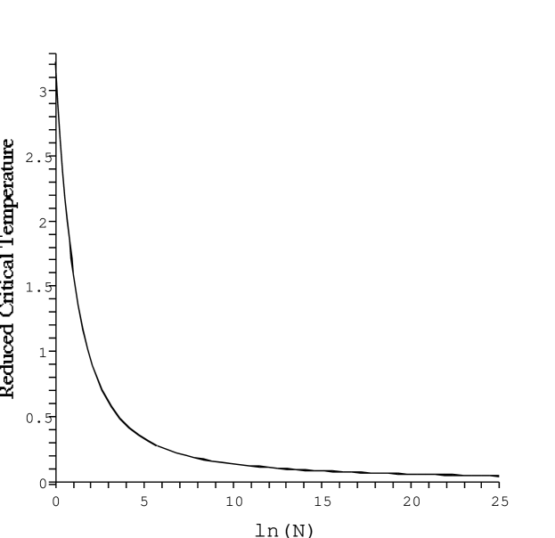
Figure 1: Plot of reduced characteristic condensation temperature $k_{B}T_{C}/\varepsilon_{C}$ against number of particles $N$ in the system. [N.B. Spin degeneracy $\alpha=1$]

where, $W\left(x\right)$ is the Lambert function Corless et al. (1996) and is the principal solution for $w$ in the equation $x=we^{w}$. This is plotted in Fig. 1. It may be viewed as a generalisation to a logarithm. Thus, our result (27) is a refinement of the earlier noted result that the transition temperature behaves like $T_{C}\sim 1/\ln{N}$. As $N\rightarrow\infty$, the reduced characteristic temperature ${k_{B}T_{C}}/{\varepsilon_{C}}\rightarrow 0$. Thus, in the thermodynamic limit, we recover the conventional result that there is no BEC in two dimensions. The condensate fraction is

$$\frac{N_{0}}{N}\cong 1-\frac{k_{B}T}{\varepsilon_{C}}\ln\left(\frac{4Nk_{B}T}{3\pi\alpha\varepsilon_{C}}\right)$$

$$\cong 1-\frac{T}{T_{C}}\left[1+\frac{k_{B}T_{C}}{\varepsilon_{C}}\ln\left(\frac{T}{T_{C}}\right)\right].$$ (28)

This only holds for very low temperatures $T<T_{C}$. As can be seen in Fig. 2, the condensate occurs at lower and lower $T$ as the system size $N$ increases. In the thermodynamic limit, there is no BEC at all.

Having shown the pseudo-condensation, we now move on to consider how the Fermi-Bose correspondence predicted by May is affected when the gases are assumed finite.

IV The Finite Gas: Internal Energy and Heat Capacity

The internal energies may be similarly found. The first term in (5) for the Bose gas is divergent as it is the internal energy $E_{gs}$ associated with the anomalously large ground state. Separating this out,

$$E_{B}=E_{gs}+\sum_{i=1}^{\infty}\frac{\varepsilon_{i}}{e^{\left(\varepsilon_{i}-\mu\right)/{k_{B}T}}-1},$$ (29)

As we have set $E_{gs}$ as the zero-point energy, the first term is 0. Changing variables $\varepsilon\rightarrow\varepsilon+\varepsilon_{1}$, and converting to an integral,

$$E_{B}=\frac{N}{\varepsilon_{C}}\int_{0}^{\infty}\frac{\varepsilon+\varepsilon_{1}}{e^{\left(\varepsilon+\varepsilon_{1}-\mu\right)/{k_{B}T}}-1}d\varepsilon$$

$$=\frac{N}{\varepsilon_{C}}\left(k_{B}T\right)^{2}g_{2}\left(z_{B}^{\prime}\right)+\frac{\varepsilon_{1}}{\varepsilon_{C}}Nk_{B}Tg_{1}\left(z_{B}^{\prime}\right).$$ (30)

where $z_{B}^{\prime}$ is defined by (25). We again have an effective fugacity $z_{B}^{\prime}$ and additional terms, which are negligible in the thermodynamic limit. By contrast, for the finite Fermi gas, there is no divergence in the ground state term, and we have the same expression for the fugacity (13) as before. The internal energies of the finite two-dimensional Fermi and Bose gases are then given by

$$E_{F} = Nk_{B}T\left(\frac{k_{B}T}{\varepsilon_{C}}\right)f_{2}\left(e^{{\varepsilon_{C}}/{k_{B}T}}-1\right)$$ (31)

$$E_{B} = \left(\frac{Nk_{B}^{2}T^{2}}{\varepsilon_{C}}\right)g_{2}\left(z_{B}^{\prime}\right)-\frac{3\pi\alpha}{4}k_{B}T\ln\left(1-z_{B}^{\prime}\right)$$ (32)

Eq. (18) is no longer true, as we cannot simply express $E_{F}$ in terms of $E_{B}$ as before. $E_{B}$ now has additional $T$-dependent terms that lead to a differing heat capacity.

May’s Theorem is thus a special limiting case for the 2D Bose and Fermi internal energies in the thermodynamic limit. Here, the additional factor $e^{{-3\pi\alpha\varepsilon_{C}}/{4Nk_{B}T}}$ tends to unity in the thermodynamic limit, recovering May’s Theorem. The same occurs in the high $T$ limit for a finite gas as above $T_{C}$, there is no macroscopic ground state occupation. Thus, above $T_{C}$, we may approximate the internal energies by (15) and (16) with differences becoming marked only at very low $T$ and/or very small system size $N$.

We now calculate the Bose and Fermi heat capacities by using the following polylogarithmic identity Pathria (1996); Abramowitz and Stegun (1964),

$$\frac{d}{dz}Li_{n+1}\left(z\right)=\frac{1}{z}Li_{n}\left(z\right)$$ (33)

The heat capacity for the finite gas is then given by

$$C_{V,Fermi}=\frac{Nk_{B}^{2}}{\varepsilon_{C}}\left[2Tg_{2}\left(1-e^{{-\varepsilon_{C}}/{k_{B}T}}\right)-\frac{\varepsilon_{C}^{2}}{k_{B}^{2}T}\frac{1}{e^{{\varepsilon_{C}}/{k_{B}T}}-1}\right]$$ (34)

$$C_{V,Bose}=\frac{Nk_{B}^{2}}{\varepsilon_{C}}\left[2Tg_{2}\left(z_{B}^{\prime}\right)+\frac{\varepsilon_{C}}{k_{B}}\frac{\ln\left(1-z_{B}^{\prime}\right)}{e^{{\varepsilon_{C}}/{k_{B}T}}-1}\right]$$

$$+\frac{3\pi\alpha k_{B}}{16N}\left[\frac{\varepsilon_{C}\left(3\pi\alpha z_{B}^{\prime}-4Ne^{-{\varepsilon_{C}}/{k_{B}T}-{3\alpha\pi\varepsilon_{C}}/{4Nk_{B}T}}\right)}{k_{B}T\left(1-z_{B}^{\prime}\right)}-8N\ln\left(1-z_{B}^{\prime}\right)\right]$$ (35)

The Bose heat capacity $C_{V,Bose}$ now contains several terms dependent on both $N$ and $T$. It should also be noted that the last two terms in the heat capacity are very much smaller than the first two terms and become increasingly negligible as the system size increases. At high $T$ and/or very large $N$, the additional terms tend to zero, i.e. as $N\rightarrow\infty$ and/or $T\rightarrow\infty$, ${\pi\alpha\varepsilon_{C}}/{Nk_{B}T}\rightarrow 0$, and (35) reduces to the standard expression in the thermodynamic limit,

$$C_{V,Bose}\rightarrow\frac{2Nk_{B}^{2}T}{\varepsilon_{C}}g_{2}\left(1-e^{{-\varepsilon_{C}}/{k_{B}T}}\right)-\frac{N\varepsilon_{C}}{T}\frac{1}{e^{{\varepsilon_{C}}/{k_{B}T}}-1}=C_{V,Fermi}.$$ (36)

This is one of the most important results of our paper, and shows clearly that May’s theorem arises as the thermodynamic limit of (34) and (35), when the heat capacities of the Bose and Fermi gases become equal. Nevertheless, for most real-world 2D systems, above the characteristic temperature $T_{C}$, which marks the onset of Bose-Einstein condensation in the two-dimensional ideal Bose gas, ${\pi\alpha\varepsilon_{C}}/{Nk_{B}T}$ is very small and so, even for finite gases, the thermal capacities of the Bose and Fermi systems are approximately equal above the condensation temperature.

In Fig. 3, we plot the reduced heat capacities (${C_{V}}/{Nk_{B}T^{*}}$) for the Fermi and Bose gases against the reduced temperature $T^{*}$(where $T^{*}={k_{B}T}/{\varepsilon_{C}}$) for varying system size $N$, using the full expression for both $C_{V,Bose}$ and $C_{V,Fermi}$. As the heat capacity is approximately linear close to $T=0$ in the thermodynamic limit, we would expect the plots for the 2D Fermi gas to tend to a horizontal line as $T\rightarrow 0$. This limiting value will be at the critical value when $T^{*}=0$, i.e.

$$\frac{C_{V,Fermi}}{Nk_{B}T^{*}}=2g_{2}\left(1\right)=2\zeta\left(2\right)=\frac{\pi^{2}}{3}.$$ (37)

In contrast, for the finite 2D Bose gas, we expect to see a deviation from the above mentioned low-temperature behaviour. In particular, we expect that the reduced heat capacity (${C_{V}}/{Nk_{B}T^{*}}$) will fall to 0 following the formation of the condensate. Our plots indicate distinct differences between the reduced heat capacities for the Bose and Fermi gases, particularly at very low $T$ in the vicinity of and below the condensation temperature $T_{C}$. Then, $C_{V,Bose}$ is less than $C_{V,Fermi}$ and starts to deviate significantly around $T_{C}$, before rapidly going to zero as we approach $T=0$. This is in marked contrast to the 3D Bose gas, where the conventional heat capacity $C_{V}/Nk_{B}$ peaks at some finite $T$. In the two-dimensional case, however, the heat capacity $C_{V}/Nk_{B}$ is a smooth function of $T$, in keeping with the size-dependent nature of the condensation. Here, instead, we see a “bump”in the plot for the reduced heat capacity ${C_{V}}/{Nk_{B}T^{*}}$ of the 2D Bose gas, indicating the presence of a condensation. Further, as N increases, the behaviour tends to that of the 2D Fermi gas as the condensation forms at lower temperatures, and consequently, the fall-off of the reduced heat capacity occurs at lower temperatures. Indeed, with $N=500000$, the two plots of the Fermi and Bose gases are virtually indistinguishable. This is significant as conventionally, the heat capacity $C_{V}/Nk_{B}$ is used experimentally to determine if a Bose-Einstein condensation has occurred. However, as can be seen from above, the heat capacity does not necessarily peak for a weak transition which is dependent on the system size, and we have to examine alternate expressions to determine the presence of a condensation.

V Discussion and Conclusion

In this paper, we set out to discuss the two-dimensional ideal Bose and Fermi gases in the absence of any trapping potentials, and both in the thermodynamic limit and the finite case. In particular, we were interested in May’s Theorem, and its breakdown for finite systems.

As can be seen above in Sections III and IV, the 2D finite Fermi system displays the same behaviour as in the thermodynamic limit but the Bose gas deviates significantly for a finite system and undergoes a pseudo-Bose-Einstein condensation. It is not a “true”condensation as for the 3D Bose gas, where there is a distinct phase transition in the thermodynamic limit and a peak in the heat capacity. Rather, here we have a characteristic condensation temperature $T_{C}$ that is dependent on the system size and tends to zero in the thermodynamic limit. Moreover, though these is no heat capacity peak here, it still deviates significantly from the Fermi heat capacity below $T_{C}$ with the deviations tending to zero as the system size and/or the temperature increase. In other words, we have a peak in the reduced heat capacity, as shown in Fig. 3. This raises the question of what exactly is defined as a phase transition. The two-dimensional Bose gas undergoes a significant change at low temperatures but only in the finite case. Thus, it is not what may be termed a “conventional”phase transition as for the three-dimensional Bose gas, since it ceases to exist in the thermodynamic limit. However, from an experimental perspective, a system is never truly in the thermodynamic limit, and so, what we have termed a “pseudo-condensation”is expected. This also, therefore, casts doubt on the use of the heat capacity as a means of identifying phase transitions, as discussed above.

As a final note, we would like to consider some of the outstanding problems. The above analysis is a simple one and deals with only the ideal two-dimensional gas. There is still considerable debate whether such behaviour is to be found for an interacting two-dimensional gas. Some authorsPetrov et al. (2000) have claimed that there is a true condensation for the finite interacting 2D system at sufficiently low temperatures as the coherence length becomes larger than the condensate size. Others, however, have claimed that any phase transition would disappear in the presence of particle interactionsMullin (1997), as predicted by the Hohenberg theorem. Clearly, the presence of interactions will modify our results greatly. As yet, however, there is no indication if there is any correspondence between the two-dimensional Fermi and Bose gases, when they are interacting, and further, if a pseudo-condensation is to be found for the finite Bose gas. Further, similar analogues exist in other dimensions for ideal gases in a trapping potentialKetterle and van Druten (1996); Mullin (1997). It would be interesting to debate whether there are deeper implications due to the Fermi-Bose correspondence, and where such an situation occurs, it is a special unique case. This is an area of active work, with new experimental innovations making the resolution of the above problems and the elucidation of two-dimensional gases only a matter of time now.

Figure 2: Plot of condensate fraction $N_{0}/N$ against reduced temperature $k_{B}T/\varepsilon_{C}$ for (from right to left) $N$ = $10^{3}$, $10^{4}$, $10^{5}$, $10^{6}$, $10^{9}$, $10^{50}$. [$\alpha=1$]

Figure 3: Plot of difference in the reduced heat capacities $C_{V}/Nk_{B}T^{*}$ of the Fermi and Bose gases against reduced temperature $T^{*}=k_{B}T/\varepsilon_{C}$ for (from top to bottom) $N$ = : 500, 5000, 50000, 500000. [$\alpha=1$]

References

- Huang (1987) K. Huang, Statistical Mechanics (John Wiley and Sons, New York, 1987), 2nd ed.
- Pathria (1996) R. K. Pathria, Statistical Mechanics (Butterworth-Heinemann, Oxford, 1996), 2nd ed.
- Lusher et al. (1991) C. P. Lusher, J. Saunders, and B. P. Cowan, Physical Review Letters 67, 2199 (1991).
- Siqueira et al. (1993) M. Siqueira, C. P. Lusher, B. P. Cowan, and J. Saunders, Physical Review Letters 71, 1407 (1993).
- Casey et al. (1998) A. Casey, H. Patel, J. Nyeki, B. P. Cowan, and J. Saunders, Journal of Low Temperature Physics 113, 293 (1998).
- Ray et al. (1998) R. Ray, J. Nyeki, B. P. Cowan, and J. Saunders, Physical Review Letters 81, 152 (1998).
- Schakel (1998) A. M. J. Schakel (1998), eprint cond-mat/990867.
- Anderson et al. (1995) M. H. Anderson, J. R. Ensher, M. R. Matthews, C. E. Wieman, and E. A. Cornell, Science 269, 198 (1995).
- Bradley et al. (1997) C. C. Bradley, C. A. Sackett, and R. G. Hulet, Physical Review Letters 78, 985 (1997).
- Davis et al. (1995) K. B. Davis, M.-O. Mewes, M. R. Andrews, N. J. van Druten, D. S. Durfee, D. M. Kurn, and W. Ketterle, Physical Review Letters 75, 3969 (1995).
- DeMarco and Jin (1999) B. DeMarco and D. S. Jin, Science 285, 903 (1999).
- May (1964) R. M. May, Physical Review 135, A1515 (1964).
- Mullin and Fernandez (2003) W. J. Mullin and J. P. Fernandez, American Journal of Physics 71, 661 (2003).
- Toda et al. (1983) M. Toda, R. Kubo, and N. Saito, Statistical Physics I (Springer Verlag, Berlin, 1983).
- Aldrovandi (1992) R. Aldrovandi, Fortschritte der Physik 40, 631 (1992).
- Viefers et al. (1995) S. Viefers, F. Ravndal, and T. Haugset, American Journal of Physics 63, 369 (1995).
- Lee (1997) M. Lee, Physical Review E 55, 1518 (1997).
- Abramowitz and Stegun (1964) M. Abramowitz and I. A. Stegun, Handbook of Mathematical Functions (National Bureau of Standards, Washington DC, 1964).
- Lewin (1958) L. Lewin, Dilogarithms and Associated Functions (McDonald, London, 1958).
- Osborne (1949) M. F. M. Osborne, Physical Review 76, 396 (1949).
- Ziman (1953) J. M. Ziman, Philosophical Magazine 44, 548 (1953).
- Mills (1964) D. L. Mills, Physical Review 134, A306 (1964).
- Goble and Trainor (1967) D. F. Goble and L. E. H. Trainor, Physical Review 157, 167 (1967).
- Chester (1968) C. V. Chester, Lectures in Theoretical Physics, vol. 11B (Gordon and Breach, Scientific Publishers Inc., New York, 1968).
- Krueger (1968) D. A. Krueger, Physical Review 172, 211 (1968).
- Irnry (1969) Y. Irnry, Annals of Physics 51, 1 (1969).
- Barber (1983) M. N. Barber, Phase Transitions and Critical Phenomena, vol. 8 (Academic Press, London, 1983).
- Grossmann and Holthaus (1995) S. Grossmann and M. Holthaus, Zeitschrift fur Physik B 97, 319 (1995).
- Pathria (1998) R. K. Pathria, Physical Review E 57, 2697 (1998).
- Corless et al. (1996) R. M. Corless, G. H. Gonnet, D. E. G. Hare, D. J. Jeffrey, and D. E. Knuth, Advances in Computational Mathematics 5, 329 (1996).
- Petrov et al. (2000) D. S. Petrov, M. Holzmann, and G. V. Shlyapnikov, Physical Review Letters 84, 2551 (2000).
- Mullin (1997) W. J. Mullin, Journal of Low Temperature Physics 106, 615 (1997).
- Ketterle and van Druten (1996) W. Ketterle and N. J. van Druten, Physical Review A 54, 656 (1996).