Self-gravitating Stellar Systems and Non-extensive Thermostatistics

Abstract

After introducing the fundamental properties of self-gravitating systems, we present an application of Tsallis’ generalized entropy to the analysis of their thermodynamic nature. By extremizing the Tsallis entropy, we obtain an equation of state known as the stellar polytrope. For a self-gravitating stellar system confined within a perfectly reflecting wall, we discuss the thermodynamic instability caused by its negative specific heat. The role of the extremum as a quasi-equilibrium is also demonstrated from the results of $N$-body simulations.

1 Introduction

In any subject of astrophysics and cosmology, many-body gravitating systems play an essential role. Globular clusters and elliptical galaxies, which are recognized as self-gravitating stellar systems, are typical examples BT1987 ; SP1987 ; EHI1987 ; MH1997 . Several beautiful works on the thermodynamics of self-gravitating systems Antonov1962 ; LW1968 have shown peculiar features such as a negative specific heat and the absence of global entropy maxima, which is referred to as the gravothermal catastrophe. (For a general introduction to this subject, see Padmanabhan1990 .) Furthermore, the long-range nature of the gravitational interaction makes a discussion of the relationship between non-extensive thermostatistics the self-gravitating systems tempting.

Recently, a new framework for thermodynamics based on Tsallis’ non-extensive entropy was proposed T1988 . It has been applied extensively to deal with a variety of interesting problems to which standard Boltzmann-Gibbs statistical mechanics can not be applied AO2001 ; KL2002 . The study of self-gravitating stellar systems has been one of the most interesting applications of Tsallis’ framework of thermostatistics (see, e.g., PP1993 ; A1993 ; LSS2002 ). Here, some of the progress in its application to stellar systems TS2002a ; TS2002b ; TS2003 ; TSPRL will be reviewed. Although its dynamics is complicated in general, if we impose spherical symmetry on the system, its treatment is considerably simplified due to the well-known $1/r^{2}$ behavior of the gravitational force. Furthermore the spherical system still keeps the remarkable nature of a negative specific heat Antonov1962 ; LW1968 . Thus, self-gravitating stellar systems seem to be a desirable testing ground for Tsallis’ non-extensive thermostatistics.

This paper is organized as follows. In section 2, we briefly review the principal characteristics of self-gravitating systems. In particular, the standard treatment for the gravothermal catastrophe based on the Boltzmann–Gibbs entropy is explained. Then, its extension to the Tsallis entropy is discussed in section 3. The properties of states of the stellar system that extremize the Tsallis entropy are clarified. In section 4, the interesting role of the above states as quasi-equilibria is discussed from the results of numerical simulations. Finally, section 5 is devoted to discussion and conclusions.

2 Some basic properties of the self-gravitating systems

In order to get an intuitive understanding of the evolution of many-body self-gravitating systems, let us consider a very simple situation: the circular motion of a particle of mass $m$ and velocity $v$ at a radius $r$ in a spherical mass distribution with a constant density $\rho_{0}$:

$$m\frac{v^{2}}{r}=\frac{GmM(r)}{r^{2}},~{}~{}~{}M(r)=\frac{4\pi}{3}r^{3}\rho_{0},$$ (1)

where $G$ is the gravitational constant and $M(r)$ is the mass contained within the sphere of radius $r$. By means of the orbital period $T$, we define the dynamical time of the system (see, e.g., p.57 of BT1987 ) as

$$t_{\rm dyn}=\frac{T}{4}=\sqrt{\frac{3\pi}{16G\rho_{0}}},$$ (2)

which is recognized as the characteristic time scale of more general self-gravitating systems with mean density $\rho_{0}$. A distribution of the self-gravitating system evolves with the time scale (2), so this quantity is called the dynamical time. As explained in the Appendix, the many-body self-gravitating system has another timescale, i.e. the relaxation time Chandra (see also chapter 4 of BT1987 ),

$$t_{\rm rel}\sim\frac{0.1N}{\ln N}t_{\rm dyn}$$ (3)

where $N$ is the number of particles in the system. This time scale represents the relaxation processes due to scattering by the gravitational interaction between each pair of particles.

In a usual system, we believe that a distribution of particles approaches the so-called thermal equilibrium state within the relaxation time (3). However, this is not necessarily the case for self-gravitating systems, since they have the peculiar property of a negative specific heat, which is explained through the following discussion. For the circular orbit obeying (1), the virial theorem is easily derived as

$$2K+U=0,$$ (4)

where $K=mv^{2}/2$ is the kinetic and $U=-GmM(r)/r$ the potential energy. In general, for self-gravitating many-body systems consisting of $N$ particles, a virial relation identical to (4) holds between long-time-averaged values of the total kinetic and the total potential energy (see, e.g., chapter 8.1 of BT1987 ). Thus, the total energy $E$ can be expressed as

$$E=K+U=-K.$$ (5)

If we introduce a temperature to characterize the total kinetic energy as $K=3NkT/2$, where $k$ is the Boltzmann constant, then (5) tells us that the specific heat of a self-gravitating system is negative, since

$$C\equiv\frac{dE}{dT}=-\frac{3Nk}{2}<0,$$ (6)

which suggests the existence of a thermodynamic instability proceeding with the relaxation timescale (3).

For a more precise discussion of the thermodynamic properties of self-gravitating systems, Antonov Antonov1962 and Lynden-Bell and Wood LW1968 considered a system confined within a spherical adiabatic wall of radius $r_{e}$. This means that the $N$ particles in this system interact via Newtonian gravity and bounce elastically from the wall. In order to investigate the equilibrium states of the system, the Boltzmann–Gibbs entropy of the system,

$$S_{\rm BG}=-\int f\,\ln\,f\,\,d^{6}\mbox{\boldmath$\tau$},$$ (7)

is introduced, where $f(\mbox{\boldmath$x$},\mbox{\boldmath$v$})$ is the distribution function in phase-space. Here, the phase space measure is defined as

$$d^{6}\mbox{\boldmath$\tau$}\equiv\frac{d^{3}\mbox{\boldmath$x$}d^{3}\mbox{\boldmath$v$}}{h^{3}},~{}~{}~{}h^{3}\equiv(l_{0}v_{0})^{3}$$ (8)

where $h^{3}$ denotes the phase-space element with unit length $l_{0}$ and unit velocity $v_{0}$. Hereafter, we set the Boltzmann constant to be unity, i.e. $k=1$. Under the condition that the total mass $M$ and the energy $E$ of the system are kept constant, we maximize the entropy $S_{\rm BG}$:

$$\delta S_{\rm BG}-\alpha\delta M-\beta\delta E=0,$$ (9)

where $\alpha$ and $\beta$ are Lagrange multipliers. Through this procedure, the equation of state of the system turns to be isothermal LW1968 :

$$p(\mbox{\boldmath$x$}) \equiv \int\frac{1}{3}v^{2}f\,\,\frac{d^{3}\mbox{\boldmath$v$}}{h^{3}}=\frac{\rho(\mbox{\boldmath$x$})}{\beta},$$ (10)

$$\rho(\mbox{\boldmath$x$}) \equiv \int f\,\,\frac{d^{3}\mbox{\boldmath$v$}}{h^{3}}$$ (11)

where $p$ and $\rho$ are the pressure and density, respectively. The thermal equilibrium states of ordinary systems are homogeneous; i.e. they have uniform density. However, this is not the case for self-gravitating systems. For the spherical systems we are discussing here, the magnitude of the density and pressure should increase as the radius $r$ decreases in order to support the system against its self-gravity. It is shown that a series of equilibrium states is well parameterized by the value of the density contrast $D=\rho_{c}/\rho_{e}$, where $\rho_{c}$ is the central density and $\rho_{e}=\rho(r_{e})$ is the density at the wall. In the next section, we will present the procedures for calculating the equilibrium state in more general situations.

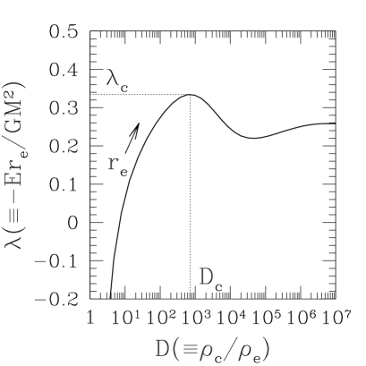
Figure 1: Energy-radius–density contrast (left) and radius-temperature–density contrast (right) relationships for the isothermal stellar system

In Fig. 1 (left), we plot the dimensionless quantity $\lambda=-r_{e}E/GM^{2}$ as a function of the density contrast $D$. Since the solid curve in this figure represents states which extremize the entropy, we note that no equilibrium state is attained when the radius of the wall $r_{e}$ is larger than the critical radius

$$r_{c}=0.335\frac{GM^{2}}{(-E)},$$ (12)

which corresponds to the state with the critical density contrast $D_{c}=709$. Furthermore, it can be shown, from a turning-point analysis for a linear series of equilibria LW1968 ; Padmanabhan1989 ; Katz1978 ; Katz1979 , that, along the curve $\lambda(D)$ derived from the condition $\delta S_{\rm BG}=0$, all states with $D>D_{c}$ are unstable. Also, the explicit evaluation of the eigenmodes for the second variation of the entropy $\delta^{2}S_{\rm BG}$ leads to the same results Padmanabhan1990 ; Padmanabhan1989 . We call this phenomenon, i.e. the absence of thermal equilibrium in self-gravitating systems when $r>r_{c}$ and/or $D>D_{c}$, the gravothermal catastrophe.

Heuristically, this instability is explained by the presence of the negative specific heat as follows. In a fully relaxed gravitating system with a sufficiently larger radius, the negative specific heat arises at the inner part of the system, where we have $C_{\rm V,inner}<0$, while the specific heat at the outer part remains positive ($C_{\rm V,outer}>0$), since one can safely neglect the effect of self-gravity. In this situation, if a tiny heat flow is momentarily supplied from the inner to the outer part, both the inner and outer parts get hotter after the readjustment of the system. Now imagine the case $C_{\rm V,outer}>|C_{\rm V,inner}|$. The outer part has so much thermal inertia that it cannot heat up as fast as the inner part, and thereby the temperature difference between inner and outer parts increases. As a consequence, the heat flow never stops, leading to a catastrophic temperature growth.

Fig. 1(right) plots the dimensionless inverse temperature $\eta\equiv GM\beta/r_{e}$ with respect to the density contrast. We can evaluate the specific heat at constant volume,

$$C_{V}\equiv\left(\frac{dE}{dT}\right)_{r_{e}}=-\beta^{2}\left(\frac{dE}{d\beta}\right)_{r_{e}}=M\eta^{2}\dfrac{\left(\dfrac{d\lambda}{dD}\right)_{r_{e}}}{\left(\dfrac{d\eta}{dD}\right)_{r_{e}}}~{}~{},$$ (13)

as shown in Fig.2.

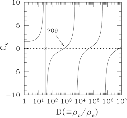
Figure 2: Specific heat as a function of the density contrast $D=\rho_{c}/\rho_{e}$ for the isotropic stellar system.

In contrast to the naive discussion for (6) based on the virial theorem, the actual specific heat (13) changes sign many times. We observe that a self-gravitating system confined by a wall of smaller radius has a positive specific heat. The reason is as follows. It can be shown that the virial theorem for a system surrounded by a boundary leads not to (4) but to

$$2K+U=3P_{e}V,$$ (14)

where $P_{e}$ is the pressure at the wall and $V$ the volume of the system (see, e.g., eq.(29) of TS2002a ). For the case of a smaller radius, the surface energy dominates the gravitational energy of the bulk so that the system behaves as a normal one; i.e. $C_{V}>0$. As the radius $r_{e}$ increases, the gravitational energy becomes significant. Eventually, the specific heat changes its sign, $C_{V}<0$ , when the value of the density contrast becomes $D=32.2$, which corresponds to a peak of the $\eta(D)$ curve (the left side of Fig.1 ).

At the onset of the gravothermal catastrophe, $D_{c}=709$, the specific heat vanishes, and $C_{V}>0$ in the unstable segment of the $\lambda(D)$ curve, $D>709$. This fact implicitly indicates a role of the negative specific heat in existence of the thermodynamic instability in self-gravitating systems. Following the previous heuristic argument, above the critical point ($D>D_{c}=709$), the specific heat of the total system becomes positive ($C_{\rm V}=C_{\rm V,inner}+C_{\rm V,outer}>0$) equivalently,

$$C_{\rm V,outer}>-\,C_{\rm V,inner}>0,$$ (15)

which means the outer normal part of the system has a larger heat capacity, so that it cannot catch up with the temperature increase of the inner part.

So far, we have discussed some interesting features of self-gravitating systems. Among these properties, the peculiarity of the system arising from the negative specific heat has been studied in terms of the Boltzmann–Gibbs entropy (7). In the next section, this sort of the analysis will be extended to that based on the non-additive entropy, i.e. the Tsallis entropy. However, before closing this section, we briefly summarize the subsequent investigation of the gravothermal catastrophe.

In this paper we adopt the thermodynamic approach in terms of the entropy and/or the free energy in order to investigate instabilities of self-gravitating systems. Although this method has the advantage of simplicity, we cannot deal with dynamical aspects of the instability appearing within the relaxation timescale (3). Typically, each particle (star) in a self-gravitating system has a long mean free path compared with its system size. In other words, during its travel across the system, the the motion of a particle is driven by the gravitational potential of the whole system and the particle experiences quite a few two-body encounters, so that the relaxation time $t_{\rm rel}$ (3) is much longer than the dynamical one $t_{\rm dyn}$ (2). This means that we cannot rely on the usual notion of local equilibrium, which is realized in cases with a short mean free path. Thus, the Fokker-Planck equation (see, e.g., chapter 8.3 of BT1987 ), which can be derived from the expansion of a collision integral in the Boltzmann equation with respect to the momentum transfer due to a two-body collision, is a useful approach for studying the long-term evolution of a self-gravitating system. By means of the linearized Fokker-Planck equation, eigenvalues and eigenfunctions which describe the time evolution of perturbations around the thermal equilibrium have been obtained Inagaki1980 .

The gas model in which a star (particle) in the self-gravitating many-body system is replaced by a gas particle, is an alternative approach. Although the gas model loses some of the basic properties of a the self-gravitating many-body system, we note that it still shows the interesting aspects of the gravothermal catastrophe. In this model, the local relaxation time is shorter than the dynamical timescale. Thus, we can introduce the usual notions of local equilibrium and the local temperature, which make our analysis much easier than in the stellar system. The local specific heat is evaluated to show that the condition (15) characterizes the onset of the gravothermal catastrophe HS1978 . The time evolution of a linear perturbation around the equilibrium gas with heat transfer has been investigated to show that the proposed mechanism for the instability based on the negative specific heat actually works in self-gravitating gaseous systems MH1991 .

3 Analysis of gravothermal catastrophe based on Tsallis’ generalized entropy

3.1 Tsallis entropy and stellar polytrope

Here we shall discuss a generalization of the analysis in previous section based on the Boltzmann–Gibbs entropy (7) to the case of the Tsallis entropy. The details are given in the literature TS2002a ; TS2002b ; TS2003 . The the energy and mass of a one- particle distribution $f(\mbox{\boldmath$x$},\mbox{\boldmath$v$})$ are respectively expressed as

$$E=K+U=\int\left\{\frac{1}{2}\,v^{2}+\frac{1}{2}\,\Phi(\mbox{\boldmath$x$})\right\}\,\,f(\mbox{\boldmath$x$},\mbox{\boldmath$v$})\,\,d^{6}\mbox{\boldmath$\tau$},$$ (16)

$$M=\int\,\,f(\mbox{\boldmath$x$},\mbox{\boldmath$v$})\,\,d^{6}\mbox{\boldmath$\tau$},$$ (17)

where the quantity $\Phi(\mbox{\boldmath$x$})$ is the gravitational potential given by

$$\Phi(\mbox{\boldmath$x$})=-G\int\frac{f(\mbox{\boldmath$x$}^{\prime},\mbox{\boldmath$v$}^{\prime})}{|\mbox{\boldmath$x$}-\mbox{\boldmath$x$}^{\prime}|}\,d^{6}\mbox{\boldmath$\tau$}^{\prime}.$$ (18)

As for generalization, the most crucial problem is the choice of the statistical average in non-extensive thermostatistics. Following a seminal paper PP1993 , the analyses in a couple of our papers TS2002a ; TS2002b have been done by utilizing the old Tsallis formalism with the standard linear mean values(see also Chavanis ; CS2003 for comparative works). On the other hand, a more sophisticated framework by means of the normalized $q$-expectation values has recently been presented TMP1998 ; MNPP2000 . As several authors have advocated, the analysis using normalized $q$-expectation values is thought to be essential, since the undesirable divergences in some physical systems can be eliminated safely when introducing the normalized $q$-expectation values. Furthermore, non-uniqueness of the Boltzmann-Gibbs theory has been shown by using normalized $q$-expectation values AR2000 . In this paper, we mainly report our investigation TS2003 based on normalized $q$-expectation values. However, this does not imply that all the analyses with standard linear means or un-normalized $q$-expectation values lose the physical significance. Actually, we observed some differences between results based on two frameworks, which will be mentioned at the end of this section.

In the new framework of Tsallis’ non-extensive thermostatistics, all the macroscopic observables of the quasi-equilibrium system can be characterized by the escort distribution, but the escort distribution itself is not thought to be fundamental. Rather, there exists a more fundamental probability function $p(\mbox{\boldmath$x$},\mbox{\boldmath$v$})$ that quantifies the phase-space structure. With the help of this function, the escort distribution is defined and the macroscopic observables are expressed as normalized $q$-expectation value as follows (see, e.g., TMP1998 ; MNPP2000 ):

escort distribution $$:P_{q}(\mbox{\boldmath$x$},\mbox{\boldmath$v$})=\frac{\displaystyle\left\{p(\mbox{\boldmath$x$},\mbox{\boldmath$v$})\right\}^{q}}{\displaystyle\int d^{6}\mbox{\boldmath$\tau$}\left\{p(\mbox{\boldmath$x$},\mbox{\boldmath$v$})\right\}^{q}}\,\,\,,$$ (19)

normalized q-value $$:\langle{\it O}_{i}\rangle_{q}=\int d^{6}\mbox{\boldmath$\tau$}\,\,{\it O}_{i}\,\,P_{q}(\mbox{\boldmath$x$},\mbox{\boldmath$v$})\,\,.$$ (20)

Based on the fundamental probability $p(\mbox{\boldmath$x$},\mbox{\boldmath$v$})$, the Tsallis entropy is given by

$$S_{q}=-\frac{1}{q-1}\,\int d^{6}\mbox{\boldmath$\tau$}\,\left[\left\{p(\mbox{\boldmath$x$},\mbox{\boldmath$v$})\right\}^{q}-p(\mbox{\boldmath$x$},\mbox{\boldmath$v$})\right].$$ (21)

Note that the probability $p(\mbox{\boldmath$x$},\mbox{\boldmath$v$})$ satisfies the normalization condition:

$$\int\,\,d^{6}\mbox{\boldmath$\tau$}\,\,p(\mbox{\boldmath$x$},\mbox{\boldmath$v$})=1.$$ (22)

To apply the above Tsallis formalism to the present problem without changing the definition of energy and mass (16) and (17), we identify the one-particle distribution with the escort distribution $P_{q}$, not the probability function $p(\mbox{\boldmath$x$},\mbox{\boldmath$v$})$:

$$f(\mbox{\boldmath$x$},\mbox{\boldmath$v$})=M\,\,\frac{\{p(\mbox{\boldmath$x$},\mbox{\boldmath$v$})\}^{q}}{N_{q}}\,\,;\,\,\,\,\,\,\,\,\,\,\,\,N_{q}=\int d^{6}\mbox{\boldmath$\tau$}\,\,\{p(\mbox{\boldmath$x$},\mbox{\boldmath$v$})\}^{q}$$ (23)

so as to satisfy mass conservation (17). The definitions of the Tsallis entropy (21) and the escort distribution (23) clearly show that the Boltzmann-Gibbs entropy (7) is recovered in the limit $q\rightarrow 1$. Now, adopting the relation (23), let us seek the extremum-entropy state under the constraints (16) and (22). The variational problem is

$$\delta\left[S_{q}-\alpha\left\{\int d^{6}\mbox{\boldmath$\tau$}p-1\right\}-\beta\left\{\int d^{6}\mbox{\boldmath$\tau$}\left(\frac{1}{2}v^{2}+\frac{1}{2}\Phi\right)f-E\right\}\right]=0,$$ (24)

where the variables $\alpha$ and $\beta$ denote the Lagrange multipliers. The variation with respect to the probability $p(\mbox{\boldmath$x$},\mbox{\boldmath$v$})$ gives the so-called stellar polytrope as the extremum-entropy state TS2003 (see also p.223 of BT1987 ):

$$f(x,v)=M\,\,\frac{\{p(x,v)\}^{q}}{N_{q}}=A\left[\Phi_{0}-\frac{1}{2}v^{2}-\Phi(x)\right]^{q/(1-q)},$$ (25)

where we define the constants $A$ and $\Phi_{0}$ as

$$A=\frac{M}{N_{q}}\,\,\left\{\frac{q(1-q)}{\alpha(1-q)+1}\frac{\beta M}{N_{q}}\right\}^{q/(1-q)},~{}~{}~{}\Phi_{0}=\frac{N_{q}}{\beta M(1-q)}+<\varepsilon>,~{}~{}~{}$$ (26)

with the quantity $<\varepsilon>$ being

$$<\varepsilon>=\frac{1}{M}\,\int d^{6}\mbox{\boldmath$\tau$}\left(\frac{1}{2}v^{2}+\Phi\right)f.$$ (27)

By means of the distribution function (25), we evaluate the density $\rho(r)$ and the isotropic pressure $P(r)$ at the radius $r=|\mbox{\boldmath$x$}|$ as

$$\rho(r) \equiv \int\frac{d^{3}\mbox{\boldmath$v$}}{h^{3}}\,\,\,f(\mbox{\boldmath$x$},\mbox{\boldmath$v$}),$$ (28)

$$= 4\sqrt{2}\pi\,B\left(\frac{3}{2},\frac{1}{1-q}\right)\,\frac{A}{h^{3}}\,\,[\Phi_{0}-\Phi(r)]^{1/(1-q)+1/2}$$

and

$$P(r) \equiv \int\frac{d^{3}\mbox{\boldmath$v$}}{h^{3}}\,\,\,\frac{1}{3}\,v^{2}\,f(\mbox{\boldmath$x$},\mbox{\boldmath$v$}),$$ (29)

$$= \frac{8\sqrt{2}\pi}{3}\,B\left(\frac{5}{2},\frac{1}{1-q}\right)\,\frac{A}{h^{3}}\,\,[\Phi_{0}-\Phi(r)]^{1/(1-q)+3/2}.$$

Here, the function $B(a,b)$ denotes the beta function. These two equations lead to the polytropic relation

$$P(r)=K_{n}\rho^{1+1/n}(r),$$ (30)

with the polytrope index $n$ related to the parameter $q$ by

$$n=\frac{1}{1-q}\,+\,\frac{1}{2}.$$ (31)

The explicit form of the dimensional constant $K_{n}$ is given in TS2003 . We note that the isothermal equation of state (11) discussed in the previous section arises in the limit $n\rightarrow\infty\,\,(q\rightarrow 1)$ as expected.

In terms of $K_{n}$ and $\rho$, the one-particle distribution can be rewritten as

$$f(x,v) = \frac{1}{4\sqrt{2}\pi\,\,B(3/2,n-1/2)}\,\,\,\frac{\rho\,\,h^{3}}{\{(n+1)\,K_{n}\,\rho^{1/n}\}^{3/2}}$$ (32)

$$~{}~{}~{}~{}~{}~{}~{}~{}~{}~{}~{}~{}~{}~{}~{}~{}~{}~{}~{}~{}~{}~{}~{}~{}~{}~{}~{}~{}~{}~{}~{}~{}\times\,\,\,\left\{1-\frac{v^{2}/2}{(n+1)\,K_{n}\,\rho^{1/n}}\right\}^{n-3/2},$$

which agrees with the result based on the old Tsallis formalism. That is to say, the equilibrium distribution (32) turns out to be invariant irrespective of the choice of the statistical averages.

We note that the equilibrium distribution (25) with (26) contains the new quantities $N_{q}$ and $<\varepsilon>$, which implicitly depend on the distribution function itself. In marked contrast to the result in the old Tsallis formalism, this fact gives rise to non-trivial thermodynamic relations as follows. By using the definitions of density and pressure (28) and (29), the quantity $<\varepsilon>$ becomes

$$<\varepsilon> = \frac{1}{M}\,\left\{\frac{3}{2}\,\int d^{3}x\,P(x)+\int d^{3}x\,\rho(x)\,\Phi(x)\,\right\}$$

$$= \frac{1}{M}\,\left\{\frac{3}{2}\,\int d^{3}x\,P(x)-\int d^{3}x\,\rho(x)\,[\Phi_{0}-\Phi(x)]\,\right\}+\Phi_{0}.$$

Furthermore, by using the relation $\Phi_{0}-\Phi(x)=(n+1)(P/\rho)$ from (28) and (29) and substituting the equation (26) into the above expression, the quantity $<\varepsilon>$ is canceled and the equation reduces to

$$\frac{N_{q}}{\beta}\,=\,\int d^{3}x\,P(x).$$ (33)

As for $N_{q}$, the normalization condition (22) gives us its actual expression TS2003 .

3.2 Gravothermal catastrophe in the stellar polytropic system

We will specifically focus on the spherically symmetric case with the polytrope index $n>3/2\,(q>0)$, in which the equilibrium distribution is at least dynamically stable (see chapter 5 of BT1987 ). In this case, the stellar equilibrium distribution can be characterized by the so-called Emden solutions (see, e.g., Chandra1939 ; KW1990 ) and all the physical quantities are expressed in terms of the homology invariant variables $(u,v)$, which are subsequently used in later analysis.

We note that the one-particle distribution function (25) does not yet completely specify the equilibrium configuration, due to the presence of the gravitational potential, which implicitly depends on the distribution function itself. Hence, we need to specify the gravitational potential or density profile. From the gravitational potential (18), we obtain the Poisson equation

$$\frac{1}{r^{2}}\frac{d}{dr}\left\{r^{2}\frac{d\Phi(r)}{dr}\right\}=4\pi G\rho(r).$$ (34)

By combining the above equation with (28), we obtain the ordinary differential equation for $\Phi$. Alternatively, a set of equations which represent the hydrostatic equilibrium are derived by using (34), (28), and (29):

$$\dfrac{dP(r)}{dr}\,= \,\,-\frac{Gm(r)}{r^{2}}\,\rho(r),$$ (35)

$$\dfrac{dm(r)}{dr}\,= \,\,4\pi\rho(r)\,r^{2}.$$ (36)

The quantity $m(r)$ denotes the mass evaluated at the radius $r$ inside the wall. Denoting the central density and pressure by $\rho_{c}$ and $P_{c}$, we then introduce the dimensionless quantities:

$$\rho=\rho_{c}\,\left[\theta(\xi)\right]^{n},\,\,\,\,\,\,r=\left\{\frac{(n+1)P_{c}}{4\pi G\rho_{c}^{2}}\right\}^{1/2}\,\xi,$$ (37)

which yields the ordinary differential equation

$$\theta^{\prime\prime}+\frac{2}{\xi}\theta^{\prime}+\theta^{n}=0,$$ (38)

where the prime denotes the derivative with respect to $\xi$. The quantities $\rho_{c}$ and $P_{c}$ in (37) are the density and the pressure at $r=0$, respectively. To obtain the physically relevant solution of (38), we use the boundary condition

$$\theta(0)=1,\,\,\,\,\,\,\,\theta^{\prime}(0)=0.$$ (39)

A family of solutions satisfying (39) is referred to as the Emden solution, which is well-known in the subject of stellar structure (see, e.g., chapter IV of ref.Chandra1939 ). To characterize the equilibrium properties of Emden solutions, it is convenient to introduce the following set of variables, referred to as homology invariants Chandra1939 ; KW1990 :

$$u \equiv \frac{d\ln m(r)}{d\ln r}=\frac{4\pi r^{3}\rho(r)}{m(r)}=-\frac{\xi\theta^{n}}{\theta^{\prime}},$$ (40)

$$v \equiv -\frac{d\ln P(r)}{d\ln r}=\frac{\rho(r)}{P(r)}\,\,\frac{Gm(r)}{r}=-(n+1)\frac{\xi\theta^{\prime}}{\theta},$$ (41)

which reduce the degree of (38) from two to one. Recall that we are investigating the thermodynamic properties of a self-gravitating system within a wall of radius $r_{e}$. We can evaluate the total energy of the confined stellar system in terms of the pressure $P_{e}$, the density $\rho_{e}$ at the boundary $r_{e}$, and the total mass $M$:

$$E=K+U = \frac{3}{2}\,\int_{0}^{r_{e}}dr\,4\pi r^{2}\,P(r)-\int_{0}^{r_{e}}\,dt\,\frac{Gm(r)}{r}\,\frac{dm}{dr}$$

$$= -\frac{1}{n-5}\,\left[\,\frac{3}{2}\left\{\frac{GM^{2}}{r_{e}}-(n+1)\frac{MP_{e}}{\rho_{e}}\right\}+(n-2)\,4\pi\,r_{e}^{3}\,P_{e}\,\right],$$

by which the dimensionless quantity $\lambda$ can be expressed as a function of the homology invariants at the wall TS2002a ; TS2002b ; TS2003 :

$$\lambda\equiv-\dfrac{Er_{e}}{GM^{2}}=-\frac{1}{n-5}\,\left[\,\frac{3}{2}\left\{1-\frac{n+1}{v_{e}}\right\}+(n-2)\frac{u_{e}}{v_{e}}\,\right].$$ (42)

Figure 3: Energy-radius-density contrast relationship for the stellar polytropes with various indices.

As was already shown in section 2 for the isothermal case, the above dimensionless quantity $\lambda$ has an important role for the analysis of the gravothermal catastrophe. Figure 3 shows $\lambda$ as a function of the ratio of the central density to that at the boundary, $\rho_{c}/\rho_{e}$. We notice that the $\lambda$-curves are bounded from above and have peaks in the case of $n>5$ (right panel). On the other hand, the curves for $n\leq 5$ monotonically increase (left panel). It follows that the stellar polytrope within an adiabatic wall exhibits the gravothermal instability in the case of a polytropic index $n>5$. Similarly to the isothermal case, the evaluation of eigenvalues for the second variation of the Tsallis entropy $\delta^{2}S_{q}$ gives the same results as the above turning point analysis in terms of the $\lambda$-curve TS2002a ; TS2002b ; TS2003 .

3.3 Thermodynamic instability arising from the negative specific heat

As discussed in the isothermal case in the previous section, thermodynamic instability in stellar systems is intimately related to the presence of a negative specific heat LW1968 ; LyndenBell1999 . The evaluation of the specific heat is thus necessary for clarifying the thermodynamic properties. In this regard, the identification of the temperature in the stellar system in the polytropic case is the most essential task.

In the new framework of Tsallis’ non-extensive thermostatistics, the physically plausible thermodynamic temperature $T_{\rm phys}$ can be defined from the zero-th law of thermodynamics AMPP2001 ; Abe2001 ; MPP2001 . The thermodynamic temperature in a non-extensive system differs from the usual one, i.e., the inverse of the Lagrange multiplier $\beta$. The pseudo-additivity of the Tsallis entropy and the transitivity of thermal equilibria suggests

$$T_{\rm phys}=\,[1+(1-q)\,S_{q}]\,\,\beta^{-1}.$$ (43)

Here, the relation (43) should be carefully applied to the present case, since the verification of zero-th thermodynamic law is very difficult in a stellar equilibrium system with long-range interactions. Furthermore, even using the new formalism, the energy $E$ remains non-extensive due to the self-referential form of the potential energy (see (16) and (18)). However, the consistency of the physical temperature given by (43) can be shown by an alternative argument TS2002b ; TS2003 for the self-gravitating stellar system, where the modified Clausius relation AMPP2001 ; Abe2001 ; MPP2001

$$dS_{q}=\frac{1}{T_{\rm phys}}\{1+(1-q)\,S_{q}\}\,d^{\prime}Q.$$

plays a significant role.

From the expression for the normalization factor $N_{q}$ of the escort distribution (23), the Tsallis entropy (21) of the extremum state is given by

$$S_{q}=\dfrac{1}{1-q}\,\,(N_{q}-1).$$

Let us substitute this expression into (43). Then, the relation (33) for $N_{q}/\beta$ gives us the expression of the thermodynamic temperature $T_{\rm phys}$ as an integral of a physical quantity, i.e. the pressure distribution:

$$T_{\rm phys}=\dfrac{N_{q}}{\beta}=\int d^{3}x\,P(x).$$ (44)

We can evaluate the above integral to represent the thermodynamic temperature in terms of the pressure $P_{e}$, the density $\rho_{e}$ at the boundary and the total mass $M$ as

$$T_{\rm phys}=-\frac{1}{n-5}\left\{8\pi\,r_{e}^{3}P_{e}-(n+1)\frac{MP_{e}}{\rho_{e}}+\frac{GM^{2}}{r_{e}}\right\}$$ (45)

from which the dimensionless inverse temperature is denoted by

$$\eta\equiv\frac{GM^{2}}{r_{e}T_{\rm phys}}=\frac{(n-5)\,v_{e}}{n+1-2u_{e}-v_{e}}$$ (46)

as a function of the homology invariant at the boundary TS2003 . From (42) and (46), the specific heat at constant volume $C_{\rm\scriptscriptstyle V}$ is given by

$$C_{\rm\scriptscriptstyle V}\equiv\left(\frac{d\,E~{}~{}~{}}{d\,T_{\rm phys}}\right)_{e}=\eta^{2}\frac{\displaystyle\left(\frac{d\lambda}{d\xi}\right)_{e}}{\displaystyle\left(\frac{d\eta}{d\xi}\right)_{e}}.$$ (47)

Figure 4: Specific heat as a function of the density contrast for the stellar polytropes with $n=3$ (left) and $n=6$ (right).

In order to compare with the behavior of the specific heat in the isothermal case of Fig. 2, we plot $C_{\rm\scriptscriptstyle V}$ with respect to the density contrast for several values of the polytropic index in Fig. 3.2.

As already denoted at the end of subsection 3.2, the stellar polytropic system exhibits the gravothermal catastrophe when the polytropic index $n$ is larger than the critical value, i.e. $n>5$. In the isothermal case, the onset of the thermodynamic instability is characterized by the condition (15). Figure 4 shows that the thermodynamic argument based on the negative specific heat for the gravothermal catastrophe can be extended to the case of the stellar polytrope, i.e. the equilibrium of the self-gravitating system described by the extremum of the Tsallis entropy.

Figure 5: Density profiles of the stellar polytropes for $n<5$ (left) and $n\geq 5$ (right).

In Fig. 5, we depict the density profiles with respect to the dimensionless radius $\xi$ (37). Clearly, profiles with index $n<5$ rapidly fall off and they abruptly terminate at finite radius(left panel), while the $n\geq 5$ cases infinitely continue to extend over the outer radius(right panel). It follows that stellar polytropic systems with index $n\geq 5$ are able to possess a sufficient amount of the outer normal part to realize the gravothermal catastrophe.

Before closing this section, we mention differences between the old and new Tsallis formalisms. First, the relationship between the polytrope index $n$ and theTsallis parameter $q$ in (31) differs from the one obtained previously, but is related to it through the duality transformation, $q\leftrightarrow 1/q$ (see (14) in TS2002a or (12) in TS2002b ). This property was first addressed in TMP1998 in a more general context, together with changes to the Lagrangian multiplier $\beta$. The duality relation implies that all of the thermodynamic properties in the new formalism can also be translated into those obtained in the old formalism. Secondly , in previous studies TS2002b based on the standard linear means, the radius-mass-temperature relation and the specific heat seriously depend on the dimensional parameter for the phase element $h$ (8). By contrast, in the present case TS2003 , the radius-mass-temperature relation was derived from the non-trivial relation (33), in which no such $h$-dependence appears. The resultant specific heat is also free from this dependence, which is a natural outcome of the new framework using the normalized $q$-expectation values. Therefore, it seems likely that the new formalism provides a better characterization for non-extensive quasi-equilibrium systems.

4 Reality of the stellar polytrope as a quasi-equilibrium state

So far, we have discussed the extension of the thermodynamic analysis to the stellar polytrope which is obtained by applying the variational procedure to the Tsallis entropy for the stellar self-gravitating system. It has been shown that thermodynamic quantities such as the specific heat are useful for studying the emergence of the gravothermal catastrophe in the stellar polytrope. In Fig. 6 we summarize our results. The stellar polytrope confined by an adiabatic wall is shown to be thermodynamically stable when the polytrope index $n<5$. In other words, if $n>5$, a stable equilibrium state ceases to exist for a sufficiently large density contrast $D>D_{\rm crit}$, where the critical value $D_{\rm crit}$ given by a function of $n$ is determined from the second variation of the entropy around the extremum state of the Tsallis entropy, $\delta^{2}S_{q}=0$TS2002a ; TS2003 . The dotted line in Fig.6 represents the critical value $D_{\rm crit}$ for each polytrope index, which indicates that the stellar polytrope at low density contrast $D<D_{\rm crit}$ is expected to remain stable.

The above arguments indicate that, similar to the isothermal state, the stellar polytropic distribution can also be regarded as an equilibrium state, since it is described by the extremal state of the Tsallis entropy. However, the one-particle distribution function of the stellar polytrope (32) clearly shows that the velocity dispersion,

$$\sigma(r)\propto\frac{1}{\rho(r)}\,\,\int\frac{d^{3}\mbox{\boldmath$v$}}{h^{3}}\,\,\,v^{2}\,f(\mbox{\boldmath$x$},\mbox{\boldmath$v$}),$$ (48)

depends on the radius $r$. Only in the isothermal case, $n\rightarrow\infty$, is $\sigma$ spatially constant. Thus, it is expected that a gradient of the velocity dispersion is relaxed within the time scale due to two-body collisions (3). This means that the stellar polytrope is no longer the equilibrium but a quasi-equilibrium state. In this section, we report the results of $N$-body simulations TSPRL which were carried out to investigate how the stellar polytrope actually evolves.

The $N$-body experiment considered here is the same as that investigated in classic papers (Antonov1962 ; LW1968 ; see also EFM1997 ). That is, we confine the $N$ particles interacting via Newtonian gravity in a spherical adiabatic wall, which reverses the radial components of the velocity if the particles reach the wall. Without loss of generality, we set the units as $G=M=r_{e}=1$. Note that the typical time scales appearing in this system are the dynamical time $t_{\rm dyn}$ (2) and the global relaxation time driven by the two-body encounter, $t_{\rm rel}$ (3), which are basically scaled as $t_{\rm dyn}\sim 1$ and $t_{\rm rel}\sim 0.1N/\ln N$ in our units.

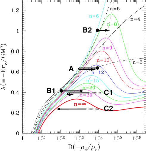
Figure 6: Equilibrium sequences of the stellar polytrope and the isothermal distribution ($n=\infty$) in the $\lambda\equiv-r_{e}E/(GM^{2})$ vs $D\equiv\rho_{c}/\rho_{e}$ plane. The thick arrows denote the evolutionary tracks in each simulation run (see Sec.4).

Table 1: Initial distributions and their evolutionary states

run no.	initial distribution	parameters	no. of particles	transient state	final state
A	stellar polytrope($n=3$)	$D=10,000$	2,048	stellar polytrope	collapse
B1	stellar polytrope($n=6$)	$D=110$	2,048	stellar polytrope	collapse
B2	stellar polytrope($n=6$)	$D=10,000$	2,048	stellar polytrope	collapse
C1	Hernquist model	$a/r_{e}=0.5$	8,192	stellar polytrope	collapse
C2	Hernquist model	$a/r_{e}=1.0$	8,192	none	isothermal

Table 1 summarizes the five simulation runs. Here, in addition to the stellar polytropic initial state, we also consider the non-stellar polytropic state of the Hernquist model H1990 , which was originally introduced to account for the empirical law of observed elliptical galaxiesBT1987 .

As was expected, the numerical simulations reveal that the stellar polytropic distribution gradually changes with time, on the time scale of two-body relaxation (3). Furthermore, focusing on the evolutionary sequence, we found that the transient state starting from the initial stellar polytrope can be remarkably characterized by a sequence of stellar polytropes (run A, B1, and B2). This is even true in the case starting from the Hernquist model (run C1).

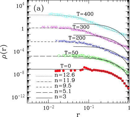
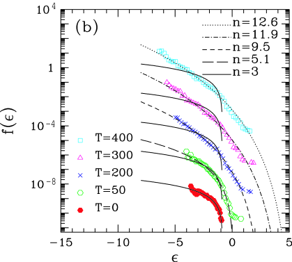
Figure 7: Results from simulation run A: (a) snapshots of the density profile $\rho(r)$, and (b) snapshots of the one-particle distribution function $f(\epsilon)$.

Let us show representative results taken from run A (Fig.7). Figure 7(a) plots snapshots of the density profile $\rho(r)$, while Fig.7(b) represents the distribution function $f(\varepsilon)$ as a function of the specific energy $\varepsilon=\frac{1}{2}v^{2}+\Phi(\mbox{\boldmath$x$})$. Note, for illustrative purpose, that each output result is artificially shifted to the two digits below. Only the final output with $T=400$ represents the correct scales. In each figure, solid lines mean the initial stellar polytrope with $n=3$ and the other lines indicate the fitting results to the stellar polytrope by varying the polytrope index $n$. Note that the number of fitting parameters just dexreases to one, i.e. the polytrope index, since the total energy is well-conserved in the present situation. Fig.7 shows that while the system gradually deviates from the initial polytropic state, the transient state still follows a sequence of stellar polytropes. The fitting results are remarkably good until the time exceeds $T\simeq 400$, corresponding to $15\,t_{\rm rel}$. After that, the system enters the gravothermally unstable regime and finally undergoes the core collapse.

Now, focus on the evolutionary track in each simulation run summarized in the energy-radius-density contrast plane (Fig.6), where the filled circle represents the initial stellar polytrope. Interestingly, the density contrast of the transient state in run A initially decreases, but it eventually turns to increase. The turning point roughly corresponds to the stellar polytrope with index $n\sim 5-6$. Note, however, that the time evolution of the polytrope index itself is a monotonically increasing function of time TSPRL . This is indeed true for the other cases, indicating the Boltzmann $H$-theorem that any self-gravitating system tends to approach the isothermal state. A typical example is run C2, which finally reaches the stable isothermal state. However, as already shown in run A, not all the systems can reach the isothermal state. Fig.6 indicates that no isothermal state is possible for a fixed value $\lambda>0.335$Antonov1962 ; LW1968 , which can be derived from the peak value of the trajectory. Further, stable stellar polytropes cease to exist at a high density contrast, $D>D_{\rm crit}$. In fact, our simulations starting from the stellar polytropes finally underwent core collapse due to the gravothermal catastrophe (runs A, B1, and B2). Though it might not be rigorously correct, the predicted value $D_{\rm crit}$ provides a crude approximation to the boundary between stability and instability.

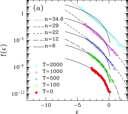
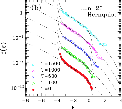
Figure 8: Evolution of the one-particle distribution function in other models: (a) run B1; (b) run C1

Fig.8 plots snapshots of the distribution function taken from the other runs. The initial density contrast in run B1 (Fig.8(a)) is relatively low ($D=110$) and therefore the system slowly evolves by following a sequence of stellar polytropes. After $T=2000\sim 74\,\,t_{\rm rel}$, the system begins to deviate from the stable equilibrium sequence, leading to core collapse. Another noticeable case is run C1 (Fig.8(b)). The Hernquist model as the initial distribution of run C has a cuspy density profile, $\rho(r)\propto 1/r/(r+a)^{3}$, which behaves as $\rho\propto r^{-1}$ at the inner part H1990 . The resultant distribution function $f(\varepsilon)$ shows singular behavior at the negative energy region, which cannot be described by the power-law distribution. Soon after, however, gravothermal expansionEFM1997 takes place and a flatter core is eventually formed. Then the system settles into a sequence of stellar polytropes and can be approximately described by the stellar polytrope with index $n=20$ for a long time. Thus the stellar polytrope can be regarded as a quasi-attractor and a quasi-equilibrium state.

5 Conclusion and Discussion

In this paper, we discussed issues arising from the Tsallis entropy for the thermodynamic properties of stellar self-gravitating systems, with a particular emphasis on the standard framework using normalized $q$-expectation values. It turns out that the new extremum-entropy state essentially remains unchanged from previous studies and is characterized by the stellar polytrope, although the distribution function shows several distinct properties. By considering these facts carefully, the thermodynamic temperature of the extremum state was identified through the modified Clausius relation and the specific heat was evaluated explicitly. A detailed analysis of the behavior of specific heat finally led to the conclusion that the onset of gravothermal instability remains unchanged with respect to choice of the statistical average for a system confined by an adiabatic wall (micro-canonical case). As for a system surrounded by a thermal wall (canonical case), although the analysis has been skipped in this article, the stability of the system drastically depends on the choice of the statistical average TS2002b ; TS2003 . The existence of these thermodynamic instabilities can also be deduced rigorously from the variation of the entropy and free energy TS2002a ; TS2002b ; TS2003 . As a result, above certain critical values of $\lambda$ or $D$, the thermodynamic instability appears at $n>5$ for a system confined by an adiabatic wall.

We performed a set of numerical simulations of long-term stellar dynamical evolution away from the isothermal state and found that the transient state of a system confined by an adiabatic wall can be remarkably fitted by a sequence of stellar polytropes. This is even true for the case in which the outer boundary in removed TSPRL . Therefore, the stellar polytropic distribution can be a quasi-attractor and a quasi-equilibrium state of a self-gravitating system.

Appendix A Appendix:  Evaluation of the relaxation time

Here we briefly evaluate the relaxation time for a self-gravitating many-body system (3). For a more precise derivation, consult BT1987 ; Chandra . In the kinetic theory, a time scale of relaxation due to two-body collisions is given by

$$t_{\rm rel}\sim\dfrac{1}{\sigma nv},$$ (49)

where $n$ is the mean number density and $v$ the average relative velocity of particles. In order to evaluate theamplitude of a two-body collision by the mutual gravitational force, we introduce the gravitational radius $r_{\rm g}$ as follows,

$$mv^{2}\sim\frac{Gm^{2}}{r_{\rm g}}~{}~{}~{}~{}\longrightarrow~{}~{}~{}~{}r_{\rm g}\sim\frac{Gm}{v^{2}}.$$ (50)

If the impact parameter of the collision between two particles of identical mass $m$ becomes smaller than the gravitational radius, i.e. $b<r_{\rm g}$, orbits of particles are significantly changed by the close encounter. It follows that the cross section of a two-body collision is given by

$$\sigma\sim 4\pi r_{g}^{2}.$$ (51)

By substituting this estimate and $n\sim N/R^{3}$ into (49), we obtain

$$t_{\rm rel}\sim\frac{v^{3}R^{3}}{4\pi\,G^{2}\,m^{2}\,N\,\ln\left(R/r_{g}\right)},$$ (52)

where $R$ and $N$ are the system size and the number of particles, respectively. In the above expression (52), we have included the so–called Coulomb logarithm term, $\ln(R/r_{g})$, which appears due to the long-range nature of the interaction BT1987 and is well-known in plasma theory. By taking its ratio to the dynamical time $t_{\rm dyn}\sim R/v$, we obtain

$${t_{\rm rel}}\sim\frac{N}{4\pi\ln N}\,{t_{\rm dyn}}\,,$$ (53)

where the average velocity is estimated as $v^{2}\sim{GNm}/{R}$ from the virial theorem (4).

References

- (1) J. Binney, S. Tremaine, Galactic Dynamics (Princeton Univ. Press, Princeton, 1987)
- (2) L. Spitzer, Dynamical Evolution of Globular Clusters, (Princeton Univ. Press, Princeton, 1987).
- (3) R. Elson, P. Hut, S. Inagaki, Ann. Rev. Astron. Astrophys. 25 (1987) 565.
- (4) G. Meylan, D.C. Heggie, Astron.Astrophys.Rev. 8 (1997) 1.
- (5) V.A. Antonov, Vest. Leningrad Gros. Univ., 7 (1962) 135 (English transl. in IAU Symposium 113, Dynamics of Globular Clusters, ed. J. Goodman and P. Hut [Dordrecht: Reidel], pp. 525–540 [1985])
- (6) D. Lynden-Bell, R. Wood, Mon.Not.R.Astr.Soc. 138 (1968) 495.
- (7) T. Padmanabhan, Phys.Rep. 188 (1990) 285.
- (8) C. Tsallis, J.Stat.Phys. 52 (1988) 479.
- (9) S. Abe, Y. Okamoto (Eds.), Nonextensive Statistical Mechanics and Its Applications (Springer, Berlin, 2001)
- (10) G. Kaniadakis, M. Lissia, A. Rapisarda (Eds), Non-Extensive Thermodynamics and Physical Applications special issue, Physica A 305 (2002)
- (11) A.R. Plastino, A. Plastino, Phys.Lett. A 174 (1993) 384.
- (12) J.-J. Aly, in N-body Problems and Gravitational Dynamics, Proceedings of a meeting held at Aussois-France (21-25 March 1993), (eds.) F. Combes, E. Athanassoula (Publications de l’observatiore de Paris, Paris, 1993), p.19.
- (13) J.A.S. Lima, R. Silva, J. Santos, Astron. Astrophys. 396 (2002) 309.
- (14) A. Taruya, M. Sakagami, Physica A 307 (2002) 185.
- (15) A. Taruya, M. Sakagami, Physica A 318 (2003) 387.
- (16) A. Taruya, M. Sakagami, Physica A 322 (2003) 285.
- (17) A. Taruya, M. Sakagami, Phys. Rev. Lett.90 (2003) 181101.
- (18) S. Chandrasekhar, Principles of Stellar Dynamics (Univ. of Chicago Press, 1942)
- (19) T. Padmanabhan, Astrophys.J.Suppl. 71 (1989) 651.
- (20) J. Katz, Mon.Not.R.Astr.Soc. 183 (1978) 765.
- (21) J. Katz, Mon.Not.R.Astr.Soc. 189 (1979) 817.
- (22) Publ. Astron. Soc. Japan 32 (1980) 213.
- (23) I. Hachisu, D. Sugimoto, Prog. Theor. Phys. 60 (1978) 393.
- (24) J. Makino, P. Hut, Astrophys.J. 383 (1991) 181.
- (25) P.H. Chavanis, Astron.Astrophys. 386 (2002) 732; ibid. 401 (2003) 15.
- (26) P.H. Chavanis, C. Sire, Phys.Rev.E, in press (cond-mat/0303088).
- (27) C. Tsallis, R.S. Mendes, A. R. Plastino, Physica A 261 (1998) 534.
- (28) S. Martínez, F. Nicolás, F. Pennini, A. Plastino, Physica A 286 (2000) 489.
- (29) S. Abe, A. K. Rajagopal, Phys.Lett. A 272 (2000) 345; J. Phys. A 33 (2000) 8733; Europhys. Lett. 52 (2000) 610.
- (30) S. Chandrasekhar, Introduction to the Study of Stellar Structure (New York, Dover, 1939)
- (31) R. Kippenhahn, A. Weigert, Stellar Structure and Evolution (Springer, Berlin, 1990)
- (32) D. Lynden-Bell, Physica A 263 (1999) 293.
- (33) S. Abe, S. Martínez, F. Pennini, A. Plastino, Phys.Lett. A 281 (2001) 126.
- (34) S. Abe, Physica A 300 (2001) 417.
- (35) S. Martínez, F. Pennini, A. Plastino, Physica A 295 (2001) 416.
- (36) H. Endoh, T. Fukushige, J. Makino, Publ. Astron. Soc. Japan 49 (1997) 345.
- (37) L. Hernquist, Astrophys. J. 356 (1990) 359.