Effects of electrostatic fields and Casimir force
on cantilever vibrations

Abstract

The effect of an external bias voltage and fluctuating electromagnetic fields on both the fundamental frequency and damping of cantilever vibrations is considered. An external voltage induces surface charges causing cantilever-sample electrostatic attraction. A similar effect arises from charged defects in dielectrics that cause spatial fluctuations of electrostatic fields. The cantilever motion results in charge displacements giving rise to Joule losses and damping. It is shown that the dissipation increases with decreasing conductivity and thickness of the substrate, a result that is potentially useful for sample diagnostics. Fluctuating electromagnetic fields between the two surfaces also induce attractive (Casimir) forces. It is shown that the shift in the cantilever fundamental frequency due to the Casimir force is close to the shift observed in recent experiments of Stipe et al. [1]. Both the electrostatic and Casimir forces have a strong effect on the cantilever eigenfrequencies, and both effects depend on the geometry of the cantilever tip. We consider cylindrical, spherical, and ellipsoidal tips moving parallel to a flat sample surface. The dependence of the cantilever effective mass and vibrational frequencies on the geometry of the tip is studied both numerically and analytically.

I Introduction

The description of the motion of a microscopically small body near a massive solid is an important problem in various areas of modern physics, including atomic, scanning tunneling, and magnetic resonance force microscopies. The interactions between bodies separated by a vacuum arise from electromagnetic fields of various types, the simplest example being an external potential difference applied between metallic bodies. In this case the surfaces in close proximity acquire opposite electric charges and experience an electrostatic attraction. A static electric field between different surfaces may exist even without any externally applied voltage; a zero-bias electrostatic attraction may be caused by local variations in the work function or surface contamination resulting in an inhomogeneous electric field. This is referred to as the patch effect (see, for instance, References [2]-[4]). Also, spatial fluctuations of the electric field may be caused by charged defects in the bulk of a cantilever or a sample. In addition to these electrostatic effects, electrically neutral bodies interact via fluctuating electromagnetic fields. Fluctuating electric currents and charge densities (or polarizations) of a given body produce fields that act on other bodies. The strength of the interaction depends on the power spectrum of the fluctuations, which in turn are determined by the complex dielectric permittivity. Lifshitz treated this van der Waals force in a classic paper [5]. In the case of high-conductivity metal surfaces the effect is referred to as the Casimir force, which has been the subject of several recent experiments [6]-[9] and various surveys (see, for instance, Reference [10] and monographs [11],[12]).

When a vibrating cantilever approaches a sample there is an increase in the dissipative force it experiences. Because of its great practical importance, the problem of noncontact friction has become a topic of increasing interest (see, for instance, References [13]-[20]). The utilization of micromechanical cantilevers could conceivably be extended considerably if the physical mechanisms responsible for the damping were understood. Such an understanding might lead to applications in which both the conservative (elastic or electrostatic) forces and the dissipative (velocity-dependent) forces are probed in order to obtain useful information about a sample.

Attempts to explain the observed friction in terms of the van der Waals interaction [18],[21]-[23] have not met with much success [15],[19],[20]. On the other hand the effect of electric fields of various origins on the noncontact friction was shown in the experiments of Stipe et al. [1] to play an important role in determining the friction, although a microscopic theory still does not exist. It follows from the work of Stipe et al. [1] that any changes in the electric field (due, for example, to changes of tip-surface distance or variations in bias voltage associated with charge defects generated in dielectric substrates) produce significant modifications of the noncontact friction.

In what follows we consider the perpendicularly oriented cantilever, which has been utilized as an ultrasensitive device for the study of forces and dissipation at small length scales [1]. The perpendicular orientation allows a much closer approach of the tip to the sample without jump-to-contact, and also much less cantilever damping than in the parallel configuration. The influence of tip-substrate attraction on cantilever eigenfrequencies and Joule dissipation will be studied, and the dependence of these quantities on the tip geometry will be described both analytically and numerically.

In Section II we develop expressions for the electric field , induced currents, and Joule heating in the case of a cylindrical tip. We consider both infinitely thick and finite-thickness substrates, and find that Joule heating is increased in the case of a thin substrate. Section III extends this analysis to the more realistic case of spherical or ellipsoidal tips, and in Section IV we consider the Casimir force, which can be the dominant force at small tip-sample separations, for both cylindrical and ellipsoidal tips. In Section V we consider the force arising from spatial fluctuations of electrostatic charge, and compare this force to the Casimir force for typical parameters of interest. Section VI is concerned with the effects of these attractive forces on the vibrational frequency and effective mass of the cantilever, and numerical results for these effects are given for typical values of various parameters. Our conclusions are summarized in Section VII.

II Electric field and induced currents for a cylindrical tip geometry

In this section we consider first a model in which the cantilever tip is assumed to be a metallic cylinder with its axis parallel to a flat sample surface. The tip displacements are assumed to be nearly parallel to the surface, which will be the case when the oscillation amplitudes are sufficiently small. Figure 1 shows the model under consideration. The cantilever width $b$ is taken to be much larger than the thickness $a$ ($b\gg a$). Figure 1 shows a section in the plane of the cantilever motion. It is straightforward to obtain the static electric field distribution in the practically important case of small distances $d$ such that the electrostatic field of the entire cylinder is effectively the same as that due only to its bottom part. (The criterion that $d$ must satisfy for this to be the case is given below.) The problem is then reduced to solving the 2D Laplace equation with the boundary conditions that the potential has constant values $\phi_{1}$ and $\phi_{2}$ at the metallic surfaces. The electric field distribution outside the conductors is equal to the field due to a charge $q$ and its image $-q$ placed at a distance $d_{1}=[(R+d)^{2}-R^{2}]^{1/2}$ from the surface. (Details may be found in Reference [24].) $q$ represents charge per unit length along the $y$ direction, and is determined by the potential difference $\phi_{1}-\phi_{2}$ and the capacitance $C$ given by

$$C^{-1}=2{\rm cosh}^{-1}(1+d/R)=2\ln\left[(d+R+d_{1})/R\right]\ .$$ (1)

Thus [24]

$$q=C(\phi_{1}-\phi_{2})\ .$$ (2)

The electric field at a point ${\bf r}$ exterior to the tip and sample is given by

$${\bf E}({\bf r})=2q\left[{{\bf r}-{\bf r}_{1}\over|{\bf r}-{\bf r}_{1}|^{2}}-{{\bf r}-{\bf r}_{2}\over|{\bf r}-{\bf r}_{2}|^{2}}\right]\ ,$$ (3)

where ${\bf r}_{1}$ and ${\bf r}_{2}$ denote the positions of $+q$ and -$q$, respectively. For the coordinate system shown in Figure 1, ${\bf r}_{1,2}=\pm d_{1}{\bf e}_{z}$, where ${\bf e}_{z}$ is the unit vector along the $z$ axis. The attractive cantilever-surface force can be calculated straightforwardly using Eqs. (1)-(3). We obtain

$$T=bq^{2}/d_{1}$$ (4)

for the force on the tip. $T$ is proportional to the length $b$ of the cylindrical tip in our model, and is given by

$$T={bV^{2}R^{1/2}\over 2^{7/2}d^{3/2}}\ ,\ \ \ \ V=\phi_{1}-\phi_{2}$$ (5)

in the practically important case $d\ll R$.

Metals are almost inpenetrable by the electric field, the penetration being restricted to a very thin surface layer (Debye layer) of thickness $R_{D}$ considerably less than other characteristic lengths of the system, i.e., $R_{D}\ll R,d,d_{1}$. Integrating the Poisson equation over a thin layer of the sample (but with thickness greater than $R_{D}$), we obtain the surface charge density

$$\sigma(x)=-{qd_{1}\over\pi[x^{2}+d_{1}^{2}]}\ ,$$ (6)

where we have taken into account the boundary conditions $E_{z}(z=0^{+})=-4qd_{1}/(x^{2}+d_{1}^{2})$ and $E_{z}(z=0^{-})=0$. The last condition, of course, means that the overall field due to the charged tip and the surface (Debye) layer is zero in the volume of the metal substrate.

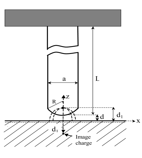
FIG. 1.: Cantilever-sample geometry for the model in which the cantilever “tip” is taken to be part of a cylinder of radius $R$.

A somewhat different picture applies in the case of a moving charged tip. To be specific, we consider the case of oscillatory motion of the tip: $X(t)=X_{0}\cos\omega t$. (Note that an oscillating cantilever is used, for example, for spin detection [25].) The cantilever charge is not changed when its tip moves parallel to the surface, while the sample charge varies in time at any fixed point. The varying sample charge induces an electric current, and the charge and current are related by the continuity equation, $\partial\rho/\partial t+\nabla\cdot{\bf J}=0$, where $\rho$ and ${\bf J}$ are the charge and current densities, respectively. Integration of the continuity equation over a small element of surface layer gives the relation between the normal current near the Debye layer and the time derivative of the surface charge density:

$${\partial\over\partial t}\sigma(x,t)=J_{z}(x,z=0^{-},t)\ .$$ (7)

We will assume that the cantilever motion is slow in the sense that $\omega\ll 4\pi\mu$, where $\mu$ is the sample conductivity; in this case an iterative procedure described by Boyer [26] is applicable. The assumption of slow cantilever motion means that the surface charge follows the tip displacements practically instantaneously. To lowest order in the parameter $\omega/(4\pi\mu)$, the surface charge may be approximated by Eq. (6) with the coordinate $x$ replaced by $x-X(t)$. This approximation corresponds to an effectively infinite value of volume conductivity and instantaneous recharging. Then, from Eq. (7),

$$J_{z}(x,z=0^{-},t)=\mu E_{z}(x,z=0^{-},t)=-{1\over\pi}qd_{1}\omega X_{0}\sin\omega t{\partial\over\partial x}{1\over(x-X)^{2}+d_{1}^{2}}\ .$$ (8)

The additional surface charge $\sigma^{\prime}$ (up to first order in $\omega/mu$) caused by the normal current (8) can easily be obtained by considering this charge as a source of the field $E_{z}(x,z=0^{-},t)$. Taking into account the fact that the field $E_{z}$ induced by the additional surface charge has opposite signs below and above the surface $z=0$, we obtain the perturbation of the surface charge density as follows:

$$\sigma^{\prime}(x,t)={qd_{1}\omega X_{0}\sin\omega t\over 2\pi^{2}\mu}{\partial\over\partial x}{1\over(x-X)^{2}+d_{1}^{2}}\ .$$ (9)

For small tip oscillation amplitudes $(X_{0}\ll d_{1})$ we can ignore $X(t)$ in the denominator. Thus we obtain the electric field due to the surface charge $\sigma^{\prime}$:

$${\bf E}^{\prime}({\bf r},t)=2\int_{-\infty}^{\infty}dx^{\prime}\sigma^{\prime}(x^{\prime},t){\partial\over\partial{\bf r}}\ln|{\bf r}-{\bf e}_{x}x^{\prime}|\ .$$ (10)

Explicitly, the expression for the electric field that is first-order in $\omega/\mu$ is

$${\bf E}^{\prime}({\bf r},t)={q\omega X_{0}\sin\omega t\over\pi\mu}{\partial\over\partial d_{1}}\left({-{\bf e}_{x}(|z|+d_{1})\pm{\bf e}_{z}x\over x^{2}+(|z|+d_{1})^{2}}\right)\ ,$$ (11)

where the $+$ and - signs correspond to $z>0$ and $z<0$, respectively. It follows from Eq. (11) that the characteristic length of the electric field variation is $d_{1}$. Hence our simplifying assumption that the field formed by the full cylinder can be represented by only its bottom part (as in Figure 1) is valid in the case $d_{1}\ll R$.

Equation (11) can be used to obtain the cantilever damping due to Joule dissipation. The Joule power $W_{j}$ is given by the integral

$$W_{j}={b\mu}\int_{-\infty}^{\infty}dx\int_{-\infty}^{0}dz\left[{\bf E}^{\prime}({\bf r},t)\right]^{2}\ ,$$ (12)

which, when used with Eq. (11), becomes

$$W_{j}={b(qX_{0}\omega)^{2}\over 8\pi\mu d_{1}^{2}}\approx{b(VX_{0}\omega)^{2}\over 2^{7}\pi\mu d^{2}}\ .$$ (13)

Note that there is no dependence of $W_{j}$ on the tip radius $R$. This results from the effects of two competitive factors determining the Joule loss. The first is the magnitude of the electric field in the bulk of the substrate, which increases with a decrease in the characteristic inhomogeneity size $d_{1}\approx(2dR)^{1/2}$ as $R/d_{1}^{3}$. The second is the characteristic volume $\sim d_{1}^{2}$ contributing to the integral in Eq. (12). Thus the two effects together vary as $(R/d_{1}^{3})^{2}d_{1}^{2}\propto 1/d^{2}$, and have no net dependence on $R$.

The damping of the cantilever oscillations can be described alternatively as follows. It can be seen from Eq. (11) that there exists not only a $z$-component, but also an $x$-component of the field ${\bf E}^{\prime}$, i.e., a component parallel to the direction of tip motion that reduces the cantilever velocity. The loss $W$ of the kinetic energy per unit time is proportional to a friction force and the velocity $\partial X(t)/\partial t$:

$$W=-bq\overline{E_{x}^{\prime}(x=0,z=d_{1},t)\partial X(t)/\partial t}\ ,$$ (14)

where the overline denotes an average over a period of the oscillations. The explicit form of $W$ can be obtained using Eq. (11), and it is easily verified that $W$ obtained in this way is exactly the same as that given by Eq. (13), i.e., $W=W_{j}$.

FIG. 2.: Cantilever-sample geometry for the case of finite sample thickness.

In the case of finite sample thickness $d_{s}$ we assume that the Debye layer thickness $R_{D}$ is negligible. (For good metals, this thickness is of order 1 $\AA$.) For a finite sample thickness we must account for the additional boundary condition at $z=-d_{s}$ (see Fig. 2). To derive this boundary condition, we use the fact that when $d_{s}\gg R_{D}$ the static field does not penetrate to the depth $d_{s}$. An electric charge can be induced at the second boundary of the sample only by virtue of the field ${\bf E}^{\prime}\propto\omega$. Therefore the term $\partial\rho/\partial t$ in the continuity equation can be neglected, as it is of order $\omega^{2}$, so that the boundary condition at $z=-d_{s}$ for zero surface charge is

$$j_{z}(x,z=-d_{s})=\mu E_{z}(x,z=-d_{s})=0\ .$$ (15)

Thus the solution of the reduced continuity equation $\nabla\cdot{\mu\bf E}^{\prime}=0$ with boundary conditions (8) and (15) determines the field ${\bf E}^{\prime}$ in the bulk of the sample. Further analysis becomes more convenient if we consider the field ${\bf E}^{\prime}$ to be induced by charges on the surface $z=0$ and on the “image plane” at $z=-2d_{s}$. Setting the charge density at the image plane equal to that at the $z=0$ plane, i.e., $\sigma^{\prime}(x,z=0)=\sigma^{\prime}(x,z=-2d_{s})$, ensures that the boundary condition $j_{z}(x,z=-d_{s})=0$ is satisfied. The electric field ${\bf E}^{\prime}$ can be expressed in terms of $\sigma^{\prime}$ as

$${\bf E}^{\prime}({\bf r},t)=2\int_{-\infty}^{\infty}dx^{\prime}\sigma^{\prime}(x^{\prime},t){\partial\over\partial{\bf r}}[\ln|{\bf r}-{\bf e}_{x}x^{\prime}|+\ln|{\bf r}-{\bf e}_{x}x^{\prime}+2d_{s}{\bf e}_{z}|]\ .$$ (16)

To obtain an expression for $\sigma^{\prime}$ we use Eqs. (8) and (16):

$$-{1\over\pi\mu} {qd_{1}\omega X_{0}\sin\omega t}{\partial\over\partial x}\left({1\over x^{2}+d_{1}^{2}}\right)=$$ (18)

$$2\int dx^{\prime}\sigma^{\prime}(x^{\prime},t)\left[{2d_{s}-\Delta\over(2d_{s}-\Delta)^{2}+(x-x^{\prime})^{2}}-{\Delta\over\Delta^{2}+(x-x^{\prime})^{2}}\right]_{\Delta\rightarrow 0}\ .$$

The solution of this equation for $\sigma^{\prime}(x,t)$, for the practically important case of a thin sample ($d_{s}\ll d_{1}$), is

$$\sigma^{\prime}(x,t)=-q\omega X_{0}\sin\omega t{x\over 4\pi^{2}\mu d_{s}(x^{2}+d_{1}^{2})}\ .$$ (19)

The field component responsible for friction, $E_{x}^{\prime}(x=0,z=d_{1},t)$, then follows from Eqs. (16) and (19):

$$E_{x}^{\prime}(x=0,z=d_{1},t)={q\omega X_{0}\sin\omega t\over 2\pi\mu d_{1}d_{s}}\ .$$ (20)

This is seen to be greater by a factor of $2d_{1}/d_{s}$ than the corresponding field for the infinitely thick sample. Therefore the Joule loss $W_{j}^{FS}$ is increased by the same factor:

$$W_{j}^{FS}={b(VX_{0}\omega)^{2}R^{1/2}\over 2^{11/2}\pi\mu d^{3/2}d_{s}}\ .$$ (21)

The increase of Joule dissipation in a thin substrate is due to the decrease of the characteristic volume where recharging occurs. In this case the effective resistivity of the substrate is increased, giving rise to additional ohmic dissipation.

III Spherical and ellipsoidal tips

We now consider the case of a spherical or ellipsoidal tip. As before we assume a tip-plane separation much smaller than the curvature radius $R$, allowing us to make a “proximity approximation” as follows. For two parallel surfaces (the limit $R\rightarrow\infty$) the electric field has only a $z$ component, and the attractive force between any pair of opposing elements is

$$\Delta f_{i}=\Delta s_{i}f(d)=\Delta s_{i}{V^{2}\over 8\pi d^{2}}\ .$$ (22)

For large (but finite) $R$ we may assume that Eq. (22) holds, but with $d$ replaced by the distance $D_{i}$ between opposing elements $\Delta s_{i}$ (see Figure 3). It follows from elementary geometrical considerations that for small angles $\alpha_{i}$ the distance $D_{i}$ is given by

$$D_{i}\approx d+(R/2)\alpha_{i}^{2}\ ,$$ (23)

and the total force acting on the tip is

$$T=\sum_{i}\Delta f_{i}\approx{V^{2}R^{2}\over 4}\int{d\alpha\alpha\over D^{2}(\alpha)}\ .$$ (24)

Since small angles $\alpha$ $\sim(d/R)^{1/2}$ make the dominant contribution to the integral, the integration range can be taken from 0 to $\infty$. Thus we have

$$T={RV^{2}\over 4d}\ .$$ (25)

It is worth mentioning that the application of this “proximity approximation” approach to the case of the cylindrical tip gives exactly the force of attraction (5).

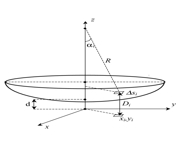
FIG. 3.: In the “proximity approximation” the force is obtained by adding the pairwise forces $\Delta f_{i}$ between opposing surface elements separated by distance $D_{i}$.

Let us consider now an ellipsoidal tip surface having two different curvatures in perpendicular directions. In the vicinity of a sample the equation describing this surface involves a quadratic dependence on $x$ and $y$:

$$z(x,y)={x^{2}\over 2R_{x}}+{y^{2}\over 2R_{y}}\ ,$$ (26)

where $R_{x}$ and $R_{y}$ are the radii of curvature in the two directions. Our previous considerations may be repeated with the modification that the tip-surface distance $D_{i}$ is now taken to be

$$D_{i}=d+z(x_{i},y_{i})\ .$$ (27)

For the purpose of integration it is useful to introduce the change of variables

$$x=(R_{x}/R_{y})^{1/2}x^{\prime}\ ,\ \ \ \ y=(R_{y}/R_{x})^{1/2}y^{\prime}\ ,$$ (28)

in terms of which the problem is effectively reduced to the spherical case, and the force for the ellipsoidal tip is given by Eq. (25) with $R=(R_{x}R_{y})^{1/2}$.

The calculations of Joule loss in the case of a spherical tip proceed as outlined in the previous section. The surface charge density of the sample for the moving cantilever now depends on both $x$ and $y$:

$$\sigma(x,y,t)={VR/2\pi\over 2dR+[x-X(t)]^{2}+y^{2}}\ .$$ (29)

The additional surface charge $\sigma^{\prime}$ that generates dissipative currents in the sample is

$$\sigma^{\prime}(x,y)=-{1\over 2\pi\mu}{\partial\over\partial t}\sigma(x,y,t)\ ,$$ (30)

and the electric field responsible for dissipation is determined from $\sigma^{\prime}$ by

$${\bf E}^{\prime}({\bf r},t)=-\nabla\int d{{\bf r}}_{\perp}{\sigma^{\prime}({{\bf r}}_{\perp})\over|{\bf r}-{\bf r}_{\perp}|}\ ,$$ (31)

where ${\bf r}=(x,y,z)$ and ${{\bf r}}_{\perp}=(x,y)$. The expression for the Joule loss is

$$W_{j}={(VX_{0}\omega)^{2}R^{1/2}\over 32\sqrt{2}\pi^{3}\mu d^{3/2}}I\ ,$$ (32)

where the (dimensionless) integral $I$ is given by

$$I=\int\int d{\bf r}_{\perp}d{\bf r}^{\prime}_{\perp}|{\bf r}_{\perp}-{\bf r}^{\prime}_{\perp}|^{-1}{\partial\over\partial x}(1+r^{2}_{\perp})^{-1}{\partial\over\partial x^{\prime}}(1+r^{{}^{\prime}2}_{\perp})^{-1}\approx 4.8\ .$$ (33)

The $d^{-3/2}$ dependence of $W_{j}$ on $d$ given by Eq. (32) is somewhat weaker than in the cylindrical case, and is comparable to the dependence on $d$ of the frictional force observed by Stipe, et al. [1]. However, the numerical value given by Eq. (32) is too small to explain the experimental results. This question will be taken up in Section 6.

IV Casimir force

The “proximity approximation” employed in the previous section can be applied to the case of the Casimir attraction. We consider the case of small separations $d$ such that $d\ll c/\omega_{p},\hbar c/k_{B}T$, where $\omega_{p}$ is the plasma frequency; $\omega_{p}\approx 10^{16}$ s^-1 for good metals, so that we require $d\ll 30$ nm. For these small separations we can use the Lifshitz formula [5] for the force per unit area:

$$f(d)={\hbar\over 8\pi^{2}d^{3}}\int d\xi{[\epsilon(i\xi)-1]^{2}\over[\epsilon(i\xi)+1]^{2}}\ ,$$ (34)

where $\epsilon$ is the dielectric permittivity, assumed to be the same for both plates. The explicit form of $\epsilon$ in the Drude approximation is

$$\epsilon(i\xi)=1+{\omega_{p}^{2}\over\xi(\xi+\nu)}\ ,$$ (35)

where $\nu$ is the electron collision frequency ($\approx 10^{13}$ s^-1 at $T=300$K), which is much smaller than $\omega_{p}$, and can be neglected when integrating Eq. (34). It follows from Eqs. (34) and (35) that

$$f(d)={\hbar\omega_{p}\over 32\sqrt{2}\pi d^{3}}\ .$$ (36)

Using (36), (22), and (24), we obtain

$$T(d)={R\hbar\omega_{p}\over 32\sqrt{2}d^{2}}$$ (37)

for a spherical tip of radius $R$. In the case of a cylindrical tip we have

$$T(d)={3bR^{1/2}\hbar\omega_{p}\over 2^{8}d^{5/2}}\ .$$ (38)

This differs from the force obtained for the case of a cylinder in Reference [14] ($T(d)\propto d^{-(n-1)},\ n=3$ or 4). The latter result was obtained using the unjustified assumption that the Casimir force satisfies Laplace’s equation in the gap between the metals. It is seen from Eqs. (37) and (38) that the dependence of the Casimir force on $d$ is stronger than in the electrostatic case. At small values of $d$ the Casimir force can be dominant.

V Attraction due to spatial fluctuations of electrostatic charge

In this section we consider a substrate with a stationary, inhomogeneous distribution of the electric charge, which can occur in good dielectrics. Such a situation was approximated experimentally [1] by employing a fused silica sample irradiated with $\gamma$ rays. In the course of irradiation, positively charged centers (Si dangling bonds) are generated. Randomly distributed positive charges are embedded in a negative background, and on average the sample is electrically neutral. We model the sample as consisting of microscopically small volume elements $\Delta V_{i}$. Each element is chosen sufficiently small that not more than one charge center is present in it. The electric charge $q_{i}$ of each element can be described by

$$q_{i}=n_{i}e+(1-n_{i})e_{b}\ ,$$ (39)

where $n_{i}=1$ or 0 for an occupied or unoccupied charge center element, respectively, and $e_{b}$ is the background charge in the volume $\Delta V_{i}$. It follows from Eq. (39) that the condition of charge neutrality, $\langle q_{i}\rangle=0$, is satisfied when

$$e_{b}=-{e\langle n_{i}\rangle\over 1-\langle n_{i}\rangle}\approx-en\ ,$$ (40)

where $n\equiv\langle n_{i}\rangle$, $n\ll 1$. In the following we will consider the fluctuations of charges in different volume elements $i,j$ to be statistically independent, so that $\langle\delta q_{i}\delta g_{j}\rangle=0$ for $i\neq j$. The mean square of charge fluctuations within a given volume element is given by

$$\langle\delta q_{i}\delta q_{i}\rangle=\langle n_{i}^{2}\rangle e^{2}+2ee_{b}\langle n_{i}(1-n_{i})\rangle+\langle(1-n_{i})^{2}\rangle e_{b}^{2}\ .$$ (41)

It follows from the definition of $n_{i}$ that $n_{i}^{2}=n_{i}$, $(1-n_{i})^{2}=1-n_{i}$, and $n_{i}(1-n_{i})=0$. Then using the assumption that $n\ll 1$, we obtain from Eq. (41) the mean square

$$\langle\delta q_{i}\delta q_{i}\rangle\approx ne^{2}\ ,$$ (42)

which shows that a random charge distribution is consistent with Poisson statistics. Each individual charge $q_{i}$ has its own image $-q_{i}$ in the bulk of the cantilever tip. Then, in the absence of cross terms, an average tip-sample attractive force is determined by adding the contributions from all the charge-image pairs. Thus the electrostatic attraction $\Delta f_{i}$ between opposing elements $\Delta V_{i}$ is given by

$$\Delta f_{i}={ne^{2}\over 4[D(x_{i},y_{i})-z_{i}]^{2}}\ ,$$ (43)

where the coordinates $x_{i}$, $y_{i}$, $z_{i}$ give the position of the $i$th volume element in the substrate, and the total force is obtained by summing over all the elements:

$$T={ne^{2}\over 4}\sum_{i}{1\over[D(x_{i},y_{i})-z_{i}]^{2}}\ .$$ (44)

After replacing the sum by an integral ($n\sum\rightarrow c\int d^{3}r$, where $c$ is the number of charge centers per unit volume), we obtain, after integration over $z$,

$$T={ce^{2}\over 4}\int\int{dxdy\over D(x,y)}={\pi ce^{2}R^{2}\over 2d}\int{d\alpha\alpha\over 1+{\alpha^{2}R\over 2d}}\ .$$ (45)

The integral on the right-hand side is logarithmically divergent. Hence we should confine the integration to values of $\alpha$ up to $\alpha_{max}\approx R_{tip}/2R$, where $R_{tip}$ is the characteristic size of the bottom part of the tip. The value of the integral is not very sensitive to $R_{tip}$, so that we may set $R=R_{tip}$. Then the force of attraction is given by

$$T={1\over 2}\pi ce^{2}R\ln\left[1+{R\over 8d}\right]\ .$$ (46)

To illustrate the importance of this force, we put in Eq. (46) the typical values $c=10^{18}$ cm^-3 (as in [1, 25], see also references therein) for the defect concentration, and $R\approx 1$ $\mu$m, $d=20$ nm. In this case the ratio of the force (46) to the Casimir force (37) is $10$. This ratio decreases with decreasing $d$.

FIG. 4.: Transverse displacement $X(z,t)$ of the cantilever centerline. Restoring force $X^{\prime}T$ acts on the tip when $\alpha\neq 0$.

Our considerations in this section have ignored the screening of the electric field in the dielectric substrate. This can be justified in the case of very small tip-sample separations (substantially smaller than screening length), as only defects in the surface layer of thickness $d$ contribute to the integral in Eq. (45). When the screening is important, the effective electric field inducing image charge in the metal is decreased by the factor of $(\epsilon+1)/2$ (see Reference [24]). This factor is equal to 2.5 in the case of silica. In addition, the tip image charge induces another image charge in the dielectric, and so forth. Nevertheless, for rough estimates it is sufficient to consider only the first pair of charges, equal to $\pm{2e/(\epsilon+1)}$.

VI Influence of attractive force on cantilever eigenfrequencies

When the cantilever geometry satisfies the conditions $L\gg b\gg a$ we can employ the equation of elasticity [27] to describe the dynamics. In the case of an isotropic material, the transverse displacement $X(z,t)$ of the beam centerline (along the $x$ axis, see Figure 4) satisfies the differential equation

$$\rho_{c}S{\partial^{2}\over\partial t^{2}}X(z,t)=-EI_{i}{\partial^{4}\over\partial z^{4}}X(z,t)\ ,$$ (47)

where $\rho_{c}$ is the density of the cantilever material, $S=ab$ is the cross-section area, $E$ is Young’s modulus, and $I_{i}=a^{3}b/12$ is the bending moment of inertia. The clamped end, at $z=0$, imposes the boundary conditions $X(z=0)=X^{\prime}(z=0)=0$. The free end at $z=L$ imposes the boundary conditions $M_{y}\equiv EI_{i}X^{\prime\prime}=0$ and $F_{x}\equiv-EI_{i}X^{\prime\prime\prime}=0$, where $M_{y}$ and $F_{x}$ are the moment of the elastic force and the elastic force in the $y$ and $x$ directions, respectively. The fundamental eigenfunction is given by $X(z,t)=X_{0}(z)\cos(\omega t)$, where

$$X_{0}(z)=A[(\cos\kappa L+\cosh\kappa L)(\cos\kappa z-\cosh\kappa z)+(\sin\kappa L-\sinh\kappa L)(\sin\kappa z-\sinh\kappa z)]\ .$$ (48)

Here $A$ is a constant, $\kappa^{4}=\omega^{2}\rho_{c}S/EI_{i}$, and

$$\omega=(3.516/L^{2})(EI_{i}/\rho_{c}S)^{1/2}\ .$$ (49)

To estimate $\omega$ we put $a=250$ nm, $b=7\times 10^{3}$ nm, $L=250$ $\mu$m, and use the material constants of Si: $\rho_{c}=2.33$ g cm^-3, $E=9\times 10^{11}$ g cm^-1 s^-2. Then we have $\omega/2\pi\approx 4\times 10^{3}$ s^-1, which is approximately the same as the value quoted in Reference [1].

In the presence of a stretching force $T$, Eq. (47) is modified to [27]

$$\rho_{c}S{\partial^{2}\over\partial t^{2}}X(z,t)=-EI_{i}{\partial^{4}\over\partial z^{4}}X(z,t)+T{\partial^{2}\over\partial z^{2}}X(z,t)\ .$$ (50)

Furthermore the boundary condition at $z=L$ ($X^{\prime\prime\prime}=0$) should be replaced by the more general condition $-EI_{i}X^{\prime\prime\prime}+TX^{\prime}=0$. The term $TX^{\prime}$ describes the effect of the restoring force when there is a nonvanishing angle between $T$ and the centerline direction at $z=L$ (see Figure 4). This value of the restoring force is valid in the case of small angles $\alpha$, when $\sin\alpha\approx\tan\alpha=-X^{\prime}(L)$.

The eigenfunctions of Eq. (50) are determined by

$$X_{0}(z) = A[(\Lambda^{2}\cos\lambda+\lambda^{2}\cosh\Lambda)(\cos\lambda z-\cosh\Lambda z)$$ (51)

$$+ (\Lambda\sin\lambda-\lambda\sinh\Lambda)(\Lambda\sin\lambda z-\lambda\sinh\Lambda z)],$$ (52)

where

$$\Lambda=L[(\tau/2)^{2}+(\kappa^{4}+\tau^{2}/4)^{1/2}]^{1/2}\ ,\ \ \ \lambda=L[(-\tau/2)^{2}+(\kappa^{4}+\tau^{2}/4)^{1/2}]^{1/2}\ ,\ \ \ \tau=T/EI_{i}\ .$$ (53)

For simplicity the coordinate $z$ in Eq. (52) is given in units of $L$. The value of $\kappa$ in Eq. (53) obeys the following eigenvalue equation:

$$2\kappa^{4}+(\tau^{2}+2\kappa^{4})\cos\lambda\cosh\Lambda+\kappa^{2}\tau\sin\lambda\sinh\Lambda=0\ .$$ (54)

The minimum value of $\kappa$ ($\kappa_{min}$) that obeys Eq. (54) determines the fundamental eigenfrequency and the explicit form of the fundamental eigenfunction (52).

In the general case the fundamental frequency is a function of the tip-sample separation, bias voltage $V$, tip geometry, and concentration of charge centers via the attraction force $T(V)$. In the case of attraction due only to an external bias voltage, there is a quadratic dependence of $T$ on $V$. The proportionality coefficient depends on the geometry of the tip-sample system. To illustrate the $\omega(V)$ dependence we use the parameters given at the beginning of this section. The results of numerical calculations are shown in Figure 5 for a cylindrical geometry and for the same parameters assumed as at the beginning of this section. It is seen that the bias voltage can have a considerable effect on the frequency shift.

FIG. 5.: Numerical results for the cantilever frequency $\omega$ and effective mass $m_{eff}$ as a function of the bias voltage $V$ in the case of a cylindrical tip (see text).

In the limit of very large $V$ (when $TL^{2}/(EI_{i})\gg 1$), the first term on the right-hand side of Eq. (50) can be omitted, and Eq. (50) is transformed into the equation for the vibration of a string. In this case, a linear dependence of $\omega$ on $V$ ($\omega\propto V/L$) should occur.

Along with the resonant frequency, the cantilever effective mass also depends on $V$. The effective mass $m_{eff}$ is the coefficient entering the oscillator equation

$$m_{eff}{\partial^{2}X(t)\over\partial t^{2}}+\Gamma{\partial X(t)\over\partial t}+kX(t)=0$$ (55)

as a parameter that determines the inertial force. ($\Gamma$ is a friction coefficient, $k$ a spring constant, and $X(t)$, as previously, is the coordinate of the tip.) The mass $m_{eff}$ is related to the coefficients in Eq. (50). This relation can be obtained from the requirement that the kinetic energy of the flexible beam equals that of the oscillator, the two being one and the same physical quantity. This condition defines $m_{eff}$ as

$$m_{eff}=\rho_{c}S\int_{0}^{L}dzX_{0}^{2}(z)/X_{0}^{2}(L)\ ,$$ (56)

where $X_{0}(z)$ is given by Eq. (52).

Thus $m_{eff}$ depends on the variation of $X$ with $z$, which in turn depends on the stretching force $T$ and the other parameters in Eq. (50). In the simplest case $T=0$, we have $m_{eff}=\rho_{c}LS/4$, i.e., a quarter of the beam’s actual mass. In general the possible variation of $m_{eff}$ should be taken into account when the friction coefficient $\Gamma$ is obtained experimentally from the relation $\Gamma=m_{eff}\omega/Q$, where $Q$ is the quality factor. In other words, not only the quality factor and the eigenfrequency, but also the value of $m_{eff}$ is required to obtain $\Gamma$. The dependence $m_{eff}(V)$ is shown in Figure 5. It is seen to be similar to that of $\omega(V)$ at small values of $V$.

Figure 6 shows the effect of the Casimir force on the fundamental frequency in the case of a spherical tip. The three curves illustrate the tendency of $\omega(d,R)$ to increase with the attractive force, which varies with $d$ and $R$ as $T\sim R/d^{2}$ (see Eq. (37)). The frequency shift observed in Reference [1] at $d=2$ nm for a gold sample corresponds to the curve $R=0.5$ $\mu$m in Figure 6. When we use the experimental value 1 $\mu$m of the radius of curvature in the $y$ direction, and set the radius of curvature in the $x$ direction equal to the cantilever thickness $a=0.25$$\mu$m, we obtain $R_{exp}=(R_{x}R_{y})^{1/2}=0.5$ $\mu$m., i.e., $R_{exp}=R$. Hence the frequency shift observed by Stipe et al. [1] (see Figure 2c of Reference [1]) may be attributable to the Casimir effect.

FIG. 6.: Effect of Casimir force on the frequency $\omega$. Solid line: $R=0.5$ $\mu$m; dashed line: $R=1$ $\mu$m; dotted line: $R=2$ $\mu$m

It is interesting to compare the experimental and theoretical values of $\Gamma$. The Joule loss $W_{j}$ [see Eqs. (13), (21), and (32)] determines the friction coefficient: It follows from energy conservation and Eq. (55) that

$$\Gamma=\frac{2W_{j}}{\omega^{2}X_{0}^{2}}.$$ (57)

In the case of the cylindrical tip we have, from Eqs. (14) and (57),

$$\Gamma=\frac{bV^{2}}{2^{6}\pi\mu d^{2}}\ .$$ (58)

Putting, as previously, $b=7\times 10^{-4}$ cm, a conductivity $\mu=4\times 10^{17}$ s^-1 for gold at 300 K, $d=20$ nm, and $V=1$ Volt, we have $\Gamma=2.4\times 10^{-20}$ kg/s, which is much smaller than the experimental value of $3\times 10^{-12}$ kg/s. For the more realistic case of a spherical tip with $R=1$ nm, our estimate for $\Gamma$ using Eq. (32) is two orders of magnitude smaller than that given by (58).

VII Conclusions

The analyses presented in this paper indicate that both electrostatic forces and Casimir forces can have a strong effect on the cantilever vibrations. The cantilever eigenfrequencies depend on the attractive force $T$, which is very sensitive to the tip geometry for small values of the tip-sample separations $d$. The effect of various forces on the cantilever eigenfrequencies appears to us to be an important consideration for the practical utilization of cantilever-based devices. It has served as a motivation in this paper to study the tip-sample interaction in some detail.

We have shown that, for small separations, $T$ depends on the shape of the cantilever tip. The dependence of $T$ on the separation $d$ is different for cylindrical and spherical tips. Thus, in the case of the electrostatic force due to a bias voltage, the attractive force varies as $d^{-3/2}$ and $d^{-1}$ for cylindrical and spherical tips, respectively. In the case of the Casimir force the dependence of $T$ on $d$ was found to be $d^{-5/2}$ and $d^{-2}$, respectively, for the cylindrical and spherical tips. We have shown that the Casimir force is responsible for the frequency shift, which is of the same order as that obtained experimentally in [1] ($\approx 4.5$ %) for a gold sample at small separation $d=2$ $nm$.

The attractive force depends furthermore on the radii of curvature, and our analysis allows for the possibility that the radii may be different in different directions. In principle, any variations of tip geometry (for instance, due to adsorption of new molecules or blunting after contact with a sample) may be detected by measurements of the frequency shift, and our theory, which connects the variations of the attractive force with the frequency shift, could be helpful in estimating the character and scale of these variations.

We have calculated the attractive force between a system of randomly distributed positive charges, embedded in a negatively charged background, and a metal tip. In the case of an electrically neutral system, only the attraction between each charge and its image contributes to the total force. This is a spatially fluctuating interaction because the overall force is linear (not quadratic) in the concentration of elementary charges. Our estimates, based on the assumption of an uncorrelated distribution of charge centers in the bulk of the substrate, indicate that the fluctuating force exceeds the Casimir force for parameters appropriate to the experiments reported in Reference [1], which employed irradiated silica as a substrate.

We have derived analytical expressions for Joule losses in a metal substrate. The Joule mechanism does not explain the cantilever damping measured in [1], but our analysis may nevertheless be useful for other systems with high-resistivity substrates.

REFERENCES

- [1] B.C. Stipe, H.J. Mamin, T.D. Stowe, T.W. Kenny, and D. Rugar, Phys. Rev. Lett. 87, 096801 (2001).
- [2] R.D. Young and H.E. Clark, Phys. Rev. Lett. 17, 351 (1966).
- [3] N.A. Burnharm, R.J. Colton, and H.M. Pollock, Phys. Rev. Lett. 69, 144 (1992)
- [4] C.C. Speake and C. Trenkel, Phys. Rev. Lett. 90, 160403 (2003).
- [5] E.M. Lifshitz, Zh. Exp. Teor. Fiz. 29, 94 (1955) [Sov. Phys. JETP, 2, 73 (1956)].
- [6] S.K. Lamoreaux, Phys. Rev. Lett. 78, 5 (1997).
- [7] U. Mohideen and A. Roy, Phys. Rev. Lett. 81, 4549 (1998).
- [8] H.B. Chan, V.A. Aksyuk, R.N. Kleiman, D.J. Bishop, and F. Capasso, Phys. Rev. Lett. 87, 21 (2001).
- [9] G. Bressi, G. Carugno, R. Onofrio, and G. Ruoso, Phys. Rev. Lett. 88, 041804 (2002).
- [10] M. Bordag, U. Mohideen, and V.M. Mostepanenko, Phys. Rep. 353, 1 (2001).
- [11] P.W. Milonni, The Quantum Vacuum: An Introduction to Quantum Electrodynamics, Academic Press, New York, 1994.
- [12] K.A. Milton, The Casimir Effect: Physical Manifestations of Zero-Point Energy, World Scientific Publishing Co., Singapore, 2001.
- [13] I. Dorofeyev, H. Fuchs, G. Wenning, and B. Gotsmann, Phys. Rev. Lett. 83, 2402 (1999).
- [14] I. Dorofeyev, H. Fuchs, B. Gotsmann, and G. Wenning, Phys. Rev.B 60, 9069 (1999).
- [15] A.I. Volokitin and B.N. Persson, Phys. Rev. B65, 115419 (2002).
- [16] B. Gotsmann and H. Fuchs, Phys. Rev. Lett. 86, 2597 (2001).
- [17] P. Mohanti, D.A. Harrington, K.L. Ekinci, Y.T. Yang, M.J. Murphy, and M.L. Roukes, Phys. Rev.B 66, 085416 (2002).
- [18] J.B. Pendry, J. Phys.: Condens. Matter 9, 10301 (1997)
- [19] B.N.J. Persson and Z. Zhang, Phys. Rev.B 57, 7327 (1998).
- [20] A.I. Volokitin and B.N.J. Persson, J. Phys.: Condens. Matter 11, 345 (1999).
- [21] D. Robaschik and E.Wieczorek, Ann. Phys. 236, 43 (1994).
- [22] D. Robaschik and E. Wieczorek, Phys. Rev. D 52 2341 (1995).
- [23] G. Barton, J. Phys. A: Math. Gen. 24, 991 (1991).
- [24] L.D. Landau and E.M. Lifshitz, Electrodynamics of Continuous Media (Pergamon Press, London, 1960).
- [25] B.C. Stipe, H.J. Mamin, C.S. Yannoni, T.D. Stowe, T.W. Kenny, and D. Rugar, Phys. Rev. Lett. 87, 277602 (2001).
- [26] T.H. Boyer, Phys. Rev. A9,68 (1974).
- [27] L.D. Landau and E.M. Lifshitz, Theory of Elasticity (Pergamon Press, London, 1970). instance, XXX.