Generating droplets in two-dimensional Ising spin glasses by using matching algorithms

Abstract

We study the behavior of droplets for two dimensional Ising spin glasses with Gaussian interactions. We use an exact matching algorithm which enables study of systems with linear dimension $L$ up to 240, which is larger than is possible with other approaches. But the method only allows certain classes of droplets to be generated. We study single-bond, cross and a category of fixed volume droplets as well as first excitations. By comparison with similar or equivalent droplets generated in previous works, the advantages but also the limitations of this approach are revealed. In particular we have studied the scaling behavior of the droplet energies and droplet sizes. In most cases, a crossover of the data can be observed such that for large sizes the behavior is compatible with the one-exponent scenario of the droplet theory. Only for the case of first excitations, no clear conclusion can be reached, probably because even with the matching approach the accessible system sizes are still too small.

I Introduction

Ising spin glasses are amongst the most-frequently studied systems in statistical physics reviewSG . However, despite more than two decades of intensive research, many properties of spin glasses, especially in finite dimensions, are still not well understood. For two-dimensional Ising spin glasses it is now widely accepted that no ordered phase for finite temperatures exists rieger1996 ; kawashima1997 ; stiff2d ; houdayer2001 ; carter2002 . For $d=2$ the behavior is usually described by a zero-temperature droplet scaling (DS) approach McM ; BM ; FH .

The droplet picture assumes that the low-temperature behavior is governed by droplet-like excitations, where excitations of linear spatial extent $l$ typically cost an energy of order $l^{\theta}$. These excitations are expected to be compact and their surface has a fractal dimension $d_{s}<d$, where $d$ is the space dimension. Furthermore it is usually assumed that the scaling behavior of the energy $\delta E$ of different types of excitations, e.g. droplets and domain walls, induced by changing boundary conditions, are described by the same exponent $\theta$.

The value of $\theta$ for domain walls in systems with Gaussian disorder has been determined by several studies bray1984 ; mcmillan1984b ; rieger1996 ; palassini1999a ; stiff2d ; carter2002 with results close to the most recent result aspect-ratio $\theta=-0.287(2)$. For simplicity, we will assume $\theta=-0.29$ from now on. On the other hand, in a previous study of droplets by Kawashima and Aoki KA using Monte Carlo simulations of moderate sized systems, a different exponent $\theta=-0.45(5)$ was found. Note that droplets can be generated by using several methods, and the resulting scaling behavior may in principle depend on the droplet type considered. By using exact ground-state (GS) algorithms opt-phys2001 , so called matching algorithms (see Sec. II), one can study much larger system sizes than is possible with other approaches. On the other hand matching algorithms are less flexible than Monte Carlo methods, and not all types of droplets can be generated using them. But recently, through the application of an extended matching algorithm droplets , we were able to generate the same type of droplets as in Ref. KA, but for much larger systems. For large systems, the value $\theta=-0.29$ of the exponent was again found. To be precise, the scaling of the droplet energies exhibited a crossover of the form

$$\Delta E=Al^{\theta}+Bl^{-\omega}.$$ (1)

with $\theta=-0.29$, $\omega=1$, while for small sizes, the behavior was compatible with an apparent exponent of $\theta^{\prime}=-0.47(1)$. Hence the predictions of DS have been verified for this type of droplet, simply by studying larger system sizes.

Recently, the same crossover phenomenon was sought by Berthier and Young berthier2003 when studying droplets, obtained by a Monte Carlo minimization in a system with size $L=64$ while fixing the size of the droplets to either one value or to a range of values. In both cases, for the largest droplets, the scaling was determined by an exponent resembling the domain-wall exponent, i.e. close to $\theta=-0.23$. But only for the second type of droplets with a range of sizes could a crossover phenomenon be observed, and then it only occurred for very small droplets. For a third type of droplet, no crossover and a scaling exponent $\theta=-0.32$ close to the domain-wall value was found excited2d .

On the other hand, Picco, Ritort and Sales picco2001 ; picco2003 have studied the lowest excitation in systems with sizes up to $L=16$ using a transfer matrix approach. Through a scaling argument connecting lowest excitations to droplets (see Sec. V), their result implied $\theta=-0.47$.

In order try to clarify the above mentioned results and relate them to our previous results droplets we study in this paper different types of droplets by applying again the matching algorithm. This allows us to go to larger sizes than in the studies where no matching algorithm was applied. On the other hand, the matching algorithm is less flexible and enables us to generate only certain types of droplets. Where differences in the scaling behavior arise amongst the various droplet types we shall attempt to understand their origin.

The Hamiltonian which is studied here is the usual Ising spin glass model:

$${\mathcal{H}}=-\sum_{\langle i,j\rangle}J_{ij}S_{i}S_{j},$$ (2)

where the sites $i$ lie on the sites of a square lattice with $N=L^{2}$ sites, $S_{i}=\pm 1$, the $J_{ij}$ have a Gaussian distribution of zero mean and unit variance and couple nearest-neighbor sites on the lattice.

In the next section, we will outline how the matching algorithm works and how the droplets are generated. In the main four sections of this paper, four different types of droplets are studied, their scaling behavior is investigated and compared to previous results, if available. In the last section, a summary and an outlook are given.

II Algorithm

The GS problem for general spin glasses is NP-hard SG-barahona82 . This means that only algorithms are known, where the running time in the worst case increases exponentially with the system size garey1979 . Hence, only small systems can be studied in the general case. For the special case of two-dimensional spin glasses without an external field and with periodic boundary conditions in at most one direction, i.e. for planar graphs, efficient polynomial algorithms SG-barahona82b for the calculation of exact GSs are available. If one is interested in obtaining the partition sum, without obtaining spin configurations, one can also treat systems with full periodic boundary conditions in polynomial time, by using transfer-matrix approaches saul1993 ; saul1994 ; regge1996 ; cho1997 , but the running time is again strongly increasing, limiting the investigations to small systems. The most recent studies are based on matching algorithms SG-bendisch1991 ; SG-bendisch1992 ; SG-bendisch1994 ; SG-bendisch1995 ; SG-kisker1996 ; SG-kawashima1997 ; SG-bendisch1997 ; SG-bendisch1998 ; SG-achilles2000 , while other exact approaches can be found in Refs. SG-ozeky1990 ; SG-kadowaki1997 ; middleton2001 . Results for systems of size $1800\times 1800$ have now been obtained SG-palmer1999 !

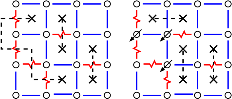
Figure 1: 2d spin glass with all spins up (left, up spins not shown). Straight lines are ferromagnetic, jagged lines antiferromagnetic bonds. The dotted lines connect frustrated plaquettes (crosses). The bonds crossed by the dotted lines are unsatisfied. In the right part the GS with three spins pointing down (all other up), corresponding to a minimum number of unsatisfied bonds, is shown

Here, just the basic idea of the matching algorithm will be explained. For the details, see Refs. bieche1980, ; SG-barahona82b, ; derigs1991, . The method works for spin glasses which are planer graphs. In the left part of Fig. 1 a small 2d system with open boundary conditions is shown. All spins are assumed to be “up”, hence all antiferromagnetic bonds are not satisfied. If one draws a dotted line perpendicular to all unsatisfied bonds, one ends up with the situation shown in the figure: all dotted lines start or end at frustrated plaquettes and each frustrated plaquette is connected to exactly one other frustrated plaquette. Each pair of plaquettes is then said to be matched. Now, one can consider the frustrated plaquettes as the vertices and all possible pairs of connections as the edges of a (dual) graph. The dotted lines are selected from the edges connecting the vertices and called a perfect matching, since all plaquettes are matched. One can assign the edges in the dual graph weights, which are equal to the sum of the absolute values of the bonds crossed by the dotted lines. The weight $\Lambda$ of the matching is defined as the sum of the weights of the edges contained in the matching. As we have seen, $\Lambda$ measures the broken bonds, hence, the energy of the configuration is given by $E=-\sum_{\langle i,j\rangle}|J_{ij}|+2\Lambda$. Note that this holds for any configuration of the spins, since a corresponding matching always exists. Obtaining a GS means minimizing the total weight of the broken bonds (see right panel of Fig. 1), so one is looking for a minimum-weight perfect matching. This problem is solvable in polynomial time. The algorithms for minimum-weight perfect matchings MATCH-cook ; MATCH-korte2000 are among the most complicated algorithms for polynomial problems. Fortunately the LEDA library offers a very efficient implementation PRA-leda1999 , except that it consumes a lot of memory, which limits the size of the systems to about $N=500^{2}$ on a typical 500 MB workstation.

For system with periodic boundary conditions in both directions, the matching approach is not feasible. Hence, we restrict the study to systems with free or with half periodic-half free boundary conditions.

To study the behavior of two-dimensional spin glasses, here not only GSs, but also low-lying excited states are generated. For this purpose GS algorithms can be used as well. The general procedure consists of these three steps:

1. Calculate the GS $\{S_{i}^{(0)}\}$ of a given realization and the GS energy $E_{0}$.

2. Modify some of the couplings so that the GS is changed.

3. Calculate the GS $\{S_{i}^{(m)}\}$ of the modified system, which is usually a low-lying excited state of the original realization. The energy of $\{S_{i}^{(m)}\}$ calculated with the original (unmodified) bonds is denoted by $E_{0}^{m}$.

In this work four different ways of generating excitations are considered. The technical details are in the corresponding sections.

• Single-bond droplets: the most straightforward implementation, where only one bond is changed with respect to the initial coupling.

• Cross droplets: This mimics the generation of droplets induced by flipping one (central) spin. It involves changing $O(L)$ bonds, iterating over $2L-2$ changes, and picking the minimum-energy excitation among them.

• First excitations: The lowest excitation above the GS is calculated. This involves the change of one bond (or $O(L)$ bonds if the boundary spins are fixed), iterating over $O(L^{2})$ changes, and picking the minimum-energy excitation among them.

• Fixed-volume droplets: The matching algorithm does not allow for fixing the size. Hence, the size constraint is imposed here, when selecting among different cross droplets of each realization.

The main quantities analyzed are the energy $\Delta E=E_{0}^{m}-E_{0}$, the volume $n$ and the surface $S$ of the droplets/excitations.

III Single-bond droplets

In Ref.KA, , droplets were generated by flipping one central spin with respect to the GS. Since matching algorithms do not allow the inclusion of external fields, this approach cannot be directly applied. The most natural and simple idea is to flip instead a central bond with respect to the GS. This is performed by introducing a hard bond, i.e. changing the value of one bond $(i_{0},j_{0})$ such that $|J_{i_{0}j_{0}}|$ is so large $|J_{i_{0}j_{0}}|=J_{\rm big}$, that it will be always satisfied in a GS, see Fig. 2. In this case the hard bond $(i_{0},j_{0})$ will be inverted, i.e. the spins $S_{i_{0}}$ and $S_{j_{0}}$ will be forced to take a relative orientation opposite to the GS, hence $J_{i_{0}j_{0}}=-J_{\rm big}S_{i_{0}}S_{j_{0}}$. The GS of the modified system now generates a minimum-energy droplet, called a single-bond droplet here, with the constraint that the surface of the droplet runs through $(i_{0},j_{0})$.

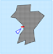
Figure 2: Method used to generate the single-bond droplets. After calculating the GS, one inverted hard bond (see triangle) generates an excitation (dark inner area).

We have studied single-bond droplets for system sizes $L=6$ to $L=240$ while averaging over more than 3000 samples for each size. In Fig. 3 the average droplet energy $\langle\Delta E\rangle$ is shown as a function of the system size $L$. A double-logarithmic plot (not shown) shows a curvature, which is not compatible with a convergence of the droplet energy to zero, but compatible with a convergence to a non-zero energy. This seems plausible, because the choice that a certain bond, i.e. the inverted hard bond in the modified system, has to belong to the minimum domain wall, imposes a penalty on the energy of the droplet. This energy should be of the order of the coupling constant $J=1$. In the spirit of Ref. droplets, , where a crossover of the cross droplet energy according to $AL^{\theta}+BL^{-\omega}$ has been observed, we have performed a fit to a function $\Delta E(L)=\Delta E_{r}+AL^{\theta}+BL^{-\omega}$ with fixing $\theta=-0.29$, resulting in $\Delta E_{r}=1.79(6)$ and $\omega=-1.8(2)$, with a fair quality of the fit goodness , $Q=0.14$. Interestingly, this is a similar correction to scaling exponent $\omega$ as found when iterating the generation of excitations over all single bonds and selecting the droplet from all excitations containing the central spin droplets . One might be tempted to conclude that these types of droplet shows a similar behavior to the cross droplets studied in Ref. droplets, , (see also the inset of Fig. 3). But the fit is not very sensitive to the choice of $\theta$. If one allows also the variable $\theta$ to adjust in the fit, $\theta=-1.01(9)$, $\Delta E_{r}=1.96(2)$ and $\omega=-6(4)$ results in $Q=0.83$. Hence, this type of droplet seems to be very different from the cross droplets studied in Ref. droplets, , (which are similar to the droplets generated by flipping a single spin within a Monte-Carlo minimization KA ).

Figure 3: Average energy of single-bond droplets. The line shows a fit to the function $\Delta E(L)=\Delta E_{r}+AL^{\theta}+BL^{-\omega}$ with $\theta=-0.29$ resulting in $\Delta E_{r}=1.79(6)$ and $\omega=-1.8(2)$. The inset shows the same data with the limiting energy $\Delta E_{r}$ subtracted in a double logarithmic plot.

This difference is visible also in the behavior of the single-bond droplet volume and surface, which are shown in Fig. 4. We have fitted to power-law functions $L^{D_{n}}$ resp. $L^{d_{S}}$ resulting in exponents $D_{n}=1.39(1)$ and $d_{S}=0.769(5)$, hence $D_{n}/d_{S}=1.8$. This means this type of droplet grows much slower than the size of the system, i.e. it is very different from growth as $L^{2}$ which was found for cross droplets droplets .

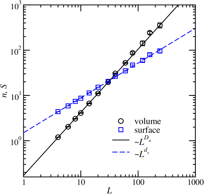
Figure 4: Average volume $n$ and average surface $S$ for the single-bond droplets as a function of the system size $L$. The straight lines represent fits to power-laws with exponents $D_{n}=1.39(1)$ resp. $d_{S}=0.769(5)$

Basically the above results mean that single-bond droplets are not the droplets which will dominate the low-temperature thermodynamics of the spin glass, due to their high energy cost as mentioned above. Therefore, other procedures have to be applied to obtain more physically relevant droplets when using a matching algorithm. However, the single-bond droplets are not without their uses, as they are the first step in obtaining the lowest energy excitations of the system, (see section V).

IV Cross droplets

The basic idea of the cross droplets is to mimic the approach, which was used by Kawashima and Aoki to obtain droplets using a Monte Carlo simulation KA . They first calculated the GS. Then they recalculated the GS with the constraints that the spins on the boundary keep their GS orientations while a central spin is flipped. Using this approach, small system up to $L=50$ could be studied, and a scaling $\Delta E\sim L^{\theta^{\prime}}$ of the droplet energy with $\theta^{\prime}=-0.45(1)$ was found.

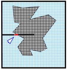
Figure 5: Method used to generate the cross droplets. After calculating the GS, several hard bonds (thick lines) are introduced, one hard bond is inverted (see triangle), leading to the appearance of an excitation (dark inner area).

Our generation of the droplets works in the following way. After obtaining the GS several hard bonds are introduced, see Fig. 5. If the subsystem of hard bonds does not exhibit frustration, no hard bond will be broken, when a new GS is calculated. First, all boundary spins are fixed relative to each other by introducing hard bonds around the border, i.e. the bonds between pairs of boundary spins are replaced. The sign of the hard bonds is chosen such that they are compatible with the GS orientations of the adjacent bonds. This keeps the spins on the boundary in their GS orientations. Second, a line of hard bonds is created which runs from the middle of (say) the left border to a pre-chosen center spin, again fixing the pair’s spins in their relative GS orientations. Next, the sign of exactly one hard bond on this line is inverted. Finally, a GS of the modified realization is calculated. With respect to the original GS, the result is a minimum energy excitation fulfilling the constraints that it contains the center spin, does not run beyond the boundary and that it has a surface which runs through the hard bond which has been inverted. The energy of the excitation is defined as the energy of the resulting configuration calculated using the original bond configuration. For each realization, this procedure is iterated over all the bonds which are located on the line from the boundary to the center, when in each case exactly one hard bond is inverted. Furthermore, this procedure is iterated over all four lines of bonds running from the left, right, top and bottom boundary to the center spin. Among all generated $2L-2$ excitations, the one exhibiting the lowest energy is selected as the cross droplet.

In a previous work droplets , we have found that the cross droplets are almost equivalent to those of Kawashima and Aoki. Indeed for the system sizes which can be studied, the difference is much smaller than the statistical error bars. It turned out that cross droplets exhibit for small sizes a power-law behavior with an effective exponent $\theta^{\prime}=-0.47$. But for large sizes a crossover to a power-law behavior is found, governed by the exponent $\theta=-0.29$, which is the same value as found in domain-wall studies bray1984 ; mcmillan1984b ; rieger1996 ; palassini1999a ; stiff2d ; carter2002 .

Now we want to compare our results with recent results on fixed-volume droplets obtained by Berthier and Young berthier2003 . They have studied the energy dependence of droplets for systems with $L=64$ when fixing the droplet size to an interval $[n,n+\delta(n)]$. They considered two cases, $\delta(n)=0$ and $\delta(n)=n-1$. For each realization, they optimized the energy of a droplet using a parallel-tempering Monte Carlo simulation. The optimization was done while observing the constraints that the center spin is included, that the size is within the given size range and that the droplet remains connected. For both cases of $\delta(n)$, they observed for larger droplets a scaling of the droplet energy which is compatible with the DS scenario, i.e. a $\Delta E\sim n^{\theta^{\star}/d_{f}}$ behavior with $\theta^{\star}=$ around -0.23 and $d_{f}=2$. For the case of fixed droplet size ($\delta(n)=0$), this behavior was found also for the smallest droplet sizes. For the fluctuating sizes ($\delta(n)=n-1$), a crossover from the small-droplet behavior with a more negative effective exponent to the large-droplet behavior was found, similar to the crossover observed before for the cross droplets droplets .

Furthermore, they have studied the distributions $P(\Delta E)$ of droplet energies. In both cases they have found that the distribution exhibits a scaling behavior according to

$$P_{L}(\Delta E)=\frac{1}{\langle\Delta E\rangle_{L}}P\left(\frac{\Delta E}{\langle\Delta E\rangle_{L}}\right)\,.$$ (3)

For the case $\delta(n)=0$ they found that $P_{L}(0)$ is zero (or very) close, while for $\delta(n)=n$ a convergence to a non-zero value was obtained.

This difference between their two droplet types motivated us to study $P(\Delta E)$ also for cross droplets. In Fig. 6 the distributions of the droplet energies for this droplet type is shown. We have studied system sizes up to $L=160$ and averaged over 5000 independent realisations in all cases. One observes that $P(0)$ is different from zero and growing with system size. The typical droplet energy, i.e. the maximum of the distribution, is at a value different from zero in the thermodynamic limit. This can be seen from Fig. 7, where the rescaled distributions $\langle\Delta E\rangle P(\Delta E)$ of the droplet energies for the cross droplet type are shown. The scaling behavior of $\langle\Delta E\rangle$ shows finite-size corrections, as discussed in Ref. droplets, . In that work, for large systems, $\langle\Delta E\rangle\sim L^{\theta}$ with $\theta\sim-0.28$ was found. Interestingly, the scaling assumption (3) seems not to work well near $\Delta E=0$, where a systematic increase of the data points with system size is found, instead of a data collapse. To investigate this effect, we have evaluated $P(0)$ as a function of system size, see inset of Fig. 7. Here again a crossover can be observed. For larger sizes, we find $P(0)\sim L^{\theta_{0}}$, with $\theta_{0}=0.45(1)$. Hence the scaling assumption $P_{L}(\Delta E)\sim\frac{1}{L^{\theta}}P(\frac{\Delta E}{L^{\theta}})$ may be wrong. But given the system sizes studied here, it cannot be excluded that for even larger sizes, $P(0)$ shows another crossover to the behavior found for the mean value $\langle\Delta E\rangle$ already at smaller systems.

To conclude, the scaling behavior of the distribution of droplet energies for the cross droplets is similar to the $\delta(n)=(n-1)$ droplets of Berthier and Young, in the sense that $P(0)$ is finite and growing. This similarity has been observed already, when studying simply the mean value $\Delta E$. On the other hand, the scaling assumption (3) seems not to work near $\Delta E=0$ in contrast to the results of Ref. berthier2003, . Thus, we have another example of the scaling behavior of droplets seemingly depending on the recipe used to generate them, at least at the system sizes which can be studied at present.

Figure 6: Distribution of droplet energies for cross droplets for system sizes $L=14,20,40,80,160$. Error bars are of the order of the symbol size (see $L=14$ datapoints). Lines are guides for the eyes only.

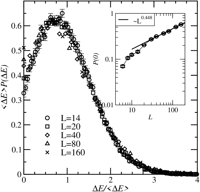
Figure 7: Rescaled distribution of droplet energies for cross droplets for system sizes $L=14,20,40,80,160$. The inset shows the probability $P(0)$ to get a zero-energy droplet as a function of system size $L$. For larger sizes, $P(0)$ scales as $L^{\theta_{0}}$ with $\theta_{0}=0.45(1)$.

V First excitations

Next, we consider the first (i.e. the lowest) excitation of the system above the ground state. They have been studied by Picco, Ritort and Sales picco2001 ; picco2003 who generated the lowest excitation for sizes up to $L=16$ using a transfer matrix method. They have measured the exponent $\theta_{1}$ describing the finite-size scaling $\Delta E\sim L^{\theta_{1}}$ of the excitation energy and the exponent $\lambda_{l}$ characterizing the size distribution of the excitation volumes $n$ according to $P(n)\sim n^{-(1+\lambda_{l})}$. Furthermore, they have derived a scaling relation $\theta=\theta_{1}+d\lambda_{l}$ ($d=2$ here), connecting the exponents to the usual droplet exponent $\theta$. Picco et al. argue $\theta_{1}=-2$ (while their numerical results are close to $\theta_{1}=-1.7(1)$, but they explain this discrepancy as due to the small sizes they could study) and they have found $\lambda_{l}=0.77(1)$, leading to $\theta=-0.46(2)$.

As we have already seen for the single-spin induced (i.e. here cross) droplets, large sizes may be needed to see the correct scaling behavior, hence $L=16$ may be much too small. To test their results for larger sizes up to $L=64$ we have also calculated first excitations by using the matching algorithm. They are obtained by iterating one hard bond over all bonds and then selecting for each realization the minimum excitation among all $O(L^{2})$ droplets. We have considered free and fixed boundary conditions. In the latter case, again a closed loop of hard bonds winds around the system. We averaged over a number of realizations ranging from a few hundred for the largest sizes to $10^{4}$ for $L\leq 12$. In Fig. 8 the average energy of the lowest excitations for both types of boundary conditions are shown. For free boundary conditions excitations leaving the boundary spins unchanged can be realized. Thus, for each system, the energy of the lowest excitation with fixed boundary conditions is an upper bound for the energy of the excitation with free boundary conditions. Furthermore, in the thermodynamic limit, the boundary conditions are expected to be irrelevant for the energies of a droplet, hence both cases should agree for $L\to\infty$. Indeed in Fig. 8, the average energy for the fixed boundary conditions is always above the average energy for droplets with free boundaries. Furthermore, both curves approach each other with growing system size. For small system sizes, the first excitations with free boundary conditions can take advantage of the system boundary, i.e. many of the droplets will run up to the boundary, where creating a domain wall does not cost energy. Hence large corrections to scaling can be expected, as is visible in the figure. In Ref. picco2001, only small systems $L\leq 12$ were considered. Hence, the corrections to scaling were hardly visible and a $L^{-1.7}$ behavior was observed.

Droplets for the case with fixed boundaries show less corrections to scaling, because the system cannot create domain walls of low energy cost. For $L\geq 10$ a fit to an algebraic decrease of the excitation energy of the form $L^{b}$ yields $b=-2.27(2)$. Since the lowest excitations for both boundary conditions have to agree for $L\to\infty$ and because the droplets with fixed boundaries exhibit almost no corrections to scaling, it can be expected that also the lowest excitations with free boundaries show the $L^{b}$ scaling for large sizes. This can be represented by a function with a $L^{b^{\prime}}/(1+eL^{b^{\prime}-b})$ scaling behavior, see Fig. 8. But the system sizes accessible to us, although much larger than those of Ref. picco2001, , are still too small to give a definite answer for this type of droplet.

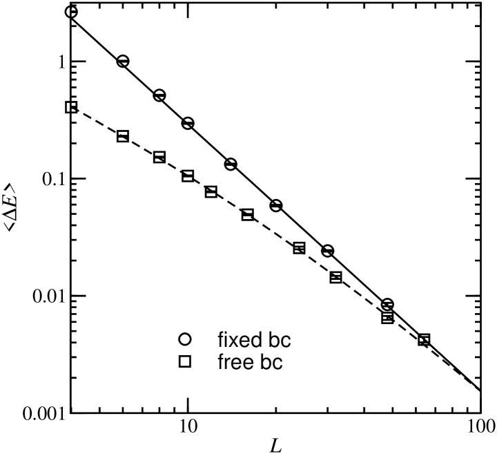
Figure 8: Average excitation energy $\Delta E$ as a function of system size for lowest excitations with free and with fixed boundary conditions. The lines denote fits to functions of the form $\Delta E_{\rm fixed}(L)=aL^{\theta_{1}}$ with $a=55(4)$, $\theta_{1}=-2.27(2)$ (fitted for $L\geq 10$) and $\Delta E_{\rm free}(L)=cL^{b^{\prime}}/(1+eL^{b^{\prime}-\theta_{1}})$ with $c=2.8(2)$, $b^{\prime}=-1.27(5)$, $e=0.041(3)$.

The fact that the droplets with free boundaries have larger finite-size corrections can be seen as well when studying the distribution of the droplet energies. In Fig. 9 the rescaled distribution $P(\Delta E)L^{\theta_{1}}$ of the droplets is displayed. For small systems a good data collapse is obtained for $\theta_{1}=-1.4$, corresponding to the slope of the mean droplet energy in Fig. 8. For larger sizes, the best data collapse is obtained for $\theta_{1}=-1.8$.

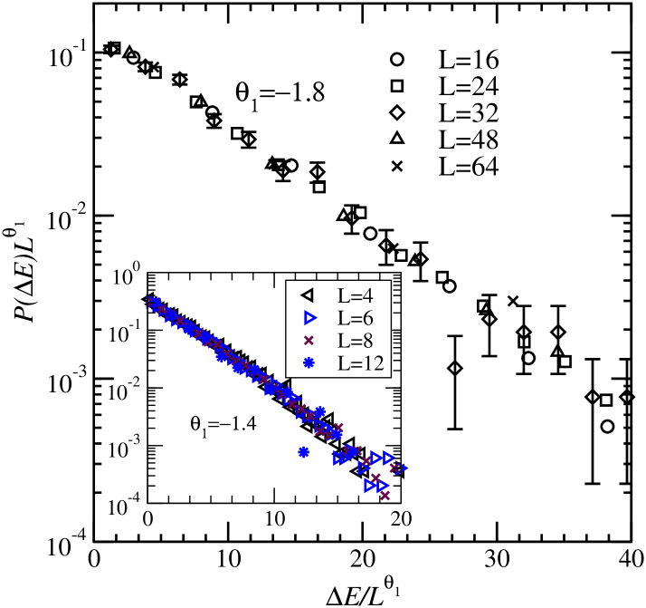
Figure 9: Rescaled distributions $P(\Delta E)L^{\theta_{1}}$ as a function of the rescaled excitation energies $\Delta E/L^{\theta_{1}}$ for the lowest excitations for free boundaries. For large system sizes $\theta_{1}=-1.8$ was used, while for small systems (see inset) $\theta_{1}=-1.4$ was applied. As an example, the error bars for $L=32$ are shown, which are large in the region of large, hence rare, energy values.

For the case of fixed boundaries, corresponding to the Fig. 8, the best data collapse $P(\Delta E)L^{\theta_{1}}$ versus $\Delta E/L^{\theta_{1}}$ is obtained for $\theta_{1}=-2.3$, see Fig. 10.

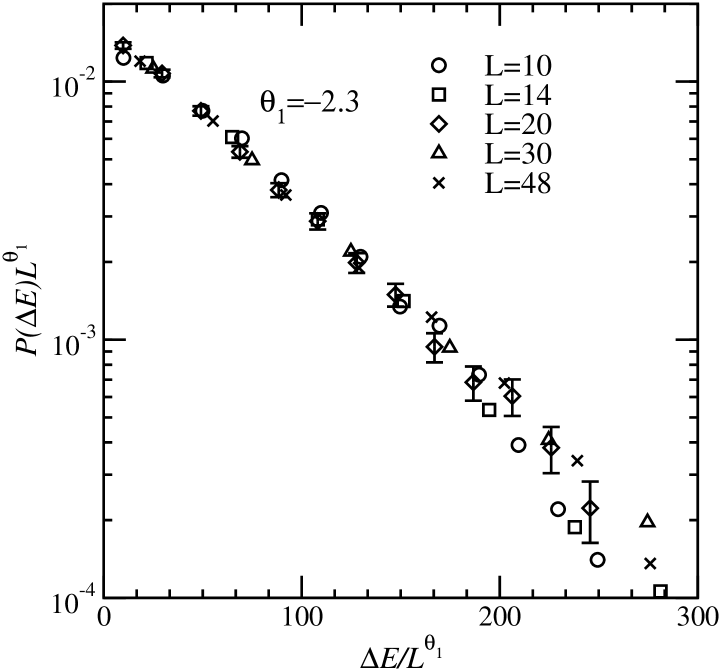
Figure 10: Rescaled distributions $P(\Delta E)L^{\theta_{1}}$ as a function of the rescaled excitation energies $\Delta E/L^{\theta_{1}}$ for the lowest excitations for fixed boundaries. $\theta_{1}=-2.3$ is used. As an example, the error bars for $L=20$ are shown.

The different values for $\theta_{1}$ for the $L^{\theta_{1}}$ scaling can be understood as follows. The lowest excitation is generated by iterating one hard bond over all bonds of a system. Then the minimum-energy droplet is taken among all this $O(L^{2})$ excitations. To the lowest order, this procedure generates droplets, where the energy scales like

$$\Delta E\sim 1/(L^{2}P^{\star}(0))\,,$$ (4)

here $P^{\star}(0)$ is the probability to obtain a (single-bond) excitation having zero energy. Hence, to understand the scaling of $\Delta E$, one should study the scaling of $P^{\star}(0)$. In Fig. 11 the distribution of energies of all single-hard-bond excitations (fixed boundary conditions) is displayed along with the finite-size behavior of $P^{\star}(0)$. For large enough sizes $P^{\star}(0)$ scales about as $L^{0.3}$ leading to $\Delta E\sim L^{-2.3}$ as found in the data. Hence, the scaling $P^{\star}(0)$ for the single-bond excitations is compatible with a $P^{\star}(0)\sim 1/L^{\theta}$ behavior with $\theta\approx-0.3$, yet again the value found from domain wall studies.

Note that for small sizes, $P^{\star}(0)$ grows more rapidly than at larger sizes, while from the scaling behavior of $\langle\Delta E\rangle$, the opposite would be expected. This deviation is presumably due to the fact that for small sizes the behavior of the energy distribution a little bit away from $\Delta E=0$ contributes as well. In this region it was assumed when deriving Eq. (4), that the distribution is constant, so ($P^{\star}(\Delta E^{\star})\sim P^{\star}(0)$) for small energies, which is, as visible in Fig. 11, not the case. It is only for larger sizes that the scaling behavior at $\Delta E=0$ is relevant, leading to the expected result.

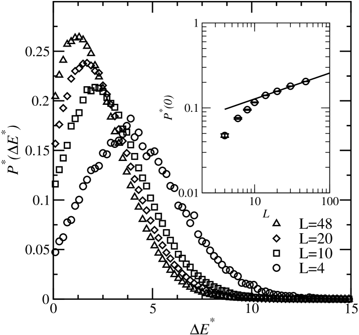
Figure 11: Distribution $P^{\star}(\Delta E^{\star})$ of single-bond excitations energies with fixed boundary condition when iterated over all bonds of each realization, for system sizes $L=4,10,20,48$. The inset shows the finite-size behavior of $P^{\star}(0)$. The line in the inset represents a $L^{0.3}$ behavior.

In Fig. 12 the corresponding distribution of energies for the excitations with free boundary conditions is shown. As one can see, excitations having zero energy are much more likely than in the fixed boundary case, because they can take advantage of letting the domain wall end at the boundary. For small sizes $P^{\star}(0)$ is slightly decreasing, corresponding to the moderate decrease of $\langle\Delta E\rangle$ seen in Fig. 8, while for moderate sizes, $P^{\star}(0)$ is constant as a function of system-size, indeed compatible with $\theta_{1}=-2$, as argued by Picco et al. Note that here the scaling of $\langle\Delta E\rangle$ is also for small sizes compatible with the scaling of $P^{\star}(0)$, because here $P^{\star}(\Delta E^{\star})$ is much more constant near $\Delta E^{\star}=0$ and $P^{\star}(0)$ is much larger.

For larger system sizes, when the system boundary is far away, the behavior of $P^{\star}(0)$ for the two cases of boundary conditions should agree again. Unfortunatly, although the matching algorithm is a very powerful tool, these sizes are out of reach with current technology. Hence it is hard to say, whether $P^{\star}(0)\sim L^{0.3}$ or $P^{\star}(0)$ constant is the true limiting behavior

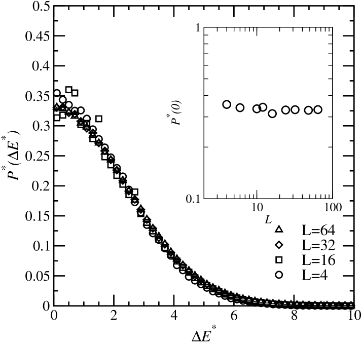
Figure 12: Distribution $P^{\star}(\Delta E^{\star})$ of single-hard-bond excitations energies with free boundary conditions when iterated over all bonds of each realization, for system sizes $L=4,16,32,64$. The inset shows the finite-size behavior of $P^{\star}(0)$.

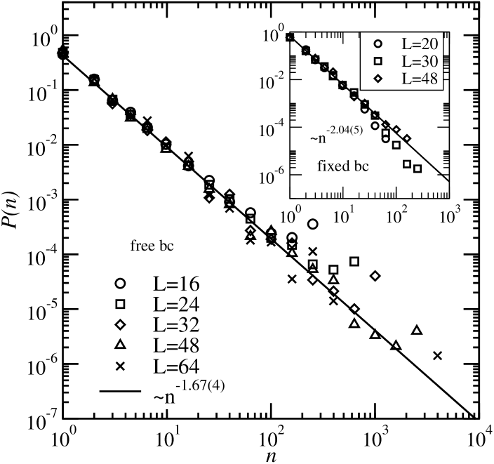
Figure 13: Distributions $P(n)$ of excitation volumes for lowest excitations with free boundary conditions for different system sizes $L=16,24,32,48,64$. Apart from the largest volumes, where the excitations start to touch the boundary, the data is very well described by a power-law behavior $n^{-1-\lambda_{l}}$ with $\lambda_{l}=0.67(4)$ from a fit to the $L=48$ data in the range $n\in[1,1000]$. The inset shows the same distribution for the case of fixed boundary conditions. The line represents in this case a power law with $\lambda_{l}=1.04(5))$.

Finally, to complete our comparison with the results of Ref. picco2003, , we show in Fig. 13 the distributions of excitation volumes for the lowest excitations for both types of boundary conditions. It exhibits a $P(n)\sim n^{-(1+\lambda_{l})}$ behavior picco2003 , except for the largest sizes, where the excitations start to interact with the system boundary. We have fitted power-laws to our data, ignoring the data points for the largest sizes and obtained $\lambda_{l}=0.67(4)$ for free bc and $\lambda_{l}=1.04(5)$ for fixed bc. The former value is compatible with the previous result $\lambda_{l}\approx 0.7$ obtained from direct finite-size scaling picco2003 , while the final value quoted in this reference is $\lambda^{\rm eff}=0.77$ obtained from an aspect-ratio analysis, i.e. using non-square systems.

Anyway, it seems strange that in both cases no large size-dependence of $\lambda_{l}$ is visible. Since one would again expect that in the thermodynamic limit results obtained from both types of boundary conditions should agree, one would expect that the behavior of one of the distributions should converge to the behavior of the other.

To summarize, for the behavior of the mean value $\langle\Delta E\rangle$, the free-boundary case exhibits a strong size dependence, while the fixed-boundary case exhibits almost none. Hence in this case one would expect that for large sizes the free-boundary case seems converged to the fixed-boundary results. When studying $P^{\star}(0)$, both cases show a crossover, hence it seems possible that one or both exhibit another crossover, leading to the same thermodynamic limit. Finally, for the distribution of sizes, it is hard to imagine that either shows a strong crossover. There is a possibility that the boundary conditions may indeed matter, and that a convergence to the same behavior may not take place.

VI Fixed-volume droplets

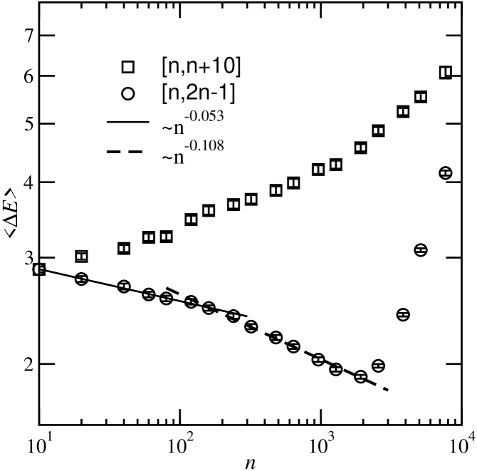
Figure 14: Average droplet energy for cross droplets ($L=160$), when the selection of the minimum droplet is restricted to a excitation size interval $[n,n+\delta(n)]$. Two cases $\delta(n)=9$ and $\delta(n)=n-1$ are shown, in the spirit of the droplet generation mechanism in Ref. berthier2003,

To compare with the results of Berthier and Young berthier2003 we have implemented a study similar to theirs for the size dependence for the cross excitations. For the largest system size $L=160$, for each realization and a given size window $[n,n+\delta(n)]$, the minimum-energy droplet was selected only among the cross excitations which lie inside the size window. Here we have studied also the case $\delta(n)=n-1$. Furthermore, instead of taking $\delta(n)=0$, we have taken $\delta(n)=9$ to improve the statistics.

In Fig. 14 the resulting average droplet energies are shown. However, the behavior we find here is totally different from that reported in Ref. berthier2003, . For the window of fixed length, the average droplet energy even goes up with $n$, while for the case $\delta(n)=n-1$, the droplet energy decreases, but for small sizes with a slower $n^{-0.53}$ power-law decrease than the $n^{-0.22}$ decrease of Ref. berthier2003, . For larger droplet sizes, a crossover can again be observed, and the data is compatible with a $n^{-0.11}$ decrease, which compares well with the $n^{-0.115}$ behavior found in Ref.berthier2003, . For very large sizes $n$, the excitations touch the boundary of the systems, where the spins are fixed. This leads to a strong increase of the droplet energy.

To understand our result for small and medium droplets, one should first note that there is an important difference between the droplets beind studied here and in Ref. berthier2003, . There, first the size was fixed, then the optimization was performed while obeying the size constraint. Here, first for each given inverted hard bond, a first optimization is performed, with a restricted search space. Then the sizes of the resulting excitations are measured and finally the minimum-energy droplet is selected among the excitations having the wanted sizes, i.e. a second optimization is performed. Note that the matching algorithm does not allow for fixing the size of a droplet in advance, so one cannot circumvent the two-stage optimization process.

We assume now that the behavior of $\Delta E$ can be understood in the following way. The distribution of excitation energies $P_{n}(\Delta E^{\star})$, obtained after the first minimization procedure, is taken as input. For each size, the final droplet is selected as minimum among a given number of excitations which we denote as $M(n)$. Hence a behavior $\Delta E\sim 1/(M(n)P_{n}(0))$ can be expected, as in the case of the first excitation discussed in the last section. We shall now test this assumption using the available data for the case $\delta(n)=n-1$.

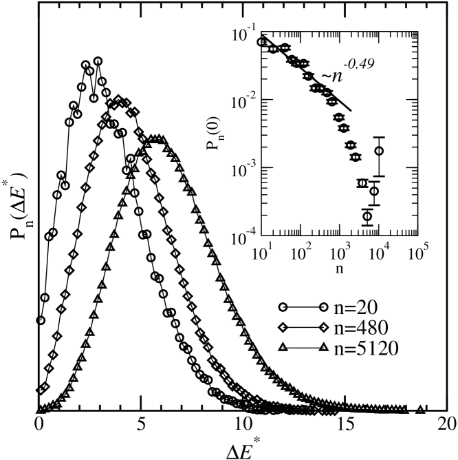
Figure 15: Distribution of energies for all cross excitations ($L=160$), restricted to a size interval $[n,n+\delta(n)]$, here $\delta(n)=n-1$. The inset shows the behavior of $P(0)$ as a function of size. The line in the inset denotes a power law $n^{-0.49}$

In Fig. 15 the distributions $P_{n}(\Delta E^{\star})$ of excitation energies are shown for different sizes $n$. Also the dependence of $P_{n}(0)$ on $n$ is shown in an inset. Due to numerical problems in determining $P_{n}(0)$, especially for small excitations, the fluctuations are quite large. If one assumes a power law decrease, the data is roughly compatible with a $n^{-0.49}$ behavior for small $n$. But, in fact, no region with a clear power-law behavior can be easily identified here.

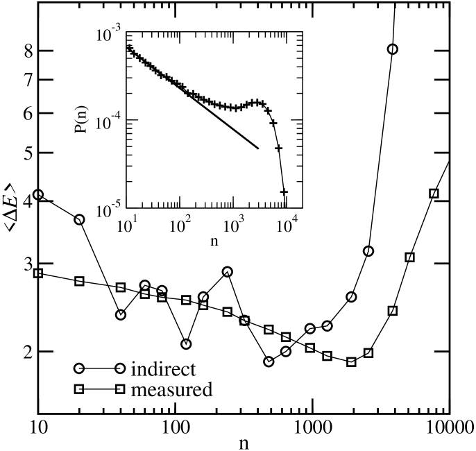
Figure 16: Average droplet energy for cross droplets ($L=160$), when the selection of the minimum droplet is restricted to a excitation size interval $[n,2n-1]$. The numerical data from Fig. 14 is repeated here (“measured”) and compared to the function $c/(M(n)P_{n}(0))$, with the scaling factor $c=2700$ (“indirect”). The inset shows the distribution of sizes of the cross excitations. $M(n)$ is obtained by integrating $P(n)$ over intervals of size $\delta(n)$.

$M(n)$ can be obtained from the distribution $P(n)$ of excitation sizes, see the inset of Fig. 16, via $M(n)\sim\int_{n}^{n+\delta(n)}P(n)dn$. In the main part of Fig. 16, $c/(M(n)P_{n}(0))$, with $c=2700$ chosen by hand. is compared to $\Delta E$. The agreement is fair, and the large fluctuations originate in the numerical problems when determining $P_{n}(0)$. One can circumvent this fluctuations for the small-size data, by using scaling arguments. From a fit to the small size range $n\in[10,100]$ one obtains $P(n)\sim n^{-0.46(2)}$. Since the selection is done in a range $O(n)$, one has $M(n)\sim n^{-0.46+1}\sim n^{0.54}$. In combination with the above result $P_{n}(0)\sim n^{-0.49}$ one obtains $\Delta E\sim 1/(M(n)P_{n}(0))=1/(n^{0.54}n^{-0.49})=n^{-0.05}$, in agreement with the direct fit of the numerical data, see Fig. 14.

For the case of fixed window size, each droplet is selected among $M(n)\sim P(n)\sim n^{-0.46}$ droplets. Hence a increase of $\Delta E$ is not surprising here. But the numerical problems due to a much smaller ($O(1)$ opposed to $O(n)$) statistics when determining $P_{n}(0)$ are too large in this case, such that a direct comparison cannot be performed.

To summarize, the two recipes to generate fixed-size droplets are different here and in the work of Berthier and Young. Hence, in general different results come out. But for the case of size fluctuations $\delta(n)=(n-1)$, the scaling behavior is the same. Since fluctuations $O(n)$ of the droplet size seem to be the most natural case, directly in the spirit of the droplet pictures by Fisher and Huse FH , it seems not surprising that in this case the results are similar. In our case it stems from a complex interplay of the selection mechanism and the behavior of the distribution $P(n)$ of excitation sizes as well as the distribution $P_{n}(\Delta E^{\star})$ of excitation energies for small energies. No direct relation to the scaling exponent $\theta$ is obvious. Furthermore, unfortunately, this still does not allow us to understand why for the $\delta(n)=O(1)$ case Berthier and Young found the same scaling behavior, but without the crossover usually seen at small to medium system sizes.

VII Summary and outlook

We have studied droplets and first excitations for two-dimensional spin glasses with Gaussian interactions. Using highly sophisticated matching algorithms, large sizes can be studied, but one is limited in the flexibility of the recipes for droplet generation.

We studied four different types of droplets/excitations and observed in general that the results depend strongly on the way droplets are generated. The single-bond droplets were very simple to generate. They do not compare with typical droplets, which are assumed to be obtained e.g. by the method of Kawashima and Aoki, because in the thermodynamic limit their energy converges to a non-zero value. The cross droplets, already introduced in Ref. droplets, , are almost equivalent to the single-spin droplets, i.e. can be considered as typical, and they show many properties expected from scaling theory. Much larger sizes than with Monte Carlo methods can be studied, hence the crossover to the $L^{\theta}$ ($\theta=-0.29$) behavior observed. Also the distribution of the droplet energies is almost as expected, except the fact the the scaling assumption does not work very close to zero energy. When studying first excitations, again much larger sizes than in previous works are possible when using the matching approach. Different results are obtained for free and fixed boundary conditions. Unfortunately, in this case the range of accessible sizes is even for the powerful algorithm used still too small to decide whether in the thermodynamic limit both cases agree and what the final scaling behavior will be. Finally, the study of fixed-volume droplets shows the limitations of the matching approach. It is not possible to use the matching algorithm to generate droplets that are really equivalent to the droplets generated by Berthier and Young. Nevertheless, it is possible to understand the scaling behavior of the droplets generated here in terms of the distributions of the excitations and their sizes. Furthermore, for the case of fluctuating volumes, which is believed to represent the typical behavior in the spirit of the DS theory, even the same scaling behavior as obtained by Berthier and Young is found.

For the single-bond and the cross droplets, their behavior seems to be clear. For the first excitations, since the matching algorithm runs in polynomial time, and because the generation of first excitations requires $O(L^{2})$ calls, the arrival of more powerful computers will resolve sooner or later the question concerning the role of boundary conditions. It would be desirable to tackle also the last open point raised by this paper: is it possible to extend or modify the matching technique, such that real fixed-size droplets can be studied? This would allow to understand their behavior better as well.