On metric structure of ultrametric spaces

Abstract

In our work we have reconsidered the old problem of diffusion at the boundary of ultrametric tree from a ”number theoretic” point of view. Namely, we use the modular functions (in particular, the Dedekind $\eta$–function) to construct the ”continuous” analog of the Cayley tree isometrically embedded in the Poincare upper half-plane. Later we work with this continuous Cayley tree as with a standard function of a complex variable. In the frameworks of our approach the results of Ogielsky and Stein on dynamics on ultrametric spaces are reproduced semi-analytically/semi-numerically. The speculation on the new ”geometrical” interpretation of replica $n\to 0$ limit is proposed.

I Introduction

Let us begin with an obvious and almost tautological statement: any regular tree has an ultrametric structure. Recall that ultrametricity of the space ${\cal H}$ implies the ”strong triangle inequality” meaning that the distances $r_{AB}$, $r_{BC}$ and $r_{AC}$ between any three points $A,B,C$ in the space ${\cal H}$ satisfy the condition $r_{AC}\leq\max\left\{r_{AB},r_{BC}\right\}$ (see, for example, rammal ). Appearing in mathematical literature in connection with $p$–adic analysis (see, for review freund ; volovich ), ultrametric spaces became very popular in physical community because of their importance for spin glasses—see, for review mezard , and references therein.

The famous replica symmetry breaking (RSB) scheme parisi is ultimately connected to the ultrametric structure of the phase space of many disordered systems possessing the spin–glass behavior. Since invention of RSB, many authors, both physicists and mathematicians, attempted to adapt the $p$–adic analysis for physical needs mainly trying to elucidate and justify the replica $n\to 0$ limit. However to our point of view the interpretation of spin–glass problems in terms of $p$–adic language does not converge well. As an exception one has to mention recent interesting contributions to that subject avet1 ; sourl ; avet2 , where the application of $p$–adic Fourier transform allows significantly simplify the solution to the problem of diffusion on ultrametric tree. One can hope that the continuation and generalization of these works would release deeper penetration of $p$–adic analysis into physics of disordered systems with ultrametric phase spaces, such as spin glasses, neural networks and disordered heteropolymers (see avet2 ; avet3 for the detailed list of corresponding references).

In what follows we shall always keep in mind the $p+1$–branching Cayley tree as an example of an ultrametric space. Despite extremely simple topological structure of a tree, one cannot operate in this space as in usual space with an Euclidean metric because the number of degrees of freedom for the $p+1$–branching Cayley tree grows exponentially with the size of a tree. For some problems, such as, for example, the branching process on Cayley trees and tree–like graphs it is not sufficient to deal only with the ”distance” measured in number of generations between two points on the graph, but it is ultimately necessary to know the absolute values of coordinates of points on the Cayley tree. The main difficulty concerns the encoding of the Cayley tree vertices. This problem becomes very cumbersome because for the tree we do not have any transparent and convenient ”coordinate system”, like a D–dimensional grid in a D–dimensional Euclidean space. One of possible ways to resolve the addressed problem consists in using the $p$–adic analysis dom1 ; dom2 . The vertices of the graph ${\cal C}$, i.e. of the $p+1$–branching Cayley tree, admit the natural parameterizations by the $p$–adic numbers what enables to develop the whole machinery like $p$–adic Fourier transform etc. This way has been exploited in papers avet1 ; sourl ; avet2 .

Another possibility, described in the present paper consists in the following. Instead of working with the ultrametric discrete graph ${\cal C}$, one can embed this graph in the metric space ${\cal H}$ preserving all ultrametric properties of ${\cal C}$. Let us mention that any image of a regular Cayley tree refers indirectly to the isometric embedding of a tree into the complex plane. Indeed, the Cayley tree is usually drawn in the picture in such a way that any new generation of vertices (counted from the root point) is smaller than the previous generation in geometric progression. Taking advantage of the isometric embedding, one can:

• naturally parameterize the vertices of the Cayley graph ${\cal C}$ by ordinary complex variable $z=x+iy$ in the complex plane $z$ without using any ingredients of a $p$–adic analysis;

• construct a continuous analog of a Cayley tree, i.e. a continuous space ${\cal H}$ with ultrametric properties borrowed from the initial Cayley tree.

The paper is organized as follows. In the section II we describe the way of isometric embedding of the regular 3–branching Cayley tree ${\cal C}$ into the complex upper half-plane $z=x+iy$ as well as we discuss the ultrametric properties of the resulting space ${\cal H}$. The problem of diffusion on the boundary of ultrametric tree ${\cal C}$ embedded into the space ${\cal H}$ is considered in the section III. The results are summarized in the conclusion, where we express also some conjectures concerning the possible geometrical interpretation of replica $n\to 0$ limit.

II Ultrametric structure of isometric Cayley trees

It is well known that any regular Cayley tree, as an exponentially growing structure, cannot be isometrically embedded in an Euclidean plane. Recall that the embedding of a Cayley tree ${\cal C}$ into the metric space is called ”isometric” if ${\cal C}$ covers that space, preserving all angles and distances. For example, the rectangular lattice isometrically covers the Euclidean plane ${\cal E}=\{x,y\}$ with the flat metric $ds^{2}=dx^{2}+dy^{2}$. In the same way the Cayley tree ${\cal C}$ isometrically covers the surface of constant negative curvature (the Lobachevsky plane) ${\cal H}$. One of possible representations of ${\cal H}$, known as a Poincaré model, is the upper half-plane ${\rm Im}\,z>0$ of the complex plane $z=x+iy$ endowed with the metric $ds^{2}=\frac{dx^{2}+dy^{2}}{y^{2}}$ of constant negative curvature.

In this Section we are aimed to construct the ”continuous” analog of the standard 3–branching Cayley tree by means of modular functions and analyse the structure of the barriers separating the neighboring valleys. Due to specific number–theoretic properties of modular functions these barriers are ultrametrically organized.

II.1 Continuous analog of isometric Cayley tree

To be precise, let us begin with the explicit description of the standard recursive construction which allows encoding of all vertices of the 3–branching Cayley tree ${\cal C}$ isometrically covering the surface of the constant negative curvature ${\cal H}=\{z|\,{\rm Im}\,z>0\}$. Recall that the 3–branching Cayley tree is the Cayley graph of the group $\Lambda$ which has the free product structure: $\Lambda\sim\mathbb{Z}_{2}\otimes\mathbb{Z}_{2}\otimes\mathbb{Z}_{2}$ (where $\mathbb{Z}_{2}$ is the cyclic group of 2nd order). The matrix representation of the generators $h_{1},h_{2},h_{3}$ of the group $\Lambda$ is well known (see, for example terras ):

$$h_{1}=\left(\begin{array}[]{cc}1&-\frac{2}{\sqrt{3}}\\ 0&-1\end{array}\right),\;h_{2}=\left(\begin{array}[]{cc}1&\frac{2}{\sqrt{3}}\\ 0&-1\end{array}\right),\;h_{3}=\left(\begin{array}[]{cc}0&\frac{1}{\sqrt{3}}\\ \sqrt{3}&0\end{array}\right)$$ (1)

For our purposes it is convenient to take a framing consisting of the composition of the standard fractional–linear transform and the complex conjugacy. Namely, denoting by $\bar{z}$ the complex conjugate of $z$, we consider the following action in ${\cal H}$:

$$\left(\begin{array}[]{cc}a&b\\ c&d\end{array}\right):\;z\to\frac{a\bar{z}+b}{c\bar{z}+d}$$ (2)

We raise the Cayley tree ${\cal C}$ in ${\cal H}$ as follows. Take the set of generators $\{h_{1},h_{2},h_{3}\}$ of the group ${\Lambda}$. Choose the point $(x_{0},iy_{0})=(0,i)$ as the root of the tree.

Any vertex in the generation $n$ from the root point of the tree ${\cal C}$ is associated with an element $\displaystyle M_{n}=\prod_{k=1}^{n}h_{\alpha_{k}}$ of the group $\Lambda$ (where $\alpha_{k}\in\{1,2,3\}$ for any $k$). All vertices are parameterized by the complex coordinates $z_{n}=M_{n}\Big{(}(-1)^{n}\,i\Big{)}$ in ${\cal H}$. For example, the coordinates of the points $z_{A}$ and $z_{B}$ in fig.1 we can get the following way. Multiply the generators $h_{i}$ along the trajectory in the backway order, i.e. from the points $z_{A}$ and $z_{B}$ to the root point $i$. Hence we arrive at

$$\begin{array}[]{l}M_{2}^{(A)}\equiv\left(\begin{array}[]{cc}a&b\\ c&d\end{array}\right)=h_{3}\,h_{2}=\left(\begin{array}[]{cc}0&\frac{1}{\sqrt{3}}\\ \sqrt{3}&0\end{array}\right)\left(\begin{array}[]{cc}1&\frac{2}{\sqrt{3}}\\ 0&-1\end{array}\right)=\left(\begin{array}[]{cc}0&-\frac{1}{\sqrt{3}}\\ \sqrt{3}&2\end{array}\right)\vskip 6.0pt plus 2.0pt minus 2.0pt\\ M_{3}^{(B)}\equiv\left(\begin{array}[]{cc}a&b\\ c&d\end{array}\right)=h_{3}\,h_{2}\,h_{3}=\left(\begin{array}[]{cc}0&\frac{1}{\sqrt{3}}\\ \sqrt{3}&0\end{array}\right)\left(\begin{array}[]{cc}1&\frac{2}{\sqrt{3}}\\ 0&-1\end{array}\right)\left(\begin{array}[]{cc}0&\frac{1}{\sqrt{3}}\\ \sqrt{3}&0\end{array}\right)=\left(\begin{array}[]{cc}-1&0\\ 2\sqrt{3}&1\end{array}\right)\end{array}$$

Using (2) and the matrices $M_{2}^{(A)}$ and $M_{3}^{(B)}$, we get

$$\begin{array}[]{l}\displaystyle z_{A}=\frac{0\times i-\frac{1}{\sqrt{3}}}{\sqrt{3}\times i+2}=-\frac{2}{7\sqrt{3}}+\frac{i}{7}\vskip 6.0pt plus 2.0pt minus 2.0pt\\ \displaystyle z_{B}=\frac{(-1)\times(-i)+0}{2\sqrt{3}\times(-i)+1}=-\frac{2\sqrt{3}}{13}+\frac{i}{13}\end{array}$$

To establish the connection with the forthcoming constructions, we shall make the simple linear transform of $z:z\to\frac{\sqrt{3}}{2}z+\frac{1}{2}$. The coordinates of the points $A$ and $B$ are shown in Fig.1 after such transform.

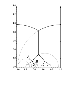
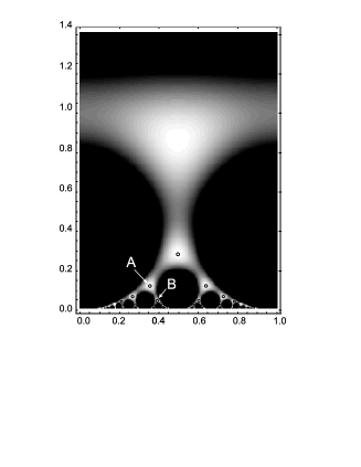
Figure 1: Left: 3–branching Cayley tree isometrically embedded in Poincaré hyperbolic upper half-plane ${\cal H}$. Right: Density plot of the function $f(z)$ (see the text) in the rectangle $\{0\leq{\rm Re}\,z\leq 1,\;0.01\leq{\rm Im}\,z\leq 1.4\}$.

However such recursive construction has, to our point of view, the crucial lack: one cannot automatically encode all vertices of the tree introducing a sort of a ”coordinate system” as, say, in the Euclidean plane. Actually, we know that any vertex of a rectangular grid in the Euclidean plane has the coordinates $(a\,m,\;b\,n)$, where $\{m,n\}\in Z$ and $(a,b)$ are the length and the width of the elementary cell of the lattice. Our desire is to construct somewhat similar for homogeneous trees. To be more specific, we are aimed to find an analytic function $f(z)$ defined in ${\rm Im}\,z>0$ whose all zeros give all coordinates of the vertices of the 3–branching homogeneous Cayley tree ${\cal C}$ isometrically embedded into ${\cal H}(z|{\rm Im}\,z>0)$. In the rest of this Section we describe the construction of the corresponding function $f(z|{\rm Im}\,z>0)$ and discuss its properties in connection with the geometry of ultrametric spaces. The forthcoming construction is based on the properties of the Dedekind $\eta$–function. Recall the standard definition of the $\eta(z)$–function (see, for instance chand ):

$$\eta(z)=e^{\pi iz/12}\prod_{k=0}^{\infty}(1-e^{2\pi ikz});\qquad{\rm Im}\,z>0$$ (3)

It is well known chand that the Dedekind $\eta$–function is connected to the elliptic Jacobi $\vartheta$–functions by the following relation:

$$\vartheta_{1}^{\prime}(0,e^{\pi iz})=\eta^{3}(z)$$ (4)

where

$$\vartheta_{1}^{\prime}(0,e^{\pi iz})\equiv\frac{d\vartheta_{1}(u,e^{\pi iz})}{du}\bigg{|}_{u=0}=2e^{\pi iz/4}\sum_{n=0}^{\infty}(-1)^{n}(2n+1)e^{\pi in(n+1)z}$$ (5)

Now we are in position to formulate the central assertion of the paper. Define the function $f(z)$ as follows:

$$f(z)=C^{-1}\,|\eta(z)|\,({\rm Im}\,z)^{1/4}$$ (6)

where $C$ is the normalization constant,

$$C=\left|\eta\left(\frac{1}{2}+i\frac{\sqrt{3}}{2}\right)\right|\,\left(\frac{\sqrt{3}}{2}\right)^{1/4}=0.77230184...$$ (7)

The normalization constant $C$ is chosen to set the maximal value of the function $f(z)$ to 1: $0<f(z)\leq 1$ for any $z$ in the upper half-plane ${\rm Im}\,z>0$. It can be proved that the function $f(z)$ has the following remarkable properties:

1. The function $f(z)-1$ has zeros at the points $z_{\rm cen}$ (and only at these points) – the centers of zero–angled triangles tesselating the Poincaré hyperbolic upper half-plane ${\cal H}(z|{\rm Im}\,z>0)$;

2. The function $f(z)$ has local maxima at all the points $z_{\rm cen}$ and only at these points.

All the solutions of the equation $f(z)-1=0$ define all the coordinates of the 3–branching Cayley tree isometrically embedded into the upper half-plane ${\cal H}(z|{\rm Im}\,z>0)$. The corresponding density plot of the function $f(z)$ in the region $\{0\leq{\rm Re}\,z\leq 1,\;0.04\leq{\rm Im}\,z\leq 1.4\}$ is shown in fig.2. It is noteworthy that the function $Z(z)=\left[C\,f(z)\right]^{-2}$ is the partition function of a free bosonic field on a torus franc . The function $Z(z)$ has been extensively studied in the conformal field theory. In particular it can be easily checked that the function $Z(z)$ is invariant with respect to the action of the modular group $PSL(2,\mathbb{Z})$, namely:

$$\left\{\begin{array}[]{l}Z(z)=Z(z+1)\vskip 6.0pt plus 2.0pt minus 2.0pt\\ \displaystyle Z(z)=Z\left(-\frac{1}{z}\right)\end{array}\right.$$ (8)

Later on we shall address to these self–dual properties. The proof of our assertion (6) implies the check that the function $f(z)$ is invariant with respect to the conformal transform $z^{(1)}(z)$ of the Poincaré half-plane to itself

$$z^{(1)}(z)=\frac{z-z_{0}}{z\bar{z}_{0}-1}$$ (9)

where $z_{0}$ is the coordinate of any center of zero–angled triangle in the hyperbolic Poincaré upper half–plane obtained by successive transformations from the initial one. Hence, it is necessary and sufficient to show that the values of the function $f(z)$ at nearest centers of circular triangles are equal and reach the maximal value 1:

$$f\left(z=\frac{1}{2}+i\frac{\sqrt{3}}{2}\right)=f\left(z=\pm 1+\frac{1}{2}+i\frac{\sqrt{3}}{2}\right)=f\left(z=\frac{1}{2}+i\frac{\sqrt{3}}{6}\right)=1$$ (10)

Then taking $z_{0}=\left\{\left(\frac{3}{2}+i\frac{\sqrt{3}}{2}\right);\left(-\frac{1}{2}+i\frac{\sqrt{3}}{2}\right);\left(\frac{1}{2}+i\frac{\sqrt{3}}{6}\right)\right\}$ and performing the conformal transform (9) we move the centers of the first generation of zero–angled triangles to the new centers (second generation) located at $z^{(1)}$. Now we can repeat recursively the construction, i.e. find the new coordinates of the centers of the third generation of zero–angled triangles, $z^{(2)}(z^{(1)})$, and compute the function $f(z)$ at these points, then we perform the conformal transform $z^{(3)}(z^{(2)})$ and so on… Let us use now the following well–known properties of Jacobi elliptic $\vartheta$–functions chand

$$\eta\left(\frac{pz+r}{qz+s}\right)=\omega\sqrt{rz+s}\;\eta(z)$$ (11)

where ${\rm Im}\,z>0$, $\{p,q,r,s\}\in Z$; $ps-qr=1$ and $\omega$ is some 24–power root of unity, which depends on the coefficients $p,q,r,s$ but does not depend on $z$. Using (11) we can write:

$$\left\{\begin{array}[]{ll}\eta(z+k)=\eta(z);&\quad k=\pm 1,\pm 2,\pm 3,...\vskip 6.0pt plus 2.0pt minus 2.0pt\\ \eta\left(\frac{1}{2}+\frac{i}{2\sqrt{\lambda}}\right)\lambda^{-1/4}=\eta\left(\frac{1}{2}+\frac{i\sqrt{\lambda}}{2}\right);&\quad\lambda>0\end{array}\right.$$ (12)

Now we can easily check the relations (10). In turn, (8) can be regarded as a particular case of eq.(11). The fact that the function $f(z)$ has local maxima at the points $z_{\rm cen}$ can be verified straightforwardly by differentiating $f(z)$ with respect to $z$ at the points $z_{\rm cen}$. The 3D relief of the function $f(z)$ is shown in figure 2. The tree–like structure of hills separated by the valleys is clearly seen.

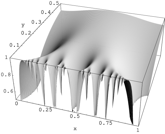
Figure 2: Relief of the function $f(z)$ in the rectangle $\{0\leq{\rm Re}\,z\leq 1,\;0.04\leq{\rm Im}\,z\leq 1.4\}$.

Let us note the important duality relation for the Dedekind function which establishes the mapping $y\leftrightarrow\frac{1}{y}$ (where $y={\rm Im}\,z$; $y>0$). For all $\{p,q,r,s\}\in Z$ such that $ps-qr=1$ the following equation is satisfied:

$$\left|\eta\left(\left\{\frac{p}{q}\right\}+i\,y\right)\right|=\left|\eta\left(\left\{\frac{s}{q}\right\}+\frac{i}{q^{2}\,y}\right)\right|\;\frac{1}{\sqrt{q\,y}}$$ (13)

where by $\left\{\frac{p}{q}\right\}$ and $\left\{\frac{s}{q}\right\}$ we denote the fractional parts of the corresponding quotients. The relation (13) shall be used in the forthcoming sections for practical purposes of numerical computations. In the next chapter we discuss the ultrametric organization of corresponding barriers. We regard the 3D relief constructed on the basis of the function $f(z)$ (see fig.2) as the continuous analog of the Cayley tree isometrically embedded in ${\cal H}(z|{\rm Im}\,z>0)$.

II.2 Ultrametric structure of barriers in the standard RSB scheme and in the tree–like metric space

The replica symmetric breaking (RSB) scheme parisi has appeared in the spin–glass theory as a self–consistent approach free of many lacks of the replica symmetric consideration. Later on it has been realized that the RSB–structure naturally appears in the problem of diffusion on the boundary of the Cayley tree os ; bachas , where the neighboring sites are separated by the barriers hierarchically organized according their ultrametric distances on the Cayley tree. For example the neighboring points $A,B$ and $B,C$ at the boundary of the 3–branching Cayley tree—see fig.3—are separated by the barriers depending on the ultrametric distance between points $A,B$ and $B,C$ on the tree.

Recall that two points, say, $B$ and $C$ in fig.3 are separated by the potential barrier depending on the number of the Cayley tree generations from the points $B$ and $C$ up to their common ”parent branch”. Let us label the states at the $L$’s generation of the 3–branching Cayley tree by the integer number $k$ ($1\leq k\leq 2^{L}$). If we represent $k$ by the binary sequence, then the ultrametric distance between points $B$ and $C$ shall coincide with the highest distinct rank in the binary writing of $k_{B}=4$ and $k_{C}=5$.

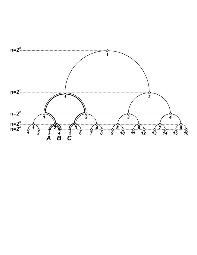
Figure 3: The 3–branching Cayley tree. The ultrametric distance between points $A,B$ and $B,C$ are shown by bold lines; $n$ is the number of states in each generation of the tree, the maximal number of generations $L=4$.

Denote by $q_{m}$ the Boltzmann weights at the boundary of 3-branching Cayley associated to the barriers of ultrametric height $m$. All the barriers can be encoded in the $2^{L}\times 2^{L}$ RSB matrix ${\bf Q}(q_{0},q_{1},...,q_{L})$ having the structure shown in eq.(14) for $L=3$. Keeping in mind the connection to the spin glasses, the total number of states $2^{L}$ is associated to the total number of replicas, $n$, in the standard RSB scheme.

$${\bf Q}=\begin{array}[]{|c|c|}\hline\cr\begin{array}[]{cc|cc}q_{0}&q_{1}&q_{2}&q_{2}\\ q_{1}&q_{0}&q_{2}&q_{2}\\ \hline\cr q_{2}&q_{2}&q_{0}&q_{1}\\ q_{2}&q_{2}&q_{1}&q_{0}\end{array}&\begin{array}[]{cccc}q_{3}&q_{3}&q_{3}&q_{3}\\ q_{3}&q_{3}&q_{3}&q_{3}\\ q_{3}&q_{3}&q_{3}&q_{3}\\ q_{3}&q_{3}&q_{3}&q_{3}\end{array}\\ \hline\cr\begin{array}[]{cccc}q_{3}&q_{3}&q_{3}&q_{3}\\ q_{3}&q_{3}&q_{3}&q_{3}\\ q_{3}&q_{3}&q_{3}&q_{3}\\ q_{3}&q_{3}&q_{3}&q_{3}\end{array}&\begin{array}[]{cc|cc}q_{0}&q_{1}&q_{2}&q_{2}\\ q_{1}&q_{0}&q_{2}&q_{2}\\ \hline\cr q_{2}&q_{2}&q_{0}&q_{1}\\ q_{2}&q_{2}&q_{1}&q_{0}\\ \end{array}\\ \hline\cr\end{array}$$ (14)

The values $p_{m}=\frac{1}{n}q_{m}$ ($m=1,...,L$) define the jumping probabilities from some vertex $k_{1}$ to another vertex $k_{2}$ at the boundary of 3-branching Cayley tree separated by the barrier of ultrametric height $m$, while the value $p_{0}$ is assigned for the probabilities to stay in a given vertex. In each line of the matrix ${\bf Q}$ the sum of probabilities is equal to 1. In most physically important situations the Boltzmann weights $q_{m}$ depend on $m$ either exponentially or polynomially:

$$q_{m}=\left\{\begin{array}[]{l}{\rm const}\;m^{\alpha}\\ {\rm const}\;e^{-\beta\,m}\end{array}\right.$$ (15)

Later on we pay attention only to the exponential dependence of $q_{m}$ on $m$, i.e. to the case when $q_{m}={\rm const}\;e^{-\beta\,m}$ (where $\beta$ stands for the inverse temperature). The probability $p_{0}$ to stay in a given vertex can be explicitly computed from the conservation condition $\sum_{m=0}^{n}P_{m}=1$ and for $q_{m}={\rm const}\;e^{-\beta\,m}$ it reads:

$$p_{0}=1-\frac{1}{n}\sum_{j=1}^{L}2^{j}\,e^{-\beta\,j}=1-\frac{2(1-2^{L}\,e^{-\beta\,L})}{n(2-e^{\beta})}$$ (16)

In order to understand the connection between the ultrametric structure of the barriers in case of 3–branching Cayley tree and its continuous analog isometrically embedded in ${\cal H}(z|{\rm Im}\,z>0)$, let us begin with the following observation. We can consider the function $v(x|y)=-\ln f(x|y)$ (where $x={\rm Re}\,z$) as the potential relief at the boundary of the Cayley tree cut at the distance $y={\rm Im}\,z$ from the real axis. The typical shapes of the function $v(x|y)$ for few fixed values $y=0.04,\,0.008,\,0.0016$ are shown in fig.4. This picture clearly demonstrates the ultrametric organization of the barriers separating the valleys.

Figure 4: Typical shape of the function $v(x|y)=-\ln f(x)$ for few values $y=0.04,\,0.008,\,0.0016$.

As one can see in fig.4, the distance from the real axis, $y$, characterizes the number of the Cayley tree generation: as closer is the value $y$ to the real axis, as more new generations of barriers appear (and as higher are the barriers). The relation of the system of barriers shown in fig.4 with the structure of RSB matrix (14) becomes now very straightforward. The barriers of smallest scale correspond to the values $q_{1}$ in the matrix ${\bf Q}(q_{0},q_{1},...,q_{L})$, the barriers of the next scale correspond to $q_{2}$ etc… Hence the distance $y$ might be considered as the parameter controlling the size of the RSB matrix: as $y\to 0$ the size of ${\bf Q}$ tends to infinity. Thus, one can conjecture that the number of the replicas, $n$, is the function of $y$.

This relation shall be discussed in more details at length of the next section. The function $v(x)=-\ln f(x)$, defined on the interval $0<x<1$, has the properties borrowed from the structure of the underlying modular group $PSL(2,\mathbb{Z})$ acting in the half–plane ${\cal H}(z|y>0)$ magnus ; beardon . In particular:

• The local maxima of the function $v(x)$ are located at the rational points;

• The highest barrier on a given interval $\Delta x=[x_{1},x_{2}]$ is located at a rational point $\frac{p}{q}$ with the lowest denominator $q$. On a given interval $\Delta x=[x_{1},x_{2}]$ there is only one such point. The locations of the barriers with the consecutive heights on the interval $\Delta x$ are organized according to the group operation:

  $$\frac{p_{1}}{q_{1}}\oplus\frac{p_{2}}{q_{2}}=\frac{p_{1}+p_{2}}{q_{1}+q_{2}}$$ (17)

The figures 4 clarifies this statement. The highest barriers on the interval $0\leq x\leq 1$ are located at the points $x_{0}=0$ and $x_{1}=1$. Rewriting $0$ and $1$ correspondingly as $\frac{0}{1}$ and $\frac{1}{1}$ we can find the point $x_{2}$ of location of the barrier with the next maximal hight. Namely, $x_{2}=\frac{0}{1}\oplus\frac{1}{1}=\frac{0+1}{1+1}=\frac{1}{2}$. Continuing this construction we arrive at the hierarchical structure of barriers located at rational points organized in the Farey sequence. According to our construction this should replace the standard RSB scheme. The corresponding ”modular” (MRSB) matrix shall be constructed in the next section.

II.3 Explicit organization of barriers on the basis of Dedekind function

The said above gives the idea of the construction. However to establish the precise connection between the standard RSB scheme and the ”number–theoretic” MRSB scheme, we should construct the MRSB scheme with exponential organization of the Boltzmann weights—as in RSB. Recall that the ultrametric distance between two points $A$ and $B$ on the Cayley graph is equal to one half of the number of steps of the shortest path connecting these points. For example, the ultrametric distances $r_{AB}$ (between points $A$ and $B$) and $r_{AC}$ (between points $A$ and $C$) in fig.3 are as follows: $r_{AB}=1$ and $r_{AC}=3$. It is clearly seen that the points $A$ and $B$ (as well as the points $B$ and $C$) are separated by the barrier located at the point $x_{1}=\frac{1}{3}$, while the points $A$ and $B$ are separated by the barrier located at the point $x_{2}=\frac{2}{7}$. According to the last of eqs.(15), the height $U_{m}$ of the barrier between two points separated by the ultrametric distance $m$ in the standard RSB scheme reads

$$U_{m}^{RSB}\equiv-\ln q_{m}=\beta\,m$$ (18)

The dependence of Boltzmann weights on the ultrametric distance in the MRSB scheme should also satisfy (18). This implies that the heights $U_{MRSB}$ of the MRSB–barriers should linearly depend on the ultrametric distance between two vertices of the Cayley tree. To adjust the heights of the barriers in MRSB and RSB schemes some auxiliary work has to be done. The corresponding construction is described in the rest of this section. Begin with the standard RSB tree and distribute barriers separating all $2^{L}$ boundary points of the Cayley tree in the generation $L$ equidistantly in the unit interval $[0,1]$. For example, for $L=1$ there are 2 vertices of the Cayley tree separated by a single barrier located at the point $x_{1}=\frac{1}{2}$. The barriers of the second generation $L=2$ are placed at the points $x_{2}^{(1)}=\frac{1}{4}$ and $x_{2}^{(2)}=\frac{3}{4}$. For $L=3$ we have $x_{3}^{(1)}=\frac{1}{8}$, $x_{3}^{(2)}=\frac{3}{8}$, $x_{3}^{(3)}=\frac{5}{8}$, $x_{3}^{(3)}=\frac{7}{8}$ etc. The points $x_{L}^{(j)}=\frac{j}{2^{L}}$ (where $j$ is odd and $1<j<2^{L}$) cover uniformly the unit interval $[0,1]$. Let us normalize the barrier heights as follows. In the finite Cayley tree of $L$ generations there are $2^{L-1}$ smallest barriers; all of them have equal heights. Demand these barriers be of height $U(L)=\frac{1}{L}$. Then the averaged barriers in some intermediate generation $m$ ($1\leq m\leq L$) have the height

$$U(m,L)=\frac{L-m+1}{L}\equiv 1-\frac{m-1}{L}$$ (19)

Hence, in the first generation $m=1$ the height of a single barrier located at the point $x_{1}=\frac{1}{2}$ is normalized by 1: $U(m=1,L)=1$. This sets our normalization condition. Let us note that the choice of the normalization of the barriers might be considered as the renormalization of the inverse temperature $\beta\to\tilde{\beta}L$ (see (18)). The ”physical” sense of such renormalization consists in the following. When the number of Cayley tree generations $L$ is increased, the corresponding landscape acquires more and more small–scale details without changing the height of the maximal barrier, which is always normalized by 1.

Now we proceed in the similar way with the continuous MRSB–structure. Recall that the logarithm of the Dedekind function has maxima at the rational points $x=\frac{p}{q}$. The set of these points $\{x_{i}\}$ can be generated recursively as it has been explained above in connection with eq.(17). We start with two ”parent” points $0=\frac{0}{1}$ and $1=\frac{1}{1}$ of zero’s generation. On the first step we generate a barrier at the point $\frac{1}{r2}=\frac{0+1}{1+1}$; on the second step we generate two barriers at the points $\frac{1}{3}=\frac{0+1}{1+2}$ and $\frac{2}{3}=\frac{1+1}{2+1}$ and so on… The number of recursive steps necessary to arrive at a barrier located at a specific point $x=\frac{p}{q}$ we shall call the generation in which this barrier has appeared for the first time.

Let us fix the maximal generation $L$. Define $\{x_{i}\}(m)$ the set of points in the generation $m\leq L$ at which the barriers are located. There are $2^{m-1}$ such points. For example, $\{x_{i}\}(m=1)=\{\frac{1}{2}\}$, $\{x_{i}\}(m=2)=\{\frac{1}{3},\frac{2}{3}\}$, $\{x_{i}\}(m=3)=\{\frac{1}{4},\frac{2}{5},\frac{3}{5},\frac{3}{4}\}$ and so on. Now we need to express the heights $U_{MRSB}(x_{i},m,y)$ of the barriers up to the generation $m\leq L$ via the Dedekind function $\eta(x_{i},y)$. Take the logarithm of the normalized Dedekind function

$$h(x,y)=-\ln f(x,y)$$ (20)

as the possible basis for such construction (the function $f(x,y)$ is defined in (6)). Our choice is justified by the fact that this function has maxima at the points $\{x_{i}\}(m)$ and demonstrates the ultrametric behavior. Starting from $m\geq 3$, the values of the function $h(x_{i},m,y)$ at the points of maxima $\{x_{i}\}(m)$ become not equal. In fig.5a we have plotted the minimal $h_{min}(m,y)={\rm min}(h(x_{i},m,y))$, the average $h_{avr}(m,y)=\left<h(x_{i},m,y)\right>$ and the maximal $h_{max}(m,y)={\rm max}(h(x_{i},m,y))$ barrier heights in each of three generations $m=4,6,8$. The brackets $\left<\dots\right>$ denote averaging over all barriers in the generation $m$. The function $0.001\,y^{-1}$ is plotted for comparison in the same figure.

Figure 5: a) Minimal $h_{min}(y)$, average $h_{avr}(y)$ and maximal $h_{max}(y)$ barriers for $m=4,6,8$; b) The function $h_{avr}(y)$ for $m=1,...,10$.

The figure 5a allows us to conclude that $h(m,y)\sim y^{-1}$ for fixed $m$. More detailed information about the function $h_{avr}(m,y)=\left<-\ln(\eta(x_{i},y))\right>$ can be extracted from the fig.5b, which is similar to the fig.5a but is extended up to $m\in[1,10]$. The data shown in fig.5b is approximated by the natural fit

$$h_{avr}=a_{m}y^{b_{m}}$$

for all points such that $h_{avr}>10$. The results of our approximation are shown in the Table 1a as well as are drawn in fig.5b by lines.

$~{}m$	$~{}a_{m}$	$~{}b_{m}$
1	0.0594(8)	-1.008(2)
2	0.0263(4)	-1.008(1)
3	0.0118(2)	-1.011(1)
4	0.0053(1)	-1.014(2)
5	000230(7)	-1.021(3)
6	0.00084(7)	-1.04(1)
7	0.00031(4)	-1.06(1)
8	0.000118(17)	-1.08(6)
9	0000040(7)	-1.102(1)
10	0000012(3)	-1.14(2)

$~{}y^{*}$	$~{}c(y^{*})$
$~{}5.12\times 10^{-5}$	0.820(11)
$~{}2.56\times 10^{-5}$	0.8057(99)
$~{}1.28\times 10^{-5}$	0.7944(86)
$~{}6.4\times 10^{-6}$	0.7718(29)
$~{}3.2\times 10^{-6}$	0.7623(22)
$~{}1.6\times 10^{-6}$	0.7579(27)
$~{}8\times 10^{-7}$	0.7556(30)
$~{}4\times 10^{-7}$	0.7544(32)
$~{}2\times 10^{-7}$	0.7538(37)
$~{}1\times 10^{-7}$	0.7535(34)

Table 1: a) Numerical results of the fit $h_{avr}=a_{m}y^{b_{m}}$; b) Dependence of the parameter $c(y)$ on $y=y^{*}$ up to $L=10$ generations—see eq.25.

We have plotted the coefficient $a_{m}$ as a function of $m$ in fig.6a. The approximation $a_{m}\simeq 0.144(8)\,e^{-0.847(18)\,m}$ is shown in the same figure by dashed line. Hence, we expect the following relation $h(m,y)\simeq 0.144(8)\,e^{-0.847(18)\,m}\,y^{-1}$.

Figure 6: a) Approximation of the coefficient $a_{m}$; b) Ultrametric barriers $U_{MRSB}(m,y)=\frac{1}{c(y)\,L}\ln\frac{h(m,y))}{h(1,y)}$.

The analysis of the numerical data for the averaged logarithm of the Dedekind function allows us to conjecture the general ansatz

$$h_{avr}(m,y)\equiv\left<-\ln f(x_{i},y)\right>=d(y)\,e^{-c(y)\,m}\,y^{-1}$$ (21)

This equation establishes the functional dependence of the average height $h_{avr}$ on the generation $m$ ($m=1,2,...$) for fixed $y$. Recall that the generation $m$ is defined as the minimal number of recursive steps necessary to arrive at a barrier located at a specific point $x_{i}=\frac{p}{q}$. Let us fix now the maximal generation $L$. Our desire is to obtain the normalized barrier for MRSB scheme like it has been done for RSB (see eq.(19)). Taking into account that (21) is valid for any $m\geq 1$, we may extract $m$ from (21) and write it as follows

$$m=1+\frac{1}{c(y)}\ln\frac{h_{avr}(m,y)}{h_{avr}(m=1,y)}$$ (22)

Substituting (22) into (19) we get the following formal expression for the height of the barriers in the MRSB scheme

$$U_{MRSB}(x_{m},y,L)\equiv 1-\frac{m-1}{L}=1+\frac{1}{c(y)\,L}\ln\frac{h_{avr}(m,y)}{h_{avr}(1,y)}$$ (23)

Now we should explain how it is possible to use the formal equation (23) in practical computations. Let us fix the maximal generation $L$ and define the value $y^{*}$ from the equation

$$h_{avr}(y^{*},L)=1$$ (24)

The value $y^{*}$ has the following sense. For all $y<y^{*}$ the value $h_{avr}(m,y)$ does not depend on $m$ ($m\leq L$) because all barriers in the generation $m$ are already presented and hence the average hight $h_{avr}$ can not be changed for any $y<y^{*}$. Therefore we can postulate, that for all $y<y^{*}$ the height of the barrier is described by the function

$$U_{MRSB}(x_{i})=1+\frac{1}{c(y^{*})\,L}\ln\frac{\ln f\left(x_{i},y^{*}\right)}{\ln f\left(\frac{1}{2},y^{*}\right)}$$ (25)

where $x_{i}$ is the rational point of the barrier location and we have used (20). Special attention deserves the discussion of the dependence $c(y^{*})$. As it is shown in the Table 1b, for sufficiently small $y^{*}$ the value of $c$ tends to the constant value. Thus the function $U_{MRSB}(x_{i})$ defines the heights of ultrametric barriers in MRSB scheme fully consistent with the heights of the RSB–barriers for the Cayley tree. It should be noted that for intermediate values of $y$ some barriers of large generations are negative due to the cut (24), however having $m$, we can always find $y^{*}$ such that all barriers are positive. For example, for $y\leq y^{*}=10^{-6}$ all barriers up to $m=10$ generations are positive.

Figure 7: Ultrametric barriers $U_{MRSB}(x_{i})$ at the rational points $x_{i}$ for $y=10^{-6}$

Our tedious but simple construction is clearly explained in the figure 7, where we have plotted the heights of barriers $U_{MRSB}(x_{i})$ at the rational points $x_{i}$ up to the generation $L=10$ for $y^{*}=10^{-6}$. Once the maximal generation $L$ is fixed and all barriers for all generations (up to the maximal one) are shown in the picture, then this picture is unchanged for all $y$ such that $y<y^{*}$. According to our definition, these barriers are normalized in such a way that the height of the largest barrier is equal to $1$. The averaged height of the barriers of second (third, forth, etc…) generation is equal to $0.9$ ($0.8$, $0.7$, etc…) – compare to (19). Let us repeat that in fig.7 we have displayed the barriers corresponding to generations $m$ up to $m=L$. We can easily relax this condition and work with the set of all possible barriers up to some fixed minimal value $y_{min}$ without paying attention how many generations are counted.

II.4 Description of dynamical models

Our aim is to investigate numerically the probability distribution of a random walk on the boundary of an ultrametric space. This problem has been a subject of the original work os where the dynamics in the ultrametric space was considered in the frameworks of the discrete model of jumps on the boundary of 3–branching Cayley tree. The first application of $p$–adic analysis for the computation of the probability distribution of the diffusion at the boundary of the ultrametric tree has been successfully realized in avet1 .

Below we reconsider the diffusion problem in the continuous metric space, where the ultrametric organization of the barriers is due to the modular structure of the Dedekind function. The advantages of such consideration we shall discuss in the Conclusion. Let us specify the models under consideration.

II.4.1 I. The standard RSB model

In this model we consider the random jumps at the boundary of 3–branching Cayley tree—see fig.3. The transition probabilities between the Cayley tree vertices are encoded in the matrix (14). As explained above, we fix the total number of generations $L$ and set the highest barrier (in the first generation) always equal to 1. Then the heights of the barriers of generation $m$ are given by (19), while the height of the smallest barriers in the generation $L$ is equal to $\frac{1}{L}$. Increasing the number of generations $L$, we increase the resolution of our model without changing the value of the maximal barrier. We use this problem of diffusion on the boundary of the standard 3–branching Cayley tree as a testing area for diffusion in the continuous tree–like ultrametric space.

Let $P_{N}(k,k_{0})$ be the partition function of the random walk starting at the point $k_{0}$ and ending after $N$ steps at the point $k$, where $k$ labels the vertices of the $k$’s generation of the Cayley tree and both points $k_{0}$ and $k$ belong to the $m$’s generation of the tree. The corresponding diffusion is governed by the recursion relation

$$\left\{\begin{array}[]{l}\displaystyle P^{RSB}_{N+1}(k)=\sum_{k^{\prime}=0}^{2^{L}-1}Q^{RSB}(k,k^{\prime})P^{RSB}_{N}(k^{\prime})\\ \displaystyle P^{RSB}_{N=0}(k)=\delta_{k,k_{0}}\end{array}\right.$$ (26)

where $Q^{RSB}(k,k^{\prime})$ is the $2^{L}\times 2^{L}$ matrix whose elements are the Boltzmann weights associated with jumps from some point $k_{1}$ to the point $k_{2}$ ($\{k_{1},k_{2}\}\in[1,2^{L}]$) at the boundary of 3–branching Cayley tree cut at the generation $L$. In order to take into account the ultrametricity of the Cayley tree, the matrix $Q^{RSB}(k,k^{\prime})$ should have the RSB structure and hence should coincide with the matrix ${\bf Q}$ in (14).

II.4.2 II. The quasi-continuous MRSB model

This model is defined as follows. We fix the maximal generation $L$ and consider the heights of the potential $U^{MRSB}$ (see (25)) corresponding to generations less or equal $L$. For example, in fig.8a we have plotted $15=2^{L}-1=n$ barriers up to $L=4$ generation. The rational points $x_{i}$ split the interval $[0,1]$ into 16 subintervals $[x_{i-1},x_{i}],\;i=1,2,...,15$ (including the subintervals $[0,x_{1}]$ and $[x_{15},1]$). The random walker can jump form one interval to any other. Let us enumerate the intervals by the variable $k=1,2,3,...,16$. So, $k=1$ denotes the interval $[0,x_{1}]$, $k=2$ is the interval $[x_{1},x_{2}]$, etc. Let $U_{MRSB}(k,k^{\prime})$ be the maximal barrier between the intervals $k$ and $k^{\prime}$ defined by (25). By construction $U^{MRSB}(k,k)=0$. According to our rules if $x\in[x_{k-1},x_{k}]$ and $x^{\prime}\in[x_{k^{\prime}-1},x_{k^{\prime}}]$ then $U^{MRSB}(x,x^{\prime})=U^{MRSB}(k,k^{\prime})$. Thus we can write the recursive relation for the continuous distribution function $W_{N}(x)$. This function is defined for $x\in{\mathbb{R}},\;(0\leq x\leq 1)$, where $N$ enumerates the time moments. We claim for this quasi-continuous MRSB case the following form of the master equation which should replace eq.(26).

$$\left\{\begin{array}[]{l}\displaystyle W_{N+1}(x)=\int_{0}^{1}dx^{\prime}\,e^{\displaystyle-\beta U_{MRSB}(x,x^{\prime})}\;W_{N}(x^{\prime})\\ \displaystyle W_{N=0}(x)=\delta_{x,x_{0}}\end{array}\right.$$ (27)

Figure 8: a) Location of barriers up to 4 generations: a) Model I: the values $v_{i}$ correspond to the intervals between maxima; b) Model II: the values $v_{i}$ correspond to the discrete points.

We can transform (27) making it more similar to (26). Namely, define $P^{MRSB}_{N}(k)$ – the probability that the walker belongs to the $k$-th interval on the $N$-th jump (time step)

$$P^{MRSB}_{N}(k)=\int_{x_{k-1}}^{x_{k}}W_{N}(x)dx$$ (28)

The normalization of the probability defines the sum over all intervals $\sum_{k=1}^{n}P^{MRSB}_{N}(k)=\int_{0}^{1}W_{N}(x)dx=1$. Integrating (27) over the interval $[0,1]$ and replacing the integrals over $dx$ and $dx^{\prime}$ by sums over $k$ and $k^{\prime}$, we get

$$\begin{array}[]{lll}\displaystyle\sum_{k=1}^{n}P^{MRSB}_{N+1}(k)&=&\displaystyle\int_{0}^{1}W_{N+1}(x)dx=\int_{0}^{1}\int_{0}^{1}\,e^{\displaystyle-\beta U_{MRSB}(x,x^{\prime})}\;W_{N}(x^{\prime})dx^{\prime}dx\\ &=&\displaystyle\sum_{k=1}^{n}\sum_{k^{\prime}=1}^{n}\int_{x_{k-1}}^{x_{k}}\int_{x^{\prime}_{k^{\prime}-1}}^{x^{\prime}_{k^{\prime}}}e^{\displaystyle-\beta U_{MRSB}(x,x^{\prime})}W^{MRSB}_{N}(k^{\prime})dx^{\prime}dx\\ &=&\displaystyle\sum_{k=1}^{n}\sum_{k^{\prime}=1}^{n}l_{k}e^{\displaystyle-\beta U_{MRSB}(k,k^{\prime})}P^{MRSB}_{k^{\prime}}\end{array}$$ (29)

where $l_{k}$ is the length of the $k$-th interval $l_{k}=\int_{x_{k-1}}^{x_{k}}dx=x_{k}-x_{k-1}$. Here we have used (28) to express $P^{MRSB}_{N+1}(k)$ and $P^{MRSB}_{N}(k^{\prime})$ via $W^{MRSB}_{N+1}(x)$ and $W^{MRSB}_{N}(x^{\prime})$. Now we can separate equations for different $k$ and write

$$P^{MRSB}_{N+1}(k)=\sum\limits_{k^{\prime}=1}^{n}Q(k,k^{\prime})P^{MRSB}_{N}(k^{\prime})$$ (30)

where

$$Q(k,k^{\prime})=l_{k}e^{\displaystyle-\beta U_{MRSB}(k,k^{\prime})}$$ (31)

is the probability to jump from the interval $k^{\prime}$ to the interval $k$. This probability is the product of the measure of the appropriate interval $l_{k}$ and the Boltzmann weight $e^{\displaystyle-\beta U^{MRSB}(k,k^{\prime})}$. Define a vector ${\bf P}^{MRSB}_{N}$ whose elements $P^{MRSB}_{N}(k)$ are the probabilities for a walker to reach the interval $k$ on the $N$’s jump. The vector ${\bf P}^{MRSB}_{0}$ is the initial probability distribution on the intervals. Introduce a matrix ${\bf Q}$ with the elements $Q(k,k^{\prime})$, and a matrix ${\bf U}^{MRSB}$ with the elements $U^{MRSB}(k,k^{\prime})$. The elements of these two matrices are connected by the relation (31). The probability for the walker to reach the interval $k$ at the time moment $N$ is the $k$’s element of the vector ${\bf P}^{MRSB}_{N}(k)$

$${\bf P}^{MRSB}_{N}(k)={\bf Q}^{N}{\bf P}^{MRSB}_{0}$$ (32)

Let us remind, that the barrier $U^{MRSB}(k,k^{\prime})$ between the points $k$ and $k^{\prime}$ is the highest barrier on the interval $[k,k^{\prime}]$. Such barriers are located at the rational points $\{k_{m}\}$. This defines the ultrametric structure of the matrix ${\bf U}^{MRSB}$ and, therefore, of ${\bf Q}$. By construction the matrix ${\bf U}^{MRSB}$ reflects the ultrametric hierarchy of barriers appearing in the standard RSB–matrix (see eq.(14)). For example, the structure of the ”modular” MRSB matrix ${\bf U}^{MRSB}$ defining the heights of the barriers between all the intervals along the $x$–axis for $L=8$ is displayed below:

$${\bf U}_{MRSB}=\begin{array}[]{|c|c|}\hline\cr\begin{array}[]{cc|cc}U_{0}&U\left(\frac{1}{4}\right)&U\left(\frac{1}{3}\right)&U\left(\frac{1}{3}\right)\\ U\left(\frac{1}{4}\right)&U_{0}&U\left(\frac{1}{3}\right)&U\left(\frac{1}{3}\right)\\ \hline\cr U\left(\frac{1}{3}\right)&U\left(\frac{1}{3}\right)&U_{0}&U\left(\frac{2}{5}\right)\\ U\left(\frac{1}{3}\right)&U\left(\frac{1}{3}\right)&U\left(\frac{2}{5}\right)&U_{0}\end{array}&\begin{array}[]{cccc}U\left(\frac{1}{2}\right)&U\left(\frac{1}{2}\right)&U\left(\frac{1}{2}\right)&U\left(\frac{1}{2}\right)\\ U\left(\frac{1}{2}\right)&U\left(\frac{1}{2}\right)&U\left(\frac{1}{2}\right)&U\left(\frac{1}{2}\right)\\ U\left(\frac{1}{2}\right)&U\left(\frac{1}{2}\right)&U\left(\frac{1}{2}\right)&U\left(\frac{1}{2}\right)\\ U\left(\frac{1}{2}\right)&U\left(\frac{1}{2}\right)&U\left(\frac{1}{2}\right)&U\left(\frac{1}{2}\right)\end{array}\\ \hline\cr\begin{array}[]{cccc}U\left(\frac{1}{2}\right)&U\left(\frac{1}{2}\right)&U\left(\frac{1}{2}\right)&U\left(\frac{1}{2}\right)\\ U\left(\frac{1}{2}\right)&U\left(\frac{1}{2}\right)&U\left(\frac{1}{2}\right)&U\left(\frac{1}{2}\right)\\ U\left(\frac{1}{2}\right)&U\left(\frac{1}{2}\right)&U\left(\frac{1}{2}\right)&U\left(\frac{1}{2}\right)\\ U\left(\frac{1}{2}\right)&U\left(\frac{1}{2}\right)&U\left(\frac{1}{2}\right)&U\left(\frac{1}{2}\right)\end{array}&\begin{array}[]{cc|cc}U_{0}&U\left(\frac{3}{5}\right)&U\left(\frac{2}{3}\right)&U\left(\frac{2}{3}\right)\\ U\left(\frac{3}{5}\right)&U_{0}&U\left(\frac{2}{3}\right)&U\left(\frac{2}{3}\right)\\ \hline\cr U\left(\frac{2}{3}\right)&U\left(\frac{2}{3}\right)&U_{0}&U\left(\frac{3}{4}\right)\\ U\left(\frac{2}{3}\right)&U\left(\frac{2}{3}\right)&U\left(\frac{3}{4}\right)&U_{0}\end{array}\\ \hline\cr\end{array}$$ (33)

II.4.3 III. The discretized MRSB model

In this model the location of the barriers is the same as in the model II, but now we split the total interval $[0,1]$ into $n=2^{L}$ subintervals of the equal length $\frac{1}{n}$ each. The midpoint of the $k$-th interval is the point $\bar{x}_{k}=-\frac{1}{2n}+\frac{k}{n}$. We consider the distance between intervals $k$ and $k^{\prime}$ as the distance between the midpoints: $U_{III}(k,k^{\prime})=U^{MRSB}(\bar{x}_{k},\bar{x}_{k^{\prime}})$. Namely, we consider jumps between $n$ midpoints $k,\;(k=1,2,...,n)$ with coordinates $\bar{x}_{k}=-\frac{1}{2n}+\frac{k}{n}$. The probability to jump from a point $k^{\prime}$ to a point $k$ is defined by the relation

$$Q^{III}(k,k^{\prime})=\frac{1}{L}e^{-\beta U^{MRSB}(\tilde{x}_{k},\tilde{x}_{k^{\prime}})}$$ (34)

Each element $P^{III}_{N}(k)$ of the of the probability vector ${\bf P}$ corresponds to a point. In this model all barriers $x_{i}=\frac{p_{i}}{q_{i}}$ lie between the midpoints—see fig.8b.

Comparing the models II and III it is easy to understand, that the number $n$ of points $\bar{x}_{k}$ in the interval between barriers $[x_{k},x_{k+1}]$ plays role of measure of that interval.

Below we compare the numerical solutions of the models I, II and III. To be more specific, we consider simultaneously the $N$–step random walk on the Cayley tree (the model I) and on its continuous analog (the models II and III). First of all, we calculate the elements $[{\bf Q}^{N}](i,j)$ of the matrix ${\bf Q}^{N}$ for all three models. Then we compute:

• The probability $P_{0}$ to stay at the initial point after $N$ random jumps

  $$P_{0}=\sum_{i=1}[{\bf Q}^{N}](i,i)$$ (35)

• The average ultrametric distance $U$ between the initial and the final points of the $N$–step random walk:

  $$U=\sum_{i=1}^{n}\sum_{j=1}^{n}[{\bf U}](i,j)[{\bf Q}^{N}](i,j)$$ (36)

  where $[{\bf U}](i,j)$ is the element of the matrix ${\bf U}$ defining the ultrametric distances between all available points. The size of the matrices ${\bf U}$ and ${\bf Q}$ are $n=2^{L}$, where $L$ is the total number of generations.

II.5 Numerical results for the models I, II, III

The following three cases are studied numerically:

1. We fix the maximal generation, $L$, and the number of jumps, $N$, and plot $P_{0}$ and $U$ as the functions of the inverse temperature $\beta$ – see figs.9a,b for the following numerical values of $L$ and $N$: $L=10$, $N=400$.

Figure 9: a) $P_{0}(\beta)$; b) $U(\beta)$. Numerical values of the parameters are: $L=10$, $N=400$.

2. We fix the maximal generation, $L$, and the inverse temperature, $\beta$, and plot $P_{0}$ and $U$ as the functions of the number of steps $N$ – see figs.10a,b for the numerical values of $L$ and $\beta$: $L=10$, $\beta=4$.

Figure 10: a) $P_{0}(N)$; b) $U(N)$. Numerical values of the parameters are $L=10$, $\beta=4$.

3. We fix number of jumps, $N$, and the inverse temperature, $\beta$, and plot $P_{0}$ and $U$ as the functions of the maximal generation $L$ – see figs.11a,b for the following numerical values of $N$ and $\beta$: $N=400$, $\beta=1$.

Figure 11: a) $P_{0}(L)$; b) $U(L)$. Numerical values of the parameters are $N=400$, $\beta=1$.

III Discussion

The numerical solution of the master equations (26) and (27) shown in figs.9–11 allow us to conclude that we arrive to the same results for the return probability $P_{0}$ and the mean height of the barriers $U$ for random walks in the ultrametric spaces independent on which model we consider: either the ultrametric structure of the barriers is defined on the boundary of the Cayley tree (case I), or the heights of these barriers are given by the properly normalized Dedekind function (cases II and III).

Our results are obtained under the condition that the heights of the ultrametric barriers in all models (I,II and III) have linear dependence on the number of Cayley tree generation. Recall that the construction of our ultrametric potential (25) on the basis of Dedekind modular function is conditioned only by this demand. The current choice of the potential is stipulated basically for demonstrational aims. Namely, we have shown that it is possible to adjust the ultrametric structure of the continuous metric space ${\cal H}$ to the structure of the standard Cayley tree in such a way that we can mimic the main statistical properties of the random walk at the boundary of the Cayley tree by the diffusion in ${\cal H}$.

The key ingredient of our construction is contained in the replacement of the RSB scheme (14) by the new MRSB scheme (33). Despite yet the corresponding master equation (27) allows only numerical treatment, the proposed construction, to our opinion, has some advantages with respect to the RSB scheme resulting from: i) the self-duality (see eq.(13)), and ii) the continuity of MRSB.

We permit ourselves to touch below both these properties (i) and (ii) in connection with the possible simplification of the solution of the continuous analog of the master equation (29) (see part III.1 below), and with the speculation about the geometry of $n\to 0$ limit (see part III.2 below). We clearly realize that the last subject is one of the mostly intriguing question is the statistical physics of disordered systems and our conjecture might be criticized from different point of view, however we believe that our geometric construction might stimulate the readers to fill the standard mode of thinking about the replicas by some fresh geometric sense.

III.1 The continuous MRSB model

Taking advantage of our construction of ultrametric system of barriers described by the potential $U_{MRSB}(x_{m})$ (see (25)), we can replace the master equation (26) by its analog based on the properties of the Dedekind function. The distribution function $W_{N}(x)$ is described by (27) where $x_{m}$ is the rational point on the interval $[x^{\prime},x]$ with the smallest denominator (there is only one such point). As we have already seen, the highest barrier $U_{MRSB}(x_{m})$ on the interval $[x^{\prime},x]$ is located at the point $x_{m}$. The number of barriers and their heights are controlled simultaneously by the parameter $y$. As $y\to 0$, more and more new barriers appear. Gradually they become higher and narrower preserving the ultrametric structure. In this section we are interested in the limit $y\to 0$, where the hierarchical structure of barriers is highly developed—see, for example fig.7. Simplification of eq.(27) is allowed by using eq.(13). Making in eq.(27) the substitution which maps $y$ to $\frac{1}{y}$ we get:

$$U_{MRSB}(x_{m},y,L^{*})\equiv 1+\frac{1}{c\,L^{*}(y)}\ln\frac{\ln f(x_{m},y)}{\ln f(\frac{1}{2},y)}\bigg{|}_{y\to 0}\simeq 1+\frac{2}{c\,L^{*}(y)}\ln\frac{2}{q}$$ (37)

where $L^{*}(y)$ is determined again using the relation (24). The equation (37) is valid only for $\{p,q,s,r\}\in{\mathbb{Z}}$ such that $ps-qr=1$ (where $r$ might be an arbitrary integer). The point $x_{m}=\left\{\frac{p}{q}\right\}$ and its ”dual image” $x^{\prime}_{m}=\left\{\frac{s}{q}\right\}$ lie in the unit interval $[0,1]$. Substituting (37) into (27), we have:

$$\left\{\begin{array}[]{l}\displaystyle W_{N+1}(x)=\int_{0}^{1}dx^{\prime}\,e^{-\beta}\left(\frac{2}{q}\right)^{2\beta/(c\,L^{*}(y))}\;W_{N}(x^{\prime})\\ \displaystyle W_{N=0}(x)=\delta_{x,x_{0}}\end{array}\right.$$ (38)

Eq.(38) has rich number theoretic structure. In fact, the information of the position of the highest barrier on the interval $[x^{\prime},x]$ is hidden in the integer $q$. Let us recall that the value of $q$ should satisfy the following condition: $q$ is the lowest denominator of the rational point $x_{m}=\frac{p}{q}$, $x_{m}\in[x^{\prime},x]$. As one sees, the value $L^{*}(y)$ governs the amplitude of the potential, while $q$ controls the maximal ”resolution” and, hence, the total number of barriers.

III.2 Speculations about continuous number of Cayley tree generations $L$ and replica $n\to 0$ limit

Despite of many advantages of the RSB scheme, it contains the unavoidable in the replica formalism mystery of the $n\to 0$ limit, where $n=2^{L}$ is the number of replicas—see fig.12.

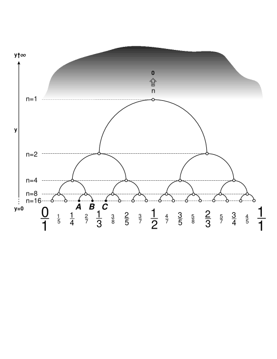
Figure 12: The 3–branching Cayley tree. The barriers are located at the rational points ordered in the Farey sequence. The the replica limit $n\to 0$ is interpreted as the absence of states (vertices of the tree) when $y\to\infty$.

One of the merits of our construction based on the Dedekind $\eta$–function consists in the possibility to change continuously the number of ultrametric barriers and their heights by varying the parameter $y$, and hence to change continuously the number of states $n$ of the RSB matrix. Let us remind that the standard 3–branching Cayley tree being isometrically embedded in the space ${\cal H}=\{z|\,{\rm Im}\,z>0\}$ becomes a ”continuous” structure: one can define the smoothed neighborhood of maxima of the function $f(z)$ in the half–plane $y={\rm Im}\,z>0$—see fig.1. For instance, our construction allows us to increase continuously the number of states $n$ from, say, $n=1$ to $n=2$ changing correspondingly the parameter $y$ in the interval $[y_{n=1},y_{n=2}]$, where $y_{n=1}=\frac{\sqrt{3}}{6}$ and $y_{n=2}=\frac{\sqrt{3}}{14}$.

Our geometric construction based on the isometric embedding of the Cayley tree into the complex plane permits us to consider also the opposite limit—the case when $n$ is formally less than 1. This case means the absence of any states in the RSB matrix ($n=0$). As one sees from figs.1 and 2, the function $f(z)$ has no longer local maxima above the value $y\equiv{\rm Im}\,z>\frac{\sqrt{3}}{2}$. As soon as we have identified the local maxima of the function $f(z)$ with the vertices (states) of the Cayley tree, we conclude that the absence of any states of RSB matrix means the absence of local maxima of the function $f(z)$. Thus, the limit $n\to 0$ we interpret as $y\to\infty$. This claim is based on the behavior of the function $f(z)$ in the upper half–plane. The correspondence of the limits $n\to 0$ and $y\to\infty$ is schematically illustrated in the fig.12. The geometrical interpretation of number of replica states in the region $0<n<1$ makes the physical statement about the ”analytic continuation $n\to 0$” more formal. Actually, let us recall the definition of the hyperbolic distance ${\cal L}$ in ${\cal H}(z|{\rm Im}\,z>0)$ between two points $z_{0}=(x_{0},y_{0})$ and $z=(x,y)$:

$$\cosh{\cal L}=1+\frac{(x-x_{0})^{2}+(y-y_{0})^{2}}{y_{0}\,y}$$ (39)

As we have seen, the hyperbolic distance ${\cal L}$ is the continuous analog of the number of Cayley tree generations, $L$, what permits us to define the number of replica states $n$ as

$$n=e^{{\rm const}\,{\cal L}}$$ (40)

As $y\to 0$, we can replace $\cosh{\cal L}$ with the leading exponential term. This way we arrive at the standard relation $e^{\cal L}=\frac{2y}{y_{0}}$. Hence,

$$\frac{e^{\cal L}}{2}+\frac{e^{-\cal L}}{2}\bigg{\backslash}\;\;=\frac{(x-x_{0})^{2}+y_{0}^{2}}{y_{0}\,y}$$ (41)

neglecting the second term in the left-hand side of (41), we get

$${\cal L}=-\ln y+c_{1}\qquad(y\to 0)$$

where $c_{1}=\ln\frac{2((x-x_{0})^{2}+y_{0}^{2})}{y_{0}}$.

However if $y\to\infty$, eq.(39) gives

$$\frac{e^{\cal L}}{2}\bigg{\backslash}\;+\frac{e^{-\cal L}}{2}=\frac{y}{y_{0}}$$ (42)

where according to the physical condition $n\to 0$ and eq.(40), we have to take another branch of the function ${\rm arccosh}(...)$, corresponding to the negative values of ${\cal L}$. This leads to the following definition of ${\cal L}$:

$${\cal L}=-\ln y+c_{2}\qquad(y\to\infty)$$ (43)

where $c_{2}=\ln\frac{y_{0}}{2}$. As $y\to\infty$, the hyperbolic distance ${\cal L}$, defined according to (43) tends to $-\infty$. Equation (43) is consistent with the definition (40) of number of replicas $n$ in the region $0<n<1$.

It would be very desirable to check how our conjecture works in the models possessing the RSB symmetry of the order parameter. We expect that our construction might be useful for the investigation of aging phenomena considered from the point of view of the diffusion in the whole ultrametric space ${\cal H}(z|{\rm Im}\,z>0)$.

- (1) R.Rammal, G.Toulouse, M.A.Virasoro, Rev. Mod. Phys., 58 (1986), 765
- (2) L.Brekke, P.G.O.Freund, Phys. Rep., 233 (1993) 1
- (3) V.S.Vladimirov, I.V.Volovich, E.I.Zelenov, p-Adic Analysis and Mathematical Physics (WSPC: Singapore, 1994)
- (4) M.Mezard. G.Parisi, M.Virosoro, Spin Glass Theory and Beyond, (WSPC: Singapore, 1987)
- (5) G.Parisi, Phys.Rev.Lett, 43 (1979) 1754; J.Phys.A: Math.Gen., 13 (1980) L115, 1101, 1887
- (6) V.A.Avetisov, A.V.Bikulov, S.V.Kozyrev, J.Phys. A: Math.Gen., 32 (1999) 8785
- (7) G.Parisi, N.Sourlas, Eur.Phys.J., 14 (2000), 535
- (8) V.A.Avetisov, A.V.Bikulov, S.V.Kozyrev, V.A.Osipov, J.Phys. A: Math.Gen., 35 (2002) 177
- (9) V.A.Avetisov, A.K.Bikulov, V.A.Osipov, J.Phys. A: Math.Gen., 36 (2003) 4239
- (10) D.M.Carlucci, C.De Dominicis, Comptes Rendus Ac.Sci.Ser.IIB Mech.Phys. Chem.Astr., 325 (1997) 527
- (11) C.De Dominicis, D.M.Carlucci, T.Temesvari, Journal de Physique I (France) 7 (1997) 105
- (12) A.Terras, Harmonic Analysis on Symmetric Spaces and Applications I, (Springer: New York, 1985)
- (13) K.Chandrassekharan, Elliptic Functions (Springer: Berlin, 1985)
- (14) P.Di Francesco, D.Senechal, P.Mathieu, Conformal Field Theory (Springer: Berlin, 1996)
- (15) A.T.Ogielski, D.L.Stein, Phys.Rev.Lett., 55 (1985), 1634
- (16) C. P. Bachas and B. A. Huberman, J.Phys.A:Math.Gen., 20 (1987) 4995
- (17) W.Magnus, Noneuclidean Tesselations and their Groups (Acad.Press: London, 1974)
- (18) A.F.Beardon, The Geometry of Discrete Groups (Springer: Berlin, 1983)