High Energy Dynamics of the Single Impurity Anderson Model

Abstract

The quantitative control of the dynamic correlations of single impurity Anderson models is essential in several very active fields. We analyze the one-particle Green function with a constant energy resolution by dynamic density-matrix renormalization. In contrast to other approaches, sharp dominant resonances at high energies are found. Their origin and importance are discussed.

Single impurity models are at the very basis of the description of strong correlation phenomena. Landmarks are the Kondo problem kondo64 and the single impurity Anderson model (SIAM) ander61 , for a review see Ref. hewso93, .

The interest in the quantitative analysis of SIAMs has been intensified considerably by the advent of a systematic mapping of strongly correlated lattice models to effective SIAMs supplemented by a self-consistency condition. This is the key point of dynamic mean-field theory (DMFT) jarre92 ; georg92a which is based on an appropriate scaling of the non-local parts of the Hamiltonian metzn89a ; mulle89a , for reviews see Ref. prusc95, ; georg96, . In recent years, the DMFT is applied very successfully in combination with ab-initio density functional calculations anisi97 ; licht98 . In this way, the unbiased knowledge about the bands could be enhanced by the inclusion of interaction effects between the excited quasi-particles. It turned out that the combination of density functional results and DMFT makes the quantitative understanding of spectroscopic data possible held01b .

So far, the methods applied to the SIAM were designed to capture the low-energy physics, in particular the fixed points and the thermodynamics krish80a ; schlo82 . The numerical renormalization group (NRG) was later extended to calculate also dynamic, i.e., spectral information. It provides reliable data on the scale of the Kondo temperatures $T_{\rm K}$ , see Ref. hewso93, ; bulla00a, and references therein. On larger scales, the energy resolution is less well-controlled.

But in various applications the behavior at higher energies is important to achieve quantitative accuracy. For instance, the self-consistency cycle of the DMFT mixes modes at all energies. Hence, excellent quantitative control over the dynamics at high energies is indispensable, even if finally only the behavior at low energies matters.

Another application is the optical control of isolated $S=1/2$ impurities or quantum dots coupled to narrow bands. If the impurities differ so that the energy between the singly occupied ground state and the excited double occupancy differs, they can be switched selectively from the ground state to the double occupancy (and back) by shining light at the resonant frequency onto the sample. The life-time of the double occupancy, i.e., the inverse line width of the resonance, determines how well the resonance condition has to be met, how selective the switching can be, and how stable the excited state is.

In view of the above, we perform a numerical investigation which aims to describe both the low-energy dynamics and the high-energy dynamics quantitatively. To this end, we use an energy resolution which is constant for all energies. Features at low energies are not as delicately resolved as by NRG, but in return features at high energies are much better under control. We apply the dynamic density-matrix renormalization (D-DMRG) hallb95 ; kuhne99a ; hovel00 to compute the one-particle propagator. The DMRG is a real-space approach white92 ; white93 ; pesch98 which works best for open boundary conditions so that it is particularly well-suited to treat impurity problems.

The model investigated at zero temperature is the symmetric Anderson model

$$\mathcal{H}=\sum_{\sigma}\epsilon_{d}n_{d,\sigma}+Un_{d,\downarrow}n_{d,\uparrow}+V\sum_{\sigma}(d_{\sigma}^{\dagger}c_{0,\sigma}^{\phantom{\dagger}}+\text{h.c.})$$

$$+\sum_{n,\sigma}\gamma_{n+1}\left(c_{n,\sigma}^{\dagger}c_{n+1,\sigma}^{\phantom{\dagger}}+\text{h.c.}\right)+\sum_{n,\sigma}\epsilon_{n}c_{n,\sigma}^{\dagger}c_{n,\sigma}^{\phantom{\dagger}}\$$ (1)

with arbitrary density of states (DOS) $\rho_{0}(\omega)$ of the $U=0$ one-particle Green function $G_{0}(\omega)$ of the $d$-electron. The parametrization in (1) is chosen such that the coefficients $(\epsilon_{n},\gamma_{n})$ are the continued fraction coefficients of the hybridization function

$${\Gamma}(\omega)=\frac{V^{2}}{\omega-\epsilon_{0}-{\displaystyle\frac{\gamma_{1}^{2}}{\omega-\epsilon_{1}-{\displaystyle\frac{\gamma_{2}^{2}}{\omega-\cdots}}}}}\ .$$ (2)

This model has particle-hole symmetry iff $\epsilon_{d}=-U/2$ and $\epsilon_{n}=0$ for all $N\geq 0$. The representation as continued fraction viswa94 (see Fig. 1a) is optimum for the DMRG which is designed for chains. We look at a generic situation with finite band width $W=2D$. For simplicity we choose a $\Gamma(\omega)$ with semi-elliptic DOS, i.e., $\gamma_{n}=D/2$. For $V=D/2$, the free DOS $\rho_{0}(\omega)=2\sqrt{D^{2}-\omega^{2}}/(\pi D^{2})$ is also semi-elliptic.

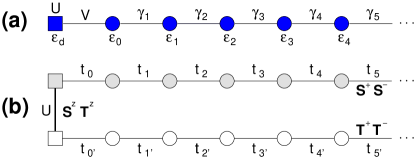
Figure 1: (a) Single impurity model with the bath as half-infinite chain. (b) equivalent spin model: $T$-spins come from $\uparrow$-fermions, $S$-spins from $\downarrow$-fermions.

The problem illustrated in Fig. 1a is mapped by two standard Jordan-Wigner transformations to two $XY$ spin $1/2$ chains, the $S$-chain and the $T$-chain. The $S$-chain results from the $\uparrow$ fermions, the $T$-chain from the $\downarrow$ fermions. They are coupled at site zero where the density-density coupling is mapped to the product of $z$-components. The resulting chain is depicted for the symmetric SIAM in Fig. 1b. The couplings are given by $t_{0}=t_{0^{\prime}}=V$ and $t_{i}=t_{i^{\prime}}=\gamma_{i}$ for $i\geq 1$. The mapping from fermions to spins avoids the fermionic Fock space which would imply numerically difficult long-range effects. The mapping makes the Hilbert space the direct product of the local Hilbert spaces at each site.

The DMRG can easily determine the ground state $|0\rangle$ and its energy $E_{0}$ for a finite chain. So the chain in Fig. 1b is truncated such that there are $L$ spins in the upper and in the lower part of the chain corresponding originally to a truncated bath of $L-1$ fermions plus the impurity. The dynamic quantity we are interested in is the retarded Green function at zero temperature

$$G^{>}(\omega+i\eta)=\langle 0|\mathbf{S}_{0}^{-}(\omega+i\eta-(\mathcal{H}-E_{0}))^{-1}\mathbf{S}_{0}^{+}|0\rangle$$ (3)

where the superscript ^> implies that (3) represents only the part of the usual Green function at non-negative frequencies. In the symmetric case, the complete function is recovered by $G(\omega+i\eta)=G^{>}(\omega+i\eta)-G^{>}(-\omega-i\eta)$. In the asymmetric case, $G^{<}(\omega+i\eta)=\langle 0|\mathbf{S}_{0}^{+}(\omega+i\eta-(\mathcal{H}-E_{0}))^{-1}\mathbf{S}_{0}^{-}|0\rangle$ must be determined separately whereby $G(\omega+i\eta)=G^{>}(\omega+i\eta)-G^{<}(-\omega-i\eta)$ is obtained. We stress that $G(\omega+i\eta)$ is the fermionic propagator even though it is computed in terms of spins after the Jordan-Wigner mapping.

The key idea of the dynamic DMRG is to include the real and the imaginary part of the correction vector $|c\rangle$ in the target states of a standard DMRG algorithm kuhne99a ; hovel00 . The natural choice is $|c\rangle=(\omega+i\eta-(\mathcal{H}-E_{0}))^{-1}\mathbf{S}_{0}^{+}|0\rangle$. The computation of $|c\rangle$ is numerically the most demanding step due to the inversion of an almost singular non-hermitean matrix. We prefer to stabilize this inversion by optimized algorithms freun93a instead of using the variational approach proposed by Jeckelmann jecke02 which requires a minimization in a high-dimensional Hilbert space.

The numerical calculations cannot be performed for $\eta=0$. Even small values of $\eta$ are very time consuming. So we compute first $G(\omega+i\eta)$ at finite $\eta$. The spectral density $\rho^{(\eta)}(\omega)=-\frac{1}{\pi}\Im G(\omega+i\eta)$ can be seen as the actual spectral density $\rho(\omega)$ convoluted by the Lorentzian $\rho_{\text{L}}(\omega)=(\eta/\pi)/(\omega^{2}+\eta^{2})$ of width $\eta$. Hence it is possible to retrieve $\rho(\omega)$ by deconvolution. A standard technique for deconvolution is Fourier transformation, realized best by fast Fourier transforms, division by $\exp(-\eta\tau)$ plus low-pass filtering, and the inverse transform. A flexible alternative with similar properties is the explicit matrix inversion of the convolution procedure gebha03 .

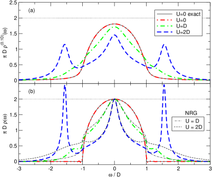
Figure 2: (a) Spectral densities for $V=D/2$ broadened by $\eta=0.1D$. Chain length $L=80$ fermionic sites; 128 DMRG states kept. (b) Spectral densities from (a) deconvoluted in the time domain. NRG data ($\Lambda=1.8$, 1500 states) depicted by thin dashed lines. The exact curves represent the analytic $L=\infty$ results.

In Fig. 2a, generic broadened spectral densities are plotted as they are computed by D-DMRG. Obviously, the value $\rho^{(\eta)}(0)$ is not independent of $U$. Increasing the chain length $L$ does not lead to any significant change in the data (not shown). Fig. 2b displays the deconvoluted data. The deconvolution works very well except for some slight overshooting in regions where the spectral density changes rather abruptly. In particular, the value $\rho(0)$ is pinned to $D/(2\pi V^{2})$ independent of $U$ as required by Friedel’s sum rule and the density of states rule lutti60b ; lutti61 ; ander91 ; hewso93 . We take this fact as convincing evidence for the reliability of the numerical algorithm.

The central peak at $\omega=0$ is the Abrikosov-Suhl resonance (ASR). For larger $U$ (smaller $V$) its width decreases rapidly so that the ASR is very difficult to resolve nishi03 unless more elaborate deconvolution schemes are devised raas04a . So a quantitative analysis of the ASR is postponed to future work.

For comparison, the thin dashed lines in Fig. 2b depict standard NRG data bulla98 ; bulla00a . For small frequencies NRG is well-controlled. Indeed, for $|\omega|\lessapprox D/3$, NRG and D-DMRG data agree excellently lending further support to the D-DMRG approach. Outside the band, the NRG spectra appear to be too wide due to the chosen constant broadening on a logarithmic mesh. This broadening does not account for the absence of states outside the bare band. The NRG does not possess intrinsic information about the peak widths. The position of the high energy peak in the raw NRG data, however, coincides with the D-DMRG result.

An increase in $U$ leads to the formation of Hubbard satellites below and above the free band (Fig. 2). They are situated at energies $\omega_{\rm up/low}=\pm(U/2+\delta_{\rm shift}),\delta_{\rm shift}>0$ and become more pronounced on increasing $U$ in two ways. They capture more weight and they become sharper. For $T_{\text{K}}\to 0$ the weight reaches 1/2, see Ref. ander91, . The sharpening has not been discussed quantitatively before although the extended non-crossing approximation prusc89 provides sharp satellites if they lie outside the bare bands, see e.g. Fig. 1 in Ref. ander91, . Recently, indications have occured gebha03 that other standard algorithms overestimate the width of the Hubbard satellites. The exaggerated width of the NRG data at high energies results from the Gaussian broadening of the order of the energy range sakai89 .

To investigate the line shapes of the satellites we plot them for various values of $U$ and $V$ in Fig. 3. The ASR at $\omega=0$ is not displayed since it is too much smeared out at $\eta=0.1D$ for larger values of the interaction. The shifts $\delta_{\rm shift}$ increase on increasing $V$; they decrease on growing interaction $U$. The widths behave qualitatively similar. A complete deconvolution suffers unfortunately from severe overshooting due to the sharpness of the resonance. To make the analysis nonetheless quantitative we fit the broadened data by Lorentzians plus an offset (Fig. 3). These fits work very well for large values of $U$ and not too large values of $V$.

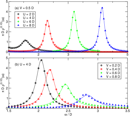
Figure 3: D-DMRG data of the upper Hubbard satellite at $\eta=0.1D$. Thin lines are fits with Lorentzians and an offset $\propto\eta_{\rm eff}/(\eta_{\rm eff}^{2}+(\omega-\omega_{\rm up})^{2})+C$. The fits were done for the intervals shown. (a) dependence on $U$ at constant $V$ ($L=80$); (b) dependence on $V$ at constant $U$ ($L=40$).

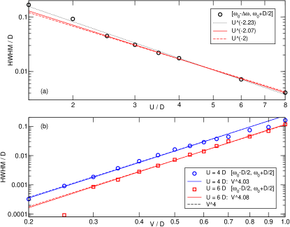
Figure 4: Widths (symbols) of the Hubbard satellites as found from the fits in Fig. 3. The fit intervals are given in the legend. The lines show various power law fits. (a) dependence on $U$ at $V=D/2$; (b) dependence on $V$.

To deduce the true width of the Hubbard satellite we assume that it is well described by a Lorentzian. The width $\eta_{\rm eff}$ of the convolution of two Lorentzians of widths $\eta_{1}$ and $\eta_{2}$ is $\eta_{\rm eff}=\eta_{1}+\eta_{2}$. From the effective widths $\eta_{\rm eff}$ we deduce the true half-widths at half-maximum (HWHM) of the Hubbard satellite by subtracting the artificial broadening $\eta$, i.e., HWHM $=\eta_{\rm eff}-\eta$. In Fig. 4, the widths are depicted as function of $U$ and of $V$. The results show that the HWHM are proportional to $V^{4}/U^{2}$. The deviations for smaller widths must be attributed to the numerical constraints, e.g., finite $\eta$ and finite chain length $L$. The deviations for larger widths, mainly for larger values of $V$ and smaller values of $U$ result from the vicinity of the bare bands.

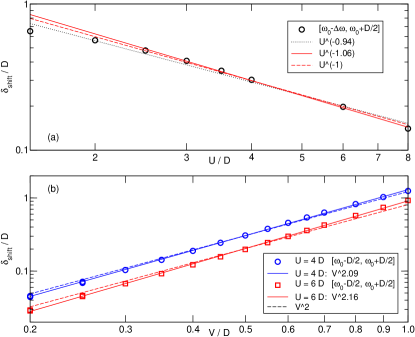
Figure 5: Position shifts of the Hubbard satellites analyzed like the widths in Fig. 4; (a) $V=D/2$; (b) see legend.

Fig. 5 displays the analogous analysis for the shifts $\delta_{\rm shift}$ of the satellite positions. Again, strong evidence for power law behavior is found, namely $\delta_{\rm shift}\propto V^{2}/U$.

How can the above findings be understood? Let us start by the positions. The energy levels of isolated impurities, i.e., $V=0$ are at $\pm U/2$ schri66 . Switching on $V$ mixes the impurity levels with the bath states which lie in the interval $[-D,D]$. If $U$ is large compared to $D$ second order perturbation in $V$ implies that the impurity levels are repelled from the bath states. The shift should be of the order of $J=8V^{2}/U$, see Eq. (11) in Ref. schri66, , which agrees nicely with the power laws in Fig. 5.

The widths of the satellites have been discussed quantitatively when they lie within the bare band logan98 . If the satellites lie outside, perturbation theory in $U$, to second order or the random phase approximation, implies that a finite width is to be expected at least for $U<6D$. But the reasoning in powers of $U$ is not helpful for $U>6D$ and it does not explain the power laws found. So we return to perturbing in powers of $V$. The impurity levels mix with particle-hole excitations in the bands, see Eq. (10a) in Ref. schri66, . In the symmetric case the doubly occupied electron and hole state are degenerate so that mixing with particle-particle (or hole-hole) states matters also, see Eq. (12) in Ref. schri66, . The mixing is of order $J=8V^{2}/U$. So Fermi’s golden rule implies a life time of $J^{2}N_{0}$ where $N_{0}$ measures the density of states with which the impurity level mixes; $N_{0}$ is of the order of $D^{-1}$. Indeed, HWHM $\propto J^{2}$ explains conclusively the data of Fig. 4.

So far, the width of the Hubbard satellites for $U>2D$ was extracted under the assumption that the satellites are Lorentzians. Further investigations of the line shape are urgently called for. Numerically, improvements of the resolution are necessary to determine the line shape of the satellites explicitly. Analytically, the quantitative argument for the widths must be supplemented by an explicit calculation of the line shapes for $V^{2}/U\to 0$.

In summary, we have investigated the dynamic propagator of the SIAM by D-DMRG. This powerful large-scale algorithm provides information with a constant energy resolution. Up to moderate interactions $U\approx 2D$, deconvolution yields the explicit spectral densities. For larger interactions, the width of sharp resonances can be extracted by fitting Lorentzians. In particular, we analyzed the positions and widths of the Hubbard satellites. The shifts are of order $V^{2}/U$ due to level repulsion; the line widths are of order $V^{4}/U^{2}$.

Especially the sharpness of Hubbard peaks is missed by other zero temperature algorithms for the SIAM. Hence the D-DMRG is a very valuable complementary tool. Position and width of the Hubbard satellites are important for several widely used applications, e.g., in the self-consistency cycle of the DMFT.

Acknowledgements  We thank R. Bulla, L. Craco, M. Grüninger, T. Hövelborn, D. Logan, H. Monien, and E. Müller-Hartmann for helpful discussions and the DFG for financial support (Uh 90/3-1 and SFB 608).

References

- (1) J. Kondo, Prog. Theor. Phys. 32, 37 (1964).
- (2) P. W. Anderson, Phys. Rev. 124, 41 (1961).
- (3) A. C. Hewson, The Kondo Problem to Heavy Fermions (Cambridge University Press, Cambridge, 1993).
- (4) M. Jarrell, Phys. Rev. Lett. 69, 168 (1992).
- (5) A. Georges and G. Kotliar, Phys. Rev. B 45, 6479 (1992).
- (6) W. Metzner and D. Vollhardt, Phys. Rev. Lett. 62, 324 (1989).
- (7) E. Müller-Hartmann, Z. Phys. B 74, 507 (1989).
- (8) T. Pruschke, M. Jarrell, and J. K. Freericks, Adv. Phys. 44, 187 (1995).
- (9) A. Georges, G. Kotliar, W. Krauth, and M. J. Rozenberg, Rev. Mod. Phys. 68, 13 (1996).
- (10) V. I. Anisimov et al., J. Phys.: Condens. Matter 9, 7359 (1997).
- (11) A. I. Lichtenstein and M. I. Katsnelson, Phys. Rev. B 57, 6884 (1998).
- (12) K. Held et al., Int. J. Mod. Phys. B 15, 2611 (2001).
- (13) H. R. Krishna-murthy, J. W. Wilkins, and K. G. Wilson, Phys. Rev. B 21, 1003 and 1044 (1980).
- (14) P. Schlottmann, Z. Phys. B 49, 109 (1982).
- (15) R. Bulla, in Advances in Solid State Physics, edited by B. Kramer (Vieweg Verlag, Braunschweig, 2000) 40, 129.
- (16) K. A. Hallberg, Phys. Rev. B 52, 9827 (1995).
- (17) T. D. Kühner and S. R. White, Phys. Rev. B 60, 335 (1999).
- (18) T. Hövelborn, diploma thesis, Bonn/Köln, 2000; available at www.thp.uni-koeln.de/gu.
- (19) S. R. White, Phys. Rev. Lett. 69, 2863 (1992).
- (20) S. R. White, Phys. Rev. B 48, 10345 (1993).
- (21) I. Peschel, X. Wang, M. Kaulke, and K. Hallberg, Density-Matrix Renormalization, Vol. 528 of Lecture Notes in Physics (Springer, Berlin, 1999).
- (22) V. S. Viswanath and G. Müller, The Recursion Method; Application to Many-Body Dynamics, Vol. m23 of Lecture Notes in Physics (Springer-Verlag, Berlin, 1994).
- (23) R. W. Freund, SIAM J. Sci. Comput. 14, 470 (1993).
- (24) E. Jeckelmann, Phys. Rev. B 66, 045114 (2002).
- (25) F. Gebhard et al., Eur. Phys. J. B in press, cond-mat/0306438.
- (26) J. M. Luttinger, Phys. Rev. 119, 1153 (1960).
- (27) J. M. Luttinger, Phys. Rev. 121, 942 (1961).
- (28) F. B. Anders, N. Grewe, and A. Lorek, Z. Phys. B 83, 75 (1991).
- (29) S. Nishimoto and E. Jeckelmann, J. Phys.: Cond. Matter in press, cond-mat/0311291.
- (30) C. Raas and G.S. Uhrig, in preparation
- (31) R. Bulla, A. C. Hewson, and T. Pruschke, J. Phys.: Condens. Matter 10, 8365 (1998).
- (32) T. Pruschke and N. Grewe, Z. Phys. B 74, 439 (1989).
- (33) O. Sakai, Y. Shimizu, and T. Kasuya, J. Phys. Soc. Jpn. 58, 3666 (89).
- (34) J. R. Schrieffer and P. A. Wolff, Phys. Rev. 149, 491 (1966).
- (35) D. E. Logan, M. P. Eastwood, and M. A. Tusch, J. Phys.: Condens. Matter 10, 2673 (1998).