Simulation of Cu-Mg metallic glass: Thermodynamics and Structure

Abstract

We have obtained effective medium theory (EMT) interatomic potential parameters suitable for studying Cu-Mg metallic glasses. We present thermodynamic and structural results from simulations of such glasses over a range of compositions. We have produced low-temperature configurations by cooling from the melt at as slow a rate as practical, using constant temperature and pressure molecular dynamics. During the cooling process we have carried out thermodynamic analyses based on the temperature dependence of the enthalpy and its derivative, the specific heat, from which the glass transition temperature may be determined. We have also carried out structural analyses using the radial distribution function (RDF) and common neighbor analysis (CNA). Our analysis suggests that the splitting of the second peak, commonly associated with metallic glasses, in fact has little to do with the glass transition itself, but is simply a consequence of the narrowing of peaks associated with structural features present in the liquid state. In fact the splitting temperature for the Cu-Cu RDF is well above $T_{g}$. The CNA also highlights a strong similarity between the structure of the intermetallic alloys and the amorphous alloys of similar composition. We have also investigated the diffusivity in the supercooled regime. Its temperature dependence indicates fragile-liquid behavior, typical of binary metallic glasses. On the other hand, the relatively low specific heat jump of around $1.5k_{B}/\mathrm{at.}$ indicates apparent strong-liquid behavior, but this can be explained by the width of the transition due to the high cooling rates.

I Introduction

Metallic glasses Greer (1995); Johnson (1999) have generated considerable scientific interest since they were discovered 40 years ago, due to their unusual magnetic and mechanical properties, as well as wear and corrosion resistance, and their glass-forming ability per se. This interest has substantially increased since the discovery of the so-called bulk metallic glasses (BMGs) or bulk amorphous alloys, by Inoue Inoue et al. (1991) and Johnson.Peker and Johnson (1993) The ability to create samples with thicknesses in the mm or cm range, rather than $\mu$m thick ribbons, greatly increases the applicability of the materials, as well as the range of measurements that can be performed on them. This is particularly true in the case of mechanical testing, and recently measurements of properties such as fracture toughness, fracture morphology and crack-tip plasticity have been made.Fedorov and Ushakov (2001); Flores and Dauskardt (2001); Schneibel et al. (2001); Gilbert et al. (1997)

The mechanisms of plastic deformation are of particular interest in metallic glasses in view of the fact that there are no obvious topological defects which might play a role analogous to crystal-dislocations, allowing slip to take place in small increments. Thus metallic glasses tend to have very high flow stresses.Greer (1995) A complete understanding of plastic deformation must include the following two parts: (i) detailed knowledge of the elementary events that constitute plastic flow and (ii) a practical continuum theory which uses this knowledge to make predictions of macroscopic behavior (a recent such theory is the so-called Shear Transformation Zone (STZ) theoryFalk and Langer (1998); Langer and Pechenik (2003)). The motivation for the present work is a desire to tackle item (i) using the tools of modern materials simulations, specifically: realistic potentials, system sizes as large as feasible and necessary, and sophisticated analysis and visualization techniques. The first step, addressed in this paper, is to create appropriate interatomic potentials, generate glassy configurations, and study the thermodynamics and structure of the system, in order to understand it as a glass-forming one. Simulations of mechanical properties will be presented in future publications. The phrase “realistic potentials” refers to contemporary potentials commonly used for metals, including effective medium or embedded atom-type potentials, or pseudopotential-based pair potentials, as opposed to Lennard-Jones potentials, which are commonly used (with two components) to model metallic glasses. Kob and Andersen (1995a, b); Sastry et al. (1998); Utz et al. (2000); Lacks (2001); Varnik et al. (2003) Such potentials are especially useful because they allow quantitative comparison with experiments of properties such as glass transition temperature, and, later, mechanical properties.

In this paper we present molecular dynamics simulations of the binary alloy Cu_xMg_1-x. Mg-based BMGs such as Mg₆₀Cu₃₀Y₁₀Inoue et al. (1991); Busch et al. (1998); Wert et al. (2001); Wolff et al. (2003) are of interest because their weight is low, being dominated by Mg, but their strength can be comparable to high-strength steel. We have chosen to study the binary alloy because (i) it is simpler to optimize a potential for two species than for three and (ii) it is easier to study dependence on a single composition-parameter than on two. Our intent to use realistic potentials necessitates an attempt to create as realistic a glass as possible with those potentials. It is thus important to characterize the system as a glass-forming and alloying one as completely as possible.

The Cu-Mg equilibrium phase diagram is shown in Fig. 1. Experimentally it forms a glass over a range of compositions from 9–42 at. % (complete glass formation over 12–22 %, which includes the eutectic composition 14.5 %).Sommer et al. (1980) It is not a BMG, since it can only be formed by melt-spinning at high cooling rates. The cooling rates in the simulations are necessarily even higher and allow glassy configurations to be created over almost the entire range of compositions. It is worth studying the experimentally inaccessible states as part of the process of detecting trends in material properties as a function of composition; it is the crystal-nucleation timescale, lying between the simulation and experimental timescales, which makes the difference between crystalline and amorphous phases—if just a few orders of magnitude gain in cooling rate could be experimentally realized, there is reason to believe these states would be as stable as the actual glassy configurations currently realizable by experiment.

Because the crystallization rates are high, there are limited experimental measurements of the thermodynamic properties of Mg-Cu glasses, and thus it is of interest to study these in the simulations before moving on to mechanical properties. In the process we find some interesting results regarding structural changes in the super cooled regime (steady growth of icosahedral order and evidence of restructuring thermodynamics). Additionally we make some observations on the question of the fragility of this system. The next section will discuss some aspects of the theory of glass formation in alloys, as applied to the Cu-Mg system. Section III will discuss simulation methods, including the fitting of the interatomic potential. Sections IV and V discuss characterization of the glass transition and of structural properties respectively. The last section is the discussion.

II Glass formation in the Mg-Cu system

One approach to the theory of metallic glass formation is based on pseudopotential-derived interatomic pair potentials,Hafner (1980, 1987) and emphasizes the coincidence of bond lengths with potential minima. We will not be using such potentials; in fact many aspects of glass formation are purely geometrical (packing of spheres) and phase-energeticHafner (1980) (comparison with competing crystalline phases). Frank and Kasper Frank and Kasper (1958, 1959) pointed out that many complex intermetallic structures can be understood in terms of tetrahedral close-packing of spheres. Examples of so-called Frank-Kasper (FK) phases include the Laves phases (C14, C15, C36) and $\mu$, $\chi$ and $\sigma$ phases. The high packing fraction and coordination numbers suggest directional bonding does not play a role. The closest packing of spheres of equal size is achieved with a tetrahedron (79%), but tetrahedra cannot fill space—the best one can do is make an icosahedron out of twenty slightly distorted tetrahedra, but this cannot be repeated periodically, so in crystals one has the fcc (e.g. Cu, $a=3.61$Å) and hcp (e.g. Mg, $a=3.21$Å, $c=5.21$Å) structures, with 74% packing.

In the Cu-Mg system there is indeed a Laves phase, Cu₂Mg. This is not surprising given that the ideal Laves packing is achieved with a radius ratio of 1.225 (Ref. Hafner, 1987, p.59), which is close to that of Mg and Cu (1.256 using the Goldschmidt radii, based on nearest neighbor distances of the pure metals). This phase is quite stable simply because having a majority of smaller atoms allows a greater packing fraction. On the other hand Mg₂Cu, with the larger atoms in the majority, is not as stable an alloy.Hafner (1980) Mg-Cu is in a class of metallic glass formers which include simple metal-transition metal binary alloys and are characterized by a Laves phase when the small atom (Cu) is in the majority, and a glass when the larger atom is. In Cu₂Mg the Cu atoms have CN12 icosahedral coordination and the Mg atoms are 16-coordinated, surrounded by so-called Frank-Kasper 16-hedra (more specifically, Friauf polyhedra).

Glass formation in a binary alloy appears to be favored by the same criteria that favor the formation of FK phases: large, negative heats of formation, non-directionality of bonding, and a tendency to maximize packing fraction. In general one finds that for compositions between intermetallics (for example near eutectics), where the equilibrium phase diagram shows a two-phase mixture, the amorphous phase is more stable than any single crystalline phase. In the region of the phase diagram where FK phases appear, glass formation typically loses out in the competition experimentally, presumably because the nucleation of the Laves phase is rather easy. In the Cu-Mg system, the region of experimental glass formation is on the Mg-rich side, where the competing crystalline phase, Mg₂Cu, is quite complex (48 atoms in the unit cell).

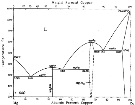
Figure 1: Equilibrium phase diagram for Mg-Cu (from Ref. Massalski, 1990)

III Simulation methods

III.1 Potentials

The interatomic potential we use is the effective medium theory (EMT),Jacobsen et al. (1987, 1996) fit to data obtained from density functional theory (DFT) calculations and experiment. This has previously been applied to fcc metals, in particular late transition and noble metals and has been of great use in studying mechanical properties of crystalline metals.Schiøtz et al. (1999); Schiøtz and Jacobsen (2003) As Mg crystallizes in hcp with an almost ideal $c/a$-ratio of $1.624$ (ideal is $\sqrt{8/3}=1.633$), indicating little directional bonding, we might expect it to be reasonably well described by an appropriately optimized EMT potential.

EMT uses seven parameters for each element. A set of parameters for Cu exists but these have been optimized for simulations of pure, crystalline Cu (where for example particular attention was paid to the stacking fault energy, which is of no concern in amorphous materials). For the amorphous alloys, it is important that the formation energies are reasonable, in particular that they are negative (otherwise the system will simply separate into regions of pure Cu and regions of pure Mg).

Thus we have (re-)fit the parameters of both elements, taking into account basic properties such as lattice constants, cohesive energies and elastic constants of the pure elements, as well as the formation energies of the two intermetallic compounds, Mg₂Cu and Cu₂Mg. Due to the near-ideal hcp packing of Mg, its structure differs from fcc only at the second neighbor level. For simplicity, and because the EMT potential is formulated in terms of fcc packing, we used calculated properties of fcc Mg in the fitting, except that the cohesive energy was corrected using the experimental hcp value and the calculated fcc-hcp difference ($23meV$/atom), calculated differences in cohesive energy being expected to be more accurate than calculated cohesive energies themselves.

parameter	Cu	Mg
$s_{0}$	2.67	1.766399
$E_{0}$	-3.51	-1.487
$\lambda$	3.693666	3.292725
$\kappa$	4.943848	4.435425
$V_{0}$	1.993953	2.229870
$n_{0}$	0.063738	0.035544
$\eta_{2}$	3.039871	2.541137

Table 1: EMT parameters for Cu and Mg, in units derived from $eV$ and Å.

property	optimized value	target value
Cu-$E_{\textrm{coh}}$	3.521	3.510
Cu-$a$	3.588	3.610
Cu-$B$	0.891	0.886
Cu-$C_{44}$	0.512	0.511
Cu-$C_{11}$	1.095	1.100
Mg-$E_{\textrm{coh}}$	1.487	1.487
Mg-$a$	4.502	4.520
Mg-$B$	0.242	0.225
Mg-$C_{44}$	0.117	0.115
Mg-$C_{11}$	0.293	0.326
Mg2Cu-$\Delta H$	-0.115	-0.132
Mg2Cu-$a$	5.250	5.320
Cu2Mg-$\Delta H$	-0.159	-0.157
Cu2Mg-$a$	6.943	7.158

Table 2: Properties used in the fitting: the values specified (from DFT/experiment) and the values according to the optimized potential. $B=$ bulk modulus, $a=$ lattice constant.

The optimized EMT coefficients are shown in table 1 and the target and fitted values of the fitting properties are shown in table 2. Note that for the orthorhombic Mg₂Cu, the experimental $b/a$ and $c/a$ were used, as well as the experimental values of the internal coordinates. The alloy formation energies are well-represented. Unlike pair potentials based upon pseudopotentials, the present form of the EMT potentialJacobsen et al. (1996) does not incorporate the Friedel oscillations, and the idea that stability of intermetallic compounds is determined by the matching of minima of pair potentials to interatomic distancesHafner (1980) does not play a role; the fact that EMT parameters can be chosen to give the correct formation energies of the intermetallic compounds appears to be most important.

III.2 Molecular dynamics

We simulated the cooling of systems of 2048 atoms from the liquid state (above the melting point) down to zero temperature. The compositions ranged from pure Mg to pure Cu, and are labeled by the percentage of Cu. For most simulations we used 21 compositions, increasing in steps of 5% from 0 (pure Mg). The initial state was an fcc lattice with the sites occupied at random by Cu or Mg atoms in accordance with the overall composition. There was no initial heating phase; the first stage in the cooling run set the temperature to a value well above the melting point (values ranged from 1392 K for Mg ($T_{m}=923K$) to 1857 K for Cu ($T_{m}=1358K$)), making the crystal melt immediately. Two rates of cooling were used; differing in the amount of simulation time at each temperature. Cooling took place in steps of $35K$; the procedure at each temperature stage was as follows: (i) a small number of steps, corresponding to $0.6ps$ (the MD time-step was $2fs$), of constant-volume Langevin thermalization was carried out in order to approximately thermalize the system to the new temperature; (ii) the dynamics was switched to constant-pressure (NPT) dynamics and the system was simulated for an initial equilibration time of $6ps/12ps$; (iii) the system was simulated for a longer time $40ps/120ps$ during which thermal averages of various quantities of interest were taken. This time also contributed to the equilibration of the system. The overall cooling rates were thus close to $0.72K/ps$ ($7.2\times 10^{11}K/s$) and $0.25K/ps$ ($2.5\times 10^{11}K/s$). The NPT dynamics used was a combination of Nose-Hoover and Parrinello-Rahman dynamics, proposed by Melchionna.Melchionna et al. (1993); Melchionna (2000); Holian et al. (1990); Di Tolla and Ronchetti (1993) We turned off shearing, allowing only volume fluctuations, because the liquid state cannot support a shear stress and fluctuations in the periodic box sometimes lead to extreme angles between box vectors and thus problems with the neighbor-locating algorithm. The pressure was zero or a small positive value (this was necessary in some cases when the initial temperature was above the boiling point of pure Mg). For each cooling rate the simulations were run twice with different random number seeds (affecting the distribution of species in the initial lattice and the Langevin dynamics used when the temperature is changed; the NPT dynamics does not use random numbers).

During the averaging period, the pressure, volume, kinetic and potential energies were recorded and averaged. For the purposes of structural analyses so too was the radial distribution function (RDF), both total and separated into contributions from Mg-Mg, Cu-Cu and Mg-Cu. At the end of the averaging time the current configuration was saved, as well as a configuration obtained from it by direct minimization (quenching) using the MDmin minimization algorithm. At a later time the saved configurations from selected temperatures were used for further simulation at that temperature to gather further dynamical and structural information such as diffusion constants and thermally averaged common neighbor analysis (CNA).

Figure 2: Cooling rate dependence of $T_{g}$ for 15% Cu system. Solid symbols, $T_{g}$ from the maximum rate of change of $C_{P}$; open symbols, $T_{g}$ by intercept method. Arrows indicate the cooling rates used for the main simulations. Inset: enthalpy of system at end of cooling run ($T=0$).

Our cooling rates are as slow as in other recent simulations of amorphous metals,Hui et al. (2002); Qi et al. (1999); Posada-Amarillas and Garzon (1996); Lewis (1989) but they are of course larger than experimental rates by several orders of magnitude. In order to check that our results are not significantly affected by this difference, we have cooled one composition, 15% Cu at several faster rates and one slower one. Fig. 2 shows $T_{g}$ and the enthalpy at $T=0$ for these runs. The methods of calculating $T_{g}$ are explained in the next section; only one (intercept) could be used for the very fast runs. It is pretty clear that for the cooling rates used in the main simulation, the dependence of $T_{g}$ on cooling rate has become smaller than the uncertainty in determining $T_{g}$. The enthalpy shows a definite slope still at the lowest cooling rate, amounting to about $1meV$ per order of magnitude cooling rate, which is rather small; also one would expect the curve to flatten out more at even smaller rates. The one significant difference we notice is that crystallization at the Cu-rich end happens at lower Cu-concentrations for slower cooling: the 90% Cu system crystallizes in one run at $0.25K/ps$ but not at all at $0.72K/ps$.

IV Glass transition

Figure 3: Specific heat versus temperature for 15% Cu system, cooling rate $0.72K/ps$. Dashed lines, values from two separate cooling runs, displaced $\pm 0.2$ for clarity. Solid line, average of these two. Solid vertical line, $T_{g}$ from maximum slope of specific heat; solid dashed line, $T_{g}$ from intercept method. Inset: enthalpy (average of the two runs) versus temperature. Dotted lines show the extrapolated straight-line fits from the intercept method.

We see glass transitions in almost all compositions, the exceptions being the pure elements and 95% Cu, which crystallize in fcc/hcp structures (also 90% Cu in one out of two runs at $0.25K/ps$). The first evidence that a glass transition takes place upon cooling appears in the enthalpy versus temperature curve, which shows a change in slope (inset in Fig 3). This suggests a way to determine $T_{g}$ by breaking the curve into two pieces, fitting a straight line to each, and intersecting the two lines obtained. We call this the “intercept-method”. It turns out that this tends to underestimate $T_{g}$ as can be seen by looking at the derivative of the enthalpy, the specific heat (Fig 3), obtained from centered differences. The $T_{g}$ ends up at the leftmost part of the steep part of the curve, whereas one would expect any reasonable definition of $T_{g}$ to be roughly in the center of the transition region (defined as the steep part). Thus we compute $T_{g}$ as the temperature at which the specific heat is changing fastest by taking derivatives again and simply choosing the maximum. This method necessarily yields a $T_{g}$ equal to one of the simulation temperatures, but since the transition region is a few times wider ($150-200K$) than the temperature step in the simulation, one cannot expect to do better (experimentally one sees widths of some tens of $K$, see for example Ref. Busch et al., 1995). In cases where we have two different enthalpy curves for the same system cooled identically but from different starting configurations we average the two enthalpy curves before applying the method, as this gives a smoother $c_{P}$ curve.

The $T_{g}$ we get for 15% Cu is $350K$ which is remarkably similar to the experimental value of $380K$ reported by Sommer et al.Sommer et al. (1980) In runs where crystallization took place, a large spike in the specific heat appeared, corresponding to a step or latent heat in the enthalpy curve. Before looking at the composition dependence of $T_{g}$, we notice that the temperature dependence of $c_{P}$ is quite similar in form to experimental specific heat curves of Zr_41.2Ti_13.8Cu_12.5Ni_10.0Be_22.5 reported by Busch et al. Busch et al. (1995) and of fluorozirconate and tellurite glasses reported by Lin and Navrotsky;Lin and Navrotsky (1997, 1998) there is an increase in specific heat in the supercooled liquid region compared to the high-temperature liquid region. For the tellurites, Lin and Navrotsky identified the source of this as specific structural rearrangements that take place in the liquid prior to the glass transition. We will see in the next section what evidence there is for structural rearrangements in the Cu-Mg supercooled liquid.

Figure 4: $T_{g}$ and $T_{\textrm{split}}$ (upper panel) and $\Delta c_{P}$ (lower panel). Squares: $T_{g}$, $\Delta c_{P}$ at $0.72K/ps$; diamonds at $0.25K/ps$. Triangles: $T_{\textrm{split}}$(Cu) at $0.72K/ps$.

Fig. 4 shows $T_{g}$ and $\Delta c_{P}$, the heat capacity jump (obtained by roughly determining the transition region as the peak in the derivative of $C_{P}$ and taking the difference of $C_{P}$ on either side of the peak) for different compositions and cooling rates. $T_{g}$ rises roughly linearly with increasing fraction of Cu, which presumably reflects a general increase in energy scale as we go from the weakly cohesive (low melting point) Mg to the more strongly cohesive Cu. The fluctuations towards the Cu-rich end are due to the mid-point method’s difficulty handling the somewhat less clean $c_{P}$-data there. The fluctuations in $\Delta c_{P}$ are also due to the imperfect $c_{P}$-data. Nevertheless, it seems clear that $\Delta c_{P}$ has the value of roughly $1.5k_{B}$ per atom, independent of concentration. This is a relatively small amount, which is typical of so-called “strong” glass-formers, which include most BMGs.Busch (2000) In particular the Mg₆₅Cu₂₅Y₁₀ shows a jump of the same order (actually $2k_{B}/\textrm{at.}$).Busch et al. (1998) However, we should be careful about inferring strong-liquid behavior from this measurement; binary alloys typically are not strong glass-formers, Johnson (1999) and below we shall see evidence of fragile-liquid behavior in the diffusivity. The apparent small jump of $C_{P}$ may be a consequence of the width of the transition.

Figure 5: Diamonds: formation enthalpy per atom in final zero-temperature glassy state. Dotted line: formation enthalpy per atom of corresponding (in general two-phase) crystal.

As a partial means of determining how good, meaning how stable or well-annealed, the final configurations are, we consider their enthalpies. We have seen already how the final enthalpy depends on cooling rate (Fig. 2); we now compare to the equilibrium phases, for different compositions. Fig. 5 shows the formation enthalpies as a function of composition. The formation enthalpy is the enthalpy minus the appropriate linear combination of the pure elements’ enthalpies. The appropriate quantity to compare to, also shown in Fig. 5, is the formation enthalpy of the corresponding crystalline phase, which in general is a two-phase mixture (so, e.g., between 33% Cu and 66% Cu it is an appropriate weighting of the formation enthalpies of Cu₂Mg and Mg₂Cu). We notice that the glass formation enthalpy follows quite closely the crystalline one, being 1–4 $kJ/mol$ higher (the exceptions being at 0, 95% and 100% Cu where the system did in fact crystallize). This is quite small and typical of easy glass formers.Johnson (1986, 1999); Greer (1995) For the 15%Cu composition the value $4.2kJ/mol$ was reported by Sommer et al. for the transformation enthalpy from the crystalline to the amorphous state, which is slightly higher than our value of $3.53kJ/mol$—that is, our glass at this composition appears to be a little too stable compared with experiment. This kind of discrepancy can only be due to limitations of the interatomic potential, and not to the high cooling rate. This gives us further confidence that we have created glassy structures which are more or less as stable as they can be.

Figure 6: Diffusion constants in 15% Cu. Squares: Mg; diamonds: Cu. Dotted line: VF fit to high temperature Mg data. Dashed line: Arrhenius fit to low temperature Mg data.

Figure 7: Upper panel: fragility parameter $D^{*}$ of Vogel-Fulcher fits to Cu diffusion constants at selected compositions. Lower panel: location of apparent divergence $T_{0}$ from the same fits.

For selected compositions and selected temperatures, configurations from the cooling runs were used as initial configurations for further simulations in which diffusion constants for the two atomic species were measured. An Arhennius plot for the 15% Cu composition is shown in Fig 6. There is a clear indication of a transition near $1000/T\sim 3K^{-1}$, corresponding to $T\sim 330K$, which is consistent with the $T_{g}=350K$ obtained from the specific heat. For each composition for which diffusion constants were measured, we have fitted the high temperature part of the data to the Vogel-Fulcher (VF) law

$$D=D_{0}\exp(\frac{D^{*}T_{0}}{T-T_{0}})$$ (1)

where $T_{0}$ is the location of the apparent singularity and $D^{*}$ is the so-called fragility parameter. In Fig 7 we show $D^{*}$ and $T_{0}$ obtained from fits of the Cu diffusion constants to the VF law (the Mg values are very similar, the differences being very small compared to the differences from composition to composition). There is a reasonably clear trend towards decreasing $D^{*}$ and increasing $T_{0}$ as the fraction of Cu increases. High values $D^{*}$ are associated with strong glass-formers, the archetypal case of SiO₂ having $D^{*}=100$. Bulk metallic glasses are considered strongBusch (2000) with $D^{*}\sim 20$. So-called fragile glasses have $D^{*}$ around 2. From our diffusion data we get low fragility parameters, in the range 2–4, indicating that the Mg-Cu glasses are somewhat fragile. This is consistent with the experimental fact that this is not in fact a bulk metallic glass. The $T_{0}$ values increase as the fragility decreases, so that the apparent singularity approaches the actual glass transition temperature. These trends, reflecting greater fragility (decreasing $D^{*}$) with increasing Cu composition, are also consistent with the fact that experimentally, amorphous Mg-Cu can only be made at all for Mg-rich compositions, since strong liquids tend to be robust against crystallization (in a strong glass former the melt viscosity is high, making the kinetics slow). Thus, our diffusion results put the binary alloy Mg-Cu at the fragile end. This seems to contradict the suggestion of strong-liquid behavior from the specific heat data. The small $\Delta C_{P}$, may have a simple explanation, however, namely that it has been reduced due to the broadening of the transition in the simulations compared to what one would expect experimentally. This broadening implies that a certain amount of restructuring, that at slower cooling rates would take place above $T_{g}$, in the simulation takes place during and below $T_{g}$. The net enthalpy change (the area under the $C_{P}$ curve) is more or less the same, so the height of the curve above $T_{g}$ must be reduced to compensate. Thus we can assert that the simulations are consistent with Mg-Cu being a fragile glass-former, like most binary alloys.

V Structural Analysis

Figure 8: RDFs, Mg-Mg and Cu-Cu. Left panels: 15% Cu; right panels: 85% Cu; upper panels: $T=T_{\textrm{eut}}$; lower panels: $T=T_{g}$; inset on bottom left panel: combined RDF (Mg-Mg, Cu-Cu, Mg-Cu).

V.1 Radial distribution function

Fig. 8 shows the partial RDFs $g_{\textrm{Mg-Mg}}(r)$ and $g_{\textrm{Cu-Cu}}(r)$ for two compositions at two temperatures. At the higher temperature, which is the eutectic temperature for the corresponding region of the phase diagram, the system is expected to be in equilibrium, and the RDFs have the normal structure of a liquid, with nearest neighbor distances of 3.1Å for Mg and 2.6Å for Cu, which are close to their values in the bulk crystal phases of the pure elements. The lower panels in Fig. 8 show the RDFs at the respective $T_{g}$ for each composition. At 15% Cu, the first peak is prominent for both RDFs. In the Cu-rich alloy on the other hand, the first Mg-Mg peak is significantly suppressed, indicating the Mg atoms are not particularly likely to be found next to each other. This is not surprising since we expect Mg-Mg bonds to be weak compared to both Cu-Cu and Mg-Cu bonds, given the cohesive energies of the pure elements and the intermetallic compounds.

We can see a distinct splitting of the second peak in $g_{\textrm{Cu-Cu}}$ in both compositions. The splitting occurs also for $g_{\textrm{Mg-Mg}}$, but at lower temperatures (here it is also obscured, particularly in the Cu-rich compositions, by the fact that the first sub-peak is significantly higher than the second, which thus appears as a shoulder on the high-side of the first). Such a splitting is commonly associated with the glass transition, but we can see here that the splitting is already well developed at $T_{g}$ for $g_{\textrm{Cu-Cu}}$ and in fact it first occurs well above $T_{g}$. Fig. 4 shows the temperature $T_{\textrm{split}}$ at which this occurs, determined in a somewhat arbitrary manner by visual inspection of the RDFs for different temperatures, as a function of composition. The dependence on composition is rather less than that of $T_{g}$, and in fact it appears that the splitting is not related to the glass transition in a direct way. Note that what is typically observed experimentally—the combined RDF, which averages over the different components—does not show the splitting, because the location of the second peak differs for different components and the effect is washed out (see inset Fig. 8; in fact, for Mg-rich compositions, the total RDF has a split first peak due to the difference in location between Cu-Cu and Mg-Mg first peaks).

Figure 9: Partial and total coordination numbers as indicated. $Z_{A}B$ means the average number of neighboring $B$ atoms that an $A$ atom has. Crosses are Spaepen-Cargill short-range chemical order parameter $\eta_{AB}$ determined from the coordination numbers.

V.2 Coordination numbers

By integrating the RDFs appropriately we can determine the partial, total and average coordination numbers, $Z_{AB}$, $Z_{A}$ and $Z$. These are shown in Fig. 9, for the zero temperature RDFs from the runs with the higher cooling rate ($0.72K/ps$). We have checked that virtually identical results are obtained with the lower cooling rate. The average coordination number is quite independent of composition, $Z=12.91\pm 0.17$. The coordination number of Mg, $Z_{Mg}$, is always higher than the total $Z$, and $Z_{Cu}$ always lower. Both rise as the fraction of Cu increases (their average does not because it is weighted by the concentrations). From the coordination numbers we can calculate the Spaepen-Cargill short-range order parameter Cargill III and Spaepen (1981)

$$\eta_{AB} =Z_{AB}/Z_{AB}^{*}-1$$ (2)

$$Z_{AB}^{*} =c_{B}Z_{A}Z_{B}/Z$$ (3)

Here $c_{B}$ is the concentration of $B$ atoms (which we take as Cu). A positive value of $\eta_{AB}$ indicates a tendency for more unlike bonds than would be expected in an alloy which is completely chemically disordered. Fig. 9 shows $\eta_{AB}$; it is definitely positive throughout the glassy range of compositions, with an apparent maximum near the middle of the range. However while the maximum value $\eta_{AB}$ can ever take is unity, the maximum for a particular composition is somewhat less, and values should be normalized by the maximum before comparing different compositions. We have not done this since it is not clear what $\eta_{AB}^{\textrm{MAX}}$ is in an amorphous system, particularly in the regime of $x_{A}\simeq x_{B}$ (see Ref. Cargill III and Spaepen, 1981).

Figure 10: Common Neighbor Analysis (CNA) of first peak of partial RDFs for 50%Cu glass. Bottom right panel: RDF (solid line) contributions from 555, 544, 433, 421 and 422 pairs (dotted lines), and the sum of these (dashed line). Other panels: number of neighbors of specified type (e.g. of a Cu atom which are Cu and make a 555 pair) as a function of temperature. Squares: 555, diamonds: 544, triangles: 433, plus: 421; cross: 422.

V.3 Common Neighbor Analysis

To obtain more detailed information about the local atomic structure we use Common Neighbor Analysis (CNA).Jónsson and Anderson (1988); Clarke and Jónsson (1993) The analysis assigns three indices to every pair of atoms, thus allowing a decomposition of the RDF into contributions from different types distinguished by their CNA indices. The first index is the number of neighbors that the two given atoms have in common; the second is the number of bonds among those neighbors, and the third is the size of the largest bonded cluster within the common neighbors (this last differs from the original definition,Clarke and Jónsson (1993) but agrees in all the cases of interest and is less ambiguous). The cutoff for two atoms to be considered “neighbors” or “bonded” is the position of the first minimum in the appropriate RDF. Note that the separation of the two atoms to whom the indices are assigned can be anything up to twice the nearest neighbor distance—beyond this, they cannot have any neighbors in common. Several groups have presented CNA analyses of the structure of metallic glasses.Qi and Wang (1991); Clarke and Jónsson (1993); Posada-Amarillas and Garzon (1996); Moore and Al-Quraishi (2000); He and Ma (2001); Hui et al. (2002) These all reported similar results: the first peak of the RDF is composed mostly of 555, 544 and 433 pairs, and the second peak is composed mostly of 333, 211 and 100 pairs. 555 pairs are associated with icosahedral order: in a perfect icosahedron the central atom makes a 555 pair with each of its 12 neighbors. 544 and 433 pairs are formed when one or more bonds between the outer atoms of an icosahedron are broken. 333, 211 and 100 pairs can also be associated with various pairs within a perfect icosahedron. Furthermore, the 333 and 211 pairs of the second peak combine to form the first sub-peak and the 100 pairs make the second sub-peak, when the second peak splits.

In these papers the CNA was always performed on quenched configurations, obtained by rapid minimization to local minima from finite temperature configurations; this is preferable to doing the analysis on an instantaneous configuration at finite temperature, since the distortions caused by thermal fluctuations would in that case obscure the “inherent structure”. Changes in the structure were correlated with the temperature from which the quench was made. In our analysis, we have taken an alternative approach to dealing with thermal fluctuations and have computed the full thermal averages of the contributions to the RDFs from pairs of different types. Analogous to the RDF which is itself a thermal average, we thus obtain a “radial distribution function” for Cu-Cu/Mg-Mg/Mg-Cu pairs of type 555, 333, etc., which is in fact an exact decomposition of the full RDF for the given species-pair. These averages were computed during the same runs as the diffusion constants, with starting configurations taken from the cooling runs at $0.72K/ps$. The CNA partial RDFs were computed every 10th major time step (starting with the 20th—after which it was assumed the full RDF had converged sufficiently to read the position of the first minima). The CNA partial RDFs each consist of a single peak from which quantities such as peak position, height and width can easily be extracted. Also computed is actual (average) number of pairs associated with such a peak, obtained by integrating the RDF against $4\pi r^{2}$ times an appropriate density. Furthermore we can see directly how these CNA-RDFs sum to give the full RDF for a given species-pair.

Fig. 10 shows the numbers of pairs in the sub-components of the first peak of the RDFs. We see the same broad picture described above, in terms of the roles played by 555, 544, 333, etc. pairs. This should not be surprising since as we shall see later icosahedral order is a dominating feature of the intermetallic alloys. In particular the number of 555 pairs grows more or less linearly as the temperature decreases from 1200 K to the glass transition temperature, beyond which it continues to increase, albeit with slightly smaller slope. The number of 421 and 422 pairs, associated with crystalline hcp and fcc order, is very small at all temperatures. The bottom right panel of Fig. 10 shows the decomposition of the first peak of the RDF into contributions from the five listed pair-types. The difference between the solid line (full RDF) and the dashed line (sum of the five listed pair-types) indicates that other types make up a noticeable fraction. This were found to include small amounts of 311, 322, 666, 533, and 532 pairs. At high temperatures when the number of 555 pairs is low, all of these types of pairs, and some others not mentioned, contribute in small amounts to make up the full coordination numbers. Thus the picture we have of the liquid structure at high temperatures is one of many (we have seen up to 15 different CNA types for nearest neighbor pairs) different local structures constantly being created and destroyed, and all contributing a little bit to the thermal average. As the temperature cools, a pair of atoms is more and more likely to be found as a 555 pair. This is independent of what species the two atoms are, and of the compositions.

Figure 11: CNA of second peak of partial RDFs for 50%Cu glass. Bottom right panel: RDF (solid line) contributions from 333, 211 and 100 pairs (dotted lines), and the sum of these three (dashed line). Other panels: number of neighbors of specified type (e.g. of a Cu atom which are Cu and make a 333 pair) as a function of temperature. Squares: 333, diamonds: 211, triangles: 100. In the Mg-Cu case, the number refers to Cu neighbors of Mg atoms.

Fig. 11 shows a similar analysis of the second peak. We see what others have found previously, that it is mostly made up of the 333, 211 and 100, and the first two making up the first sub-peak and the latter the second sub-peak. In fact there is only a small difference between the sum of these three contributions and the full CNA, which appears on the shorter-distance side of the peak. This small difference is due to 455, 444 and 322 pairs, which mainly occupy the region between first and second neighbor distances. At the highest temperatures (not shown), these last three pairs make up a somewhat larger contribution, and are more clearly part of the second (main) peak, but the 333, 211 and 100 are still dominant. The numbers of pairs associated with these CNA-types change relatively little with temperature: $N_{333}$ increases by about 30% during cooling; $N_{211}$ decreases by the approximately same amount, leaving their sum constant ($N_{100}$ is involved in this only to a small extent). It seems that 211 pairs are being transmuted to 333 pairs as the system cools. In the last section we saw that the specific heat of the supercooled liquid is higher than the high temperature liquid, and noted how such behavior in experiments, termed “restructuring thermodynamics”, has been associated with structural rearrangements that take place during cooling. In our system it is natural to assume that the rearrangements identified by CNA analysis in this and the preceding paragraph are responsible for the increased specific heat.

alloy	$A$	$Z_{A}$	$Z_{AMg}$	$Z_{ACu}$	$Z_{A444}$	$Z_{A555}$	$Z_{A666}$	$N_{A333}$	$N_{A211}$	$N_{A100}$	$N_{A455}$
Cu2Mg	Mg	16	4	12	4	12	0	28	0	24	0
	Cu	12	6	6	0	12	0	20	6	24	0
a-Mg0.35Cu0.65	Mg	15.7	5.2	10.5	2.1	9.8	2.6	13.9	12.4	22.9	3.6
	Cu	12.6	5.7	7.0	2.0	8.5	1.2	12.9	11.6	21.5	2.0
Mg2Cu	Mg	15	11	4	0	12	3	22	7	24	2
	Cu	10	8	2	2	8	0	16	4	26	0
a-Mg0.65Cu0.35	Mg	14.3	9.6	4.7	2.3	10.1	1.3	12.6	11.8	23.1	1.9
	Cu	11.3	8.7	2.6	2.2	7.9	0.5	11.0	11.1	21.2	1.0

Table 3: CNA figures for nearest ($Z$) and next-nearest ($N$) neighbor pairs, for the intermetallic alloys Cu₂Mg and Mg₂Cu and amorphous alloys Mg_0.35Cu_0.65 and Mg_0.50Cu_0.50. $Z_{A}$ and $Z_{AB}$ are partial and total coordination numbers. For the amorphous alloys the figure under $Z_{A555}$ represents a sum over 555, 544 and 433 pairs.

V.4 Comparison with ordered structures

At this point it is interesting to see what a common neighbor analysis of the intermetallic alloys Cu₂Mg and Mg₂Cu yields. The results are displayed in table 3, along with the partial and total coordination numbers. The numbers of different CNA types could be separated further by the species of the second atom, but the table has already enough numbers. We see a distinct prevalence of nearest-neighbor pairs of type 555—almost all nearest neighbors are of this type, the rest being 444 and 666. It is impossible to have every nearest-neighbor pair being of the 555 type in a crystal, but it certainly seems that the crystal structures here are trying to maximize the number of 555 neighbors. Now, “icosahedral order” strictly refers to having coordination number 12, all 555; however since in a binary alloy with a distinct size difference this coordination number is only achieved for the smaller atom, and only in a certain composition range, strict icosahedral order cannot be attained, but we still choose to refer to a high number of 555 pairs as representing “icosahedral order”.

Of the second neighbor pairs only a few are of type 211, most being 333 and 100. This is also consistent with icosahedral order: 333 pairs can be associated with pairs of tetrahedra which share a face, such as adjacent tetrahedra in a perfect icosahedron (or in the 555 structure, in view of our generalized sense of “icosahedral”). 211 pairs differ from 333 pairs by the removal of one of the common neighbors. It can be supposed that the 211 pairs are defects of the icosahedral structure, just as 544 and 433 pairs are, and thus that one would expect fewer of them relative to the number of 333 pairs in a more perfectly icosahedral structure. This is consistent with the fact that the numbers of 211 pairs decreases as temperature decreases in the glassy systems. In the same table are shown corresponding figures for the amorphous alloys of closest composition to the intermetallics, except that the numbers of 555, 544 and 433 pairs have been combined under the 555 column. The numbers for the amorphous alloys agree with those from the corresponding crystalline phase to within 20 percent in most cases, the biggest difference being the reduced number of 333 pairs, compensated more or less by the increase in 211 pairs. If we were to combine the 333 and 211 figures, like we have the 555, 544 and 433 ones, we would see that the structures in the amorphous and crystalline phases are locally very similar, the differences mostly being those between “perfect” 555 pairs and “imperfect” 544 and 433 pairs, and perfect and imperfect 333 and 211 pairs respectively.

Figure 12: Positions (upper panel) and widths (lower panel) of CNA components of second RDF peak for 50% Cu glass as a function of temperature. Squares: 333; diamonds: 211; triangles: 100.

V.5 Explanation of second peak splitting

Our analysis indicates that the contributions from various CNA-types vary smoothly with temperature. Fig. 12 shows how the positions and widths of these peaks vary. One expects the widths to decrease as temperature decreases, and this is indeed the case. Their heights increase, mostly to compensate for the narrowing: we have already seen that the true measure of the weight of a peak, the number of pairs associated with it, has only a small temperature dependence in the case of the second neighbor peaks. The splitting can now be seen as a natural consequence of this narrowing. It is also aided a little by the decrease in weight of the 211 peak, which is in the middle, and the corresponding increase of the 333 peak on the short side. Thus the splitting of the second peak does not itself indicate any kind of structural transition. It merely follows from the fact that the structure at this length scale (second neighbor distance) associated with the liquid state remains as one cools into the glass state, and the narrowing of peaks which is to be expected as thermal motion decreases.

VI Discussion and Summary

Our main intent in simulating the cooling of Mg-Cu alloys has been to generate glassy configurations that can be considered realistic enough for simulations investigating mechanical properties. Mg-Cu is a first step towards the more technologically interesting material Mg-Cu-Y. In order to assess the realism of the simulations we have studied various aspects of the glass-forming nature of the alloys: the thermodynamics, glass transition and structure. There are three intrinsic limitations to these kinds of simulations: the interatomic potential, the system size and the timescale. We have reason to believe that the EMT interatomic potential is not a major limitation in this study. We have already discussed how much the physics of the binary amorphous alloy formation is based on size factors as well as the stability and structure of any nearby (in composition) intermetallic compounds. The fact that EMT parameters can be chosen to match quite closely the formation enthalpies of the two Mg-Cu intermetallics means that the general bonding energetics are reasonably well-represented. De Tendler et al. DeTendler et al. (1992) applied the empirical model of Miedema for alloy formation to compute the glass-forming region of the Mg-Cu system. The close agreement with experiment they found indicates that there is nothing particularly unusual about this system.

This leads to the one feature of the Mg-Cu system which is poorly described by our simulations: the extent of the glass forming region. The width of the glass-forming region is certainly a timescale-issue since the accessible timescales preclude nucleation of a crystal phase more complex than fcc; thus almost all compositions form a glassy phase upon cooling. Issues of length scale could conceivably also be relevant for the formation of the more complex Mg₂Cu with its large unit cell. Of course, an advantage of being able to simulate glass-formation in a wide range of compositions is that it makes clearer that the splitting of the second peak and the glass transition are not coupled, since their dependences on temperature do not match. If one leaves aside crystallization, the fact that our results are largely independent of cooling rate, and the fact that the glass transition temperature for the eutectic composition matches the experimental one, suggest that the timescale is not otherwise a problem—until the onset of the glass transition itself of course; there the fast cooling rates lead to the broadening of the transition compared to what would be expected experimentally. This of course does not rule out the possibility that there are relaxations that take place on time scales significantly longer than those of our slowest cooling rate, yet still fast enough to take place during the experimental cooling. A possibility is that such relaxations might be associated with a length scale larger than our system size; thus our cooling rates are all slow enough to relax all structural rearrangements that are smaller than our system size, and thus we do not see any rate dependence, but perhaps we would see it in larger systems—the timescale issue and lengthscale issue would be in effect canceling each other out. However any such extra relaxations must be very low energy, because the residual enthalpies with respect to the crystal phases are as small as are measured experimentally. Another “canceling” possibility is that defects in the interatomic potential, causing energy barriers to relaxation to be lower than they should, would lead to the relaxation times being lower and thus to the simulated cooling rate being more adequate than it otherwise should be. Guerdane and Teichler Guerdane and Teichler (2001) simulated Ni-Zr and ternary Ni-Zr-Al glass formation and obtained $T_{g}$s higher than experimental ones by a few hundred Kelvin, which they explained as being due to the difference between their cooling rate ($10^{10}K/s$) and the experimental one, which makes it surprising that we do not see such a discrepancy. If it is indeed due to too-low relaxation barriers, this may not matter so much for the purpose of obtaining low temperature glassy configurations; however it may be relevant for future studies of plastic deformation.