Order statistics of Rosenstock’s trapping problem
in disordered media

Abstract

The distribution of times $t_{j,N}$ elapsed until the first $j$ independent random walkers from a set of $N\gg 1$, all starting from the same site, are trapped by a quenched configuration of traps randomly placed on a disordered lattice is investigated. In doing so, the cumulants of the distribution of the territory explored by $N$ independent random walkers $S_{N}(t)$ and the probability $\Phi_{N}(t)$ that no particle of an initial set of $N$ is trapped by time $t$ are considered. Simulation results for the two-dimensional incipient percolation aggregate show that the ratio between the $n$th cumulant and the $n$th moment of $S_{N}(t)$ is, for large $N$, (i) very large in comparison with the same ratio in Euclidean media, and (ii) almost constant. The first property implies that, in contrast with Euclidean media, approximations of order higher than the standard zeroth-order Rosenstock approximation are required to provide a reasonable description of the trapping order statistics. Fortunately, the second property (which has a geometric origin) can be exploited to build these higher-order Rosenstock approximations. Simulation results for the two-dimensional incipient percolation aggregate confirm the predictions of our approach.

I Introduction

Rosenstock’s trapping problem is a fundamental problem of random walk theory that has been of interest for decades TrappingN1 ; BluKlafZum ; Hughes ; Havlin . Most studies refer to the case in which a single ($N=1$) random walker is placed initially at a site of a Euclidean or disordered lattice which is randomly filled with trap sites at a concentration $c$, and then performs a random walk until it is absorbed by one of these traps. The statistical quantity of main interest in this problem is the survival probability $\Phi_{1}(t)$ that the random walker is not trapped by time $t$, from which one can obtain the moments $\langle t^{m}\rangle=\int_{0}^{\infty}t^{m}[1-\Phi_{1}(t)]dt$ of the lifetime of this random walker. This problem has its origin in Smoluchowski’s theory of coagulation of colloidal particles Hughes ; Havlin ; Hollander and has been applied to many systems in physics and chemistry such as trapping of mobile defects in crystals with point sinks Beeler ; Rosenstock ; Damask , the kinetics of luminescent organic materials Rosenstock , anchoring of polymers by chemically active sites Oshanin , and atomic diffusion in glasslike materials Miyagawa , among others.

A generalization of the trapping problem to the case of $N$ independent random walkers was studied by Krapivsky and Redner in Ref. KR . In particular, they studied the problem of $N$ diffusing predators placed initially at a given distance from a diffusing prey in one dimension. The model in which static preys are stochastically distributed all to one side of the predators was the subject of a later analysis OneSided . Shortly after, the order statistics of the trapping problem in $d$-dimensional Euclidean lattices for a set of $N\gg 1$ independent random walkers, i.e., the statistical description of the time $t_{j,N}$ elapsed until the first $j$ out of $N$ independent random walkers (initially starting at the same site) are trapped by quenched traps randomly arranged on $d$-dimensional Euclidean lattices, was studied (and rigorously solved for the one-dimensional case) in Ref. PREost . In this work, the moments $\langle t_{j,N}^{m}\rangle$, $m=1,2,3,\ldots$ were calculated from the probability $\Phi_{j,N}(t)$ that $j$ random walkers of the initial set of $N$ have been absorbed by time $t$. The key step in this calculation was the assumption of independency of the random walkers that allowed the establishment of a relationship between $\Phi_{j,N}(t)$ and the survival probability $\Phi_{N}(t)\equiv\Phi_{0,N}(t)$ of the full set of $N$ random walkers PREost . The survival probability $\Phi_{N}(t)$ was calculated by means of Rosenstock’s approximation which required the evaluation of the first moment of the number $S_{N}(t)$ of different sites visited (territory explored) by $N$ random walkers.

Interest in multiparticle diffusion problems has had a boost lately because of some advances in optical spectroscopy SingMol that make it possible to monitor events corresponding to single particles of an ensemble. The simultaneous tracking of $N\gg 1$ fluorescently labelled particles and the analysis of the motions of the particles allows the study of local conditions (mechanical response, visco-elasticity) inside many complex structures such as fibrous polymers and the intracellular medium MultiTracking . But biological samples and many real inorganic substances are disordered media (as opposed to translationally invariant Euclidean media) which are usually described as stochastic fractals Havlin ; FractalBooks ; Pfeifer . There are two main reasons for this identification: disordered systems share the statistical fractal structure of stochastic fractal models and diffusion is anomalous in both media.

The single-particle ($N=1$) Rosenstock trapping problem in fractal media have been thoroughly discussed by Blumen, Klafter and Zumofen BluKlafZum ; BluKlafZumPRB . In this paper we will study its multiparticle ($N\gg 1$) version, which is relevant for all those cases where the diffusing particles are placed (or created) in bunches. This may be especially important if the first or first few particles that are absorbed lead to a trigger effect. Here, we generalize to disordered fractal substrates the results for the order statistics of the multiparticle trapping problem obtained for Euclidean media in Ref. PREost . We will discover that for the two-dimensional incipient percolation aggregate, and in sharp contrast with the Euclidean media results, the zeroth-order Rosenstock approximation is quite incapable of describing the survival probabilities, and therefore the order statistics of the multiparticle trapping problem we are dealing with. This is because the ratio between the cumulants $\kappa_{m}$ of the distribution of $S_{N}(t)$ and $\langle S_{N}(t)\rangle^{m}$ is relatively large (and almost constant) for $N\gg 1$. We traced the origin of this behavior to the fact that the fluctuations in the number $S_{N}(t)$ of distinct sites explored by a large number $N$ of random walkers are negligible relative to the fluctuations in the number of sites that form the stochastic substrate. As a practical consequence, higher-order Rosenstock approximations are required for these media in order to give an account of the order statistics trapping problem with an accuracy similar to those reached by means of the zeroth-order Rosenstock approximation for Euclidean lattices. The idea of evaluating the survival probability for the multiparticle trapping problem for Euclidean media by means of the Rosenstock approximation was first suggested by Larralde et al.  in LarraldePRA , although, to the best of our knowledge, it has not been implemented (except for the so-called “one-sided trapping problem” OneSided ) perhaps for the lack of precise expressions for the moments $\langle S_{N}^{m}(t)\rangle$ of $S_{N}(t)$. However, for the percolation aggregate, we will discover in Sec. III that one can get a very good estimate of $\langle S_{N}^{m}(t)\rangle$ from the value of the first moment $\langle S_{N}(t)\rangle$. This is fortunate because the asymptotic expansion of $\langle S_{N}(t)\rangle$ for large $N$ is known for this medium SNtFrac .

The multiparticle Rosenstock trapping problem we are considering here can be seen as a stochastic generalization of the problem of the order statistics for the sequence of trapping times (or exit times) of a set of $N$ independent random walkers, all starting form the same site at the same time, when the traps form a “spherical” absorbing boundary with a fixed radius. This problem was first studied by Lindenberg et al.  Lindenberg and Weiss et al.  WeisShulLind for Euclidean lattices (mainly for the one dimensional case). After these pioneering works, improved results and extensions to deterministic and random fractal substrates have been reported trapesfera ; DragerKlafter . A closely related multiparticle Brownian problem has been recently considered by Bénichou et al. BenichouJPA03 : they studied the join residence times of $N$ independent Brownian particles in a disc of a given radius. In particular, they studied the time spent by all $N$ particles simultaneously in the disc within a given time interval, and the time which at least $N-j$ out of $N$ particles spend together in the disc within a time interval.

The plan of the paper is as follows. In Sec. II the expressions that describe the order statistics of the trapping process are deduced. In Sec. III we study the moments $\langle S_{N}^{m}(t)\rangle$ of the territory explored by $N$ independent random walkers on two-dimensional incipient percolation aggregates by means of numerical simulation. The results of Sec. III are applied in Sec. IV to obtain the survival probability $\Phi_{N}(t)$ by means of Rosenstock’s approximation. Then we calculate the moments $\langle t_{j,N}^{m}\rangle$ of the time elapsed until the first $j$ random walkers are trapped for every $j=1,2,\ldots$ and $m=1,2,\ldots$ and compare these predictions with simulation results for the two-dimensional incipient percolation aggregate. A general discussion and conclusions are given in Sec. V.

II Definitions and fundamental relations

The results and definitions of this section have already been discussed in detail in the context of the trapping problem in Euclidean media PREost . However, we will briefly summarize those results that are basic and necessary in order to follow the arguments in the rest of the paper.

Let us first define $\Psi_{j,N}(t)$ as the probability that $j$ random walkers of the initial set of $N$ have been absorbed by time $t$ by a given configuration of traps arranged on a given realization of the disordered substrate. The quantity of statistical interest is the average $\Phi_{j,N}(t)=\langle\Psi_{j,N}(t)\rangle$ performed over all the possible outcomes of the “trapping experiment” carried out in a quenched configuration of traps in a given lattice realization followed by an average over all trap configurations and lattice realizations. We will also denote by $\Psi(t)$ the probability that a single random walker has not been absorbed by time $t$ in this quenched configuration of traps placed upon a specific lattice realization. This is commonly known as the survival probability. It is then clear that

$$\Psi_{j,N}(t)=\binom{N}{j}\left(1-\Psi\right)^{j}\Psi^{N-j}=\binom{N}{j}\sum_{m=0}^{j}(-1)^{m}\binom{j}{m}\Psi^{N-j+m}=(-1)^{j}\binom{N}{j}\nabla^{j}\Psi_{0,N}$$ (1)

where $\nabla^{j}\Psi_{0,N}(t)=\sum_{m=0}^{j}(-1)^{m}\binom{j}{m}\Psi_{0,N-m}(t)$ is just the backward difference formula for the $j$th derivative of $\Psi_{0,N}(t)$, $d^{j}\Psi_{0,N}(t)/dN^{j}$. Averaging over different configurations, and taking into account that $\Phi_{0,N}(t)\equiv\Phi_{N}(t)=\langle\Psi_{0,N}(t)\rangle$ and $\Phi_{j,N}(t)=\langle\Psi_{j,N}(t)\rangle$, we get

$$\Phi_{j,N}(t)=(-1)^{j}\binom{N}{j}\nabla^{j}\Phi_{N}(t).$$ (2)

Let us call $\mathcal{S}_{j}$ the state in which $j$ particles have been absorbed and $N-j$ particles of the initial set of $N$ are still diffusing, and let $h_{j,N}(t)\,dt$ be the probability that the $j$th absorbed particle of the initial set of $N$ disappears during the time interval $(t,t+dt]$. The change of the probability of $\mathcal{S}_{j}$ during the time interval $(t,t+dt]$ is given by $\Phi_{j,N}(t+dt)-\Phi_{j,N}(t)$. But this probability changes during this time interval by two causes: first, because the state $\mathcal{S}_{j-1}$ can become the state $\mathcal{S}_{j}$ if a particle of the set of $N-j+1$ particles still diffusing is trapped during the time interval $(t,t+dt]$ [which happens with probability $h_{j,N}(t)dt$] and, second, because $\mathcal{S}_{j}$ can become the state $\mathcal{S}_{j+1}$ if a particle of the $N-j$ particles still diffusing is trapped during this time interval [which happens with probability $h_{j+1,N}(t)dt$]. Therefore $\Phi_{j,N}(t+dt)-\Phi_{j,N}(t)=[h_{j,N}(t)-h_{j+1,N}(t)]dt$, i.e.,

$$h_{j+1,N}(t)=h_{j,N}-\frac{d}{dt}\,\Phi_{j,N}(t)$$ (3)

with $h_{0,N}=0$. Then, the $m$th moment of the time in which the $j$th particle is trapped is given by

$$\langle t_{j,N}^{m}\rangle=\int_{0}^{\infty}t^{m}h_{j,N}(t)dt\;.$$ (4)

Using Eqs. (2), (3) and (4) we find the exact recursion relation

$$\langle t_{j+1,N}^{m}\rangle=\langle t_{j,N}^{m}\rangle+(-1)^{j}\binom{N}{j}\nabla^{j}\langle t_{1,N}^{m}\rangle$$ (5)

where

$$\langle t_{1,N}^{m}\rangle=m\int_{0}^{\infty}t^{m-1}\Phi_{N}(t)dt\;.$$ (6)

The set of Eqs. (5) and (6) is remarkable because it implies that the order statistic of the trapping problem can be described from the knowledge of $\langle t_{1,N}^{m}\rangle$ only. The difference derivative $\nabla^{j}$ in Eqs. (2) and (5) can be approximated by the ordinary derivative $d^{j}/dN^{j}$ when $j\ll N$. This will be justified (and used) in Sec. IV.

III Moments of the territory explored by $N\gg 1$ random walkers on a two-dimensional incipient percolation aggregate

The diffusion in percolation clusters as a model of transport in disordered media was first suggested by de Gennes Gennes . Percolation clusters are disordered fractals: they share the self-similarity property with deterministic fractals build up through deterministic rules but only in a statistical sense. In order to characterize these fractals several static and dynamic exponents have been defined. Perhaps, the most widely known is the fractal dimension, $d_{f}$, which, in the case of disordered systems, is more conveniently defined using the scaling of mass with linear size, $M\sim L^{d_{f}}$. However, random walkers in disordered structures are forced to follow the paths formed by the bonds between sites and, consequently, it is more natural to define a chemical (or topological) distance between two sites as the length of the shortest path along lattice bonds, $\ell$. If we consider the number of sites inside an hypersphere of radius $\ell$, $V(\ell)$, usually known as chemical volume (also coincides with the mass if we assume that every site has a unit mass) it is expected that $\langle V(\ell)\rangle\sim V_{0}\ell^{d_{\ell}}$, where the brackets refers to an average over all possible realization of the lattices and $d_{\ell}$ is the chemical dimension. Similarly, the generalized Einstein’s law of diffusion for anomalous systems can be written in terms of the ordinary Euclidean distance, $r$, or the chemical one, $\ell$, and we have:

$$\begin{array}[]{rcl}\langle r^{2}\rangle&\sim&2Dt^{2/d_{w}}\,,\\ \vskip 3.0pt plus 1.0pt minus 1.0pt\cr\langle\ell^{2}\rangle&\sim&2D_{\ell}t^{2/d_{w}^{\ell}}\;,\end{array}$$ (7)

for $t\gg 1$, and where $D$ and $D_{\ell}$ are the diffusion coefficient and the chemical diffusion coefficient, respectively. The exponent $d_{w}$ is the random walk dimension, also known as diffusion exponent. The exponent $d_{w}^{\ell}$ corresponding to the chemical (or topological) metric is called chemical random walk dimension. Another important exponent appearing in the theory of random walks in disordered media is the spectral or fracton dimension, $d_{s}=2d_{f}/d_{w}=2d_{\ell}/d_{w}^{\ell}$ Havlin .

Rosenstock’s procedure Rosenstock for evaluating the survival probability of a set of random walkers requires the knowledge of the first moments of the territory explored $S_{N}(t)$ by these random walkers. This is an interesting (and difficult) problem in itself that has already been thoroughly studied in the case of $N\gg 1$ independent random walkers KR ; LarraldePRA ; LarraldeNPO ; DragerKlafter ; SNtEuc ; SNtFrac ; MultiparticleReview although only the first moment $\langle S_{N}(t)\rangle$ has been rigourously estimated SNtEuc ; SNtFrac ; MultiparticleReview . The average value of the territory explored by $N\gg 1$ random walkers, all starting from the same site, in a disordered medium was analyzed in Ref. DragerKlafter ; SNtFrac and it was found that SNtFrac

$$\langle S_{N}(t)\rangle\sim\bar{S}_{N}t^{d_{s}/2}$$ (8)

with

$$\bar{S}_{N}=V_{0}(2D_{\ell})^{d_{\ell}/2}\left(\frac{\ln N}{\hat{c}}\right)^{d_{\ell}/v}\left[1-d_{\ell}\frac{d_{w}^{\ell}-1}{d_{w}^{\ell}}\displaystyle\sum_{n=1}^{\infty}\,\left(\ln N\right)^{-n}\,\displaystyle\sum_{m=0}^{n}\,s_{m}^{(n)}\left(\ln\ln N\right)^{m}\right]\,.$$ (9)

The parameters $\hat{c}$ and $s_{m}^{(n)}$ are characteristic of the lattice and some of their values for several Euclidean and fractal media are known SNtEuc ; SNtFrac ; MultiparticleReview . In particular, for the two-dimensional incipient percolation aggregate, Monte Carlo simulations in this substrate (with particles jumping from a site to one of its nearest neighbors placed at one unit distance in each unit time) have shown SNtFrac ; MultiparticleReview that $d_{\ell}\simeq 1.65$, $v=d_{w}^{\ell}/(d_{w}^{\ell}-1)$ with $d_{w}^{\ell}\simeq 2.45$, $d_{s}=2d_{\ell}/d_{w}^{\ell}\simeq 1.35$, $V_{0}\simeq 1.1$, $\hat{c}\simeq 1.05$, $2D_{\ell}\simeq 1.2$, $s_{0}^{(1)}=-\gamma-\ln\hat{A}\hat{c}^{\hat{\mu}}\simeq-0.62$ ($\gamma\simeq 0.577216$ is the Euler constant) and $s_{1}^{(1)}=\hat{\mu}\simeq 0.8$ (see Table 1). Hence we have a reasonable estimate of the asymptotic series for $\langle S_{N}(t)\rangle$ in Eq. (9) up to first order ($n=1$), which is sufficient to account for simulation results, as Fig. 1 shows.

Table 1: Parameters appearing in the asymptotic expression of $\langle S_{N}(t)\rangle$ and the ratios $\ell_{2}$ and $\ell_{3}$ for the two-dimensional incipient percolation aggregate.

$d_{\ell}$	$d_{w}^{\ell}$	$\hat{A}$	$\hat{c}$	$\hat{\mu}$	$V_{0}$	$D_{\ell}$	$\ell_{2}$	$\ell_{3}$
1.65	2.45	1.0	1.05	0.8	1.1	0.6	0.14	0.015

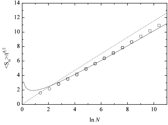
Figure 1: $\langle S_{N}(t)\rangle/t^{d_{s}/2}$ versus $\ln N$ in the two-dimensional incipient percolation aggregate. The lines represent the result of the zeroth-order approximation (dashed line) and the first-order approximation (solid line). The symbols are simulation results obtained with 40000 experiments for $t=1000$ (circles) and with 10000 experiments for $t=2000$ (squares).

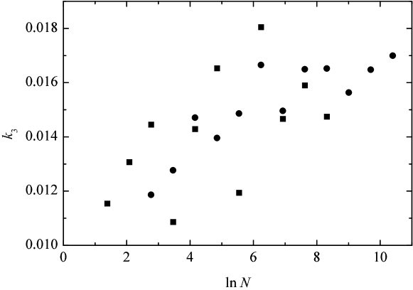
Figure 2: Simulation values of $k_{2}=\kappa_{2}(S_{N})/\langle S_{N}(t)\rangle^{2}$ versus $\ln N$ for the two-dimensional incipient percolation aggregate obtained averaging over $40000$ (squares) and 20000 (circles) experiments for $t=1000$.

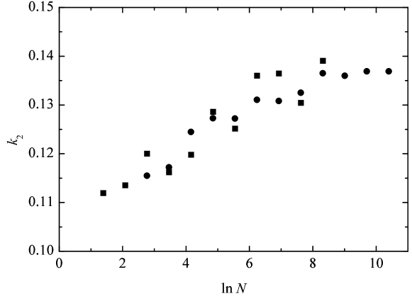
Figure 3: The same as Fig. 2 but for $k_{3}=\kappa_{3}(S_{N})/\langle S_{N}(t)\rangle^{3}$.

In our simulations we also evaluated the second cumulant (variance), $\kappa_{2}(S_{N})=\langle S_{N}^{2}\rangle-\langle S_{N}\rangle^{2}$, and the third cumulant, $\kappa_{3}(S_{N})=\langle S_{N}^{3}\rangle-3\langle S_{N}^{2}\rangle\langle S_{N}\rangle+2\langle S_{N}\rangle^{3}$, of the territory explored $S_{N}(t)$ as they are necessary for implementing the extended Rosenstock approximation (see Sec. IV). We found that the ratio $k_{m}\equiv\kappa_{m}(S_{N})/\langle S_{N}(t)\rangle^{m}$, although not very sensitive to the value of $N$ (one can see in Figs. 2 and 3 that these parameters are well represented by $k_{2}=0.13\pm 0.02$ and $k_{3}=0.015\pm 0.02$ over a wide range of $N$ values) seems to tend to a constant value for large $N$ (about $0.14$ for $k_{2}$ and $0.016$ for $k_{3}$). This is a surprising behavior that departs considerably from that of Euclidean media. For example, for the $d$-dimensional Euclidean lattices it was found that $k_{2}$ goes as $1/\ln^{2}N$ for large $N$. Also, the value of $k_{2}$ for large $N$ is much smaller than for the percolation aggregate (for example, for $N=2^{10}$, $k_{2}\simeq 1/15^{2},1/30^{2}$ and $1/50^{2}$ in the one-, two- and three-dimensional Euclidean lattices, respectively PREost ), which has important consequences for the accuracy of Rosenstock’s approximations of different orders, as we will show in Sec. IV. The disordered nature of the substrate must be the reason for these remarkable differences in the behavior of $k_{m}$. What is happening is that, for large $N$, the fluctuations in the number $S_{N}(t)$ of distinct sites explored by a large number $N$ of random walkers are dominated by the fluctuations (over the set of stochastic lattice realizations used in the simulations) of the number of sites inside a hypersphere of chemical radius $\ell=\sqrt{2D_{\ell}}\,t^{1/d_{w}^{\ell}}$. We summarize this claim in a conjecture as follows

$$\lim_{N\rightarrow\infty}k_{m}=\lim_{N\rightarrow\infty}\frac{\kappa_{m}(S_{N}(t))}{\langle S_{N}(t)\rangle^{m}}=\frac{\kappa_{m}(V)}{\langle V(\ell)\rangle^{m}}\equiv\ell_{m}\;,$$ (10)

where $V(\ell)$ is the chemical volume (number of sites) of a hypersphere of chemical radius $\ell$ and $\kappa_{m}(V)$ is the $m$th-cumulant of the distribution of $V$. Rigorously, the distance $\ell$ appearing in Eq. (10) is given by $\sqrt{2D_{\ell}}\,t^{1/d_{w}^{\ell}}$ which is the radius of the diffusion front in the thermodynamic limit ($N\rightarrow\infty$). However, the quotient $\ell_{m}$ is not very sensitive to $\ell$ if a sufficiently large value of $\ell$ is taken. In Fig. 4 we plot a histogram for the chemical volume of a two-dimensional incipient percolation aggregate with $\ell=100$, evaluated using $2000$ realizations of the lattice. Thereby we find that $\ell_{2}\simeq 0.14$ and $\ell_{3}\simeq 0.015$ in very good agreement with the values of $k_{2}$ and $k_{3}$, respectively, for large $N$ (see figures 2 and 3). Consequently, we conclude that the fluctuations in $S_{N}(t)$ are dominated by the disorder of the substrate and the influence of the value of $N$ is completely overshadowed. Similar arguments were presented by Rammal and Toulouse in their pioneer work on percolation clusters RT .

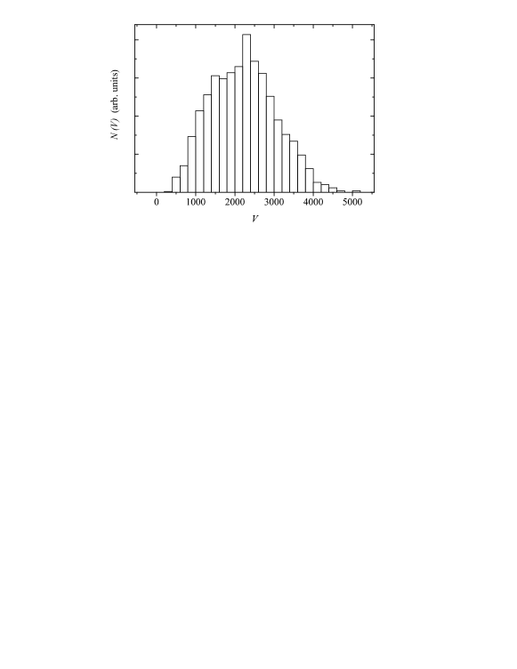
Figure 4: Histogram for the chemical volume inside a circle of chemical radius $\ell=100$ in the two-dimensional incipient percolation aggregate. A set of $2000$ randomly generated clusters in a $400\times 400$ square box were used in the computation. The distribution is clearly asymmetric around the maximum.

IV Order statistics of the trapping process

Assume that one has a quenched configuration of traps randomly placed on a given realization of the disordered lattice with probability $c$. If $N$ random walkers start from an origin site free from traps at $t=0$, it is clear that the probability that all random walkers survive by time $t$ is given by $(1-c)^{S_{N}(t)}$. The average of this quantity over all possible random walks, trap configurations, and substrate realizations is known as the survival probability: $\Phi_{N}(t)=\langle(1-c)^{S_{N}(t)}\rangle$. Using a well-known theorem in statistics, we can define the $n$th-order Rosenstock approximation $\Phi_{N}^{(n)}(t)$ for estimating $\Phi_{N}(t)$ as

$$\Phi_{N}^{(n)}(t)=\exp\left[\displaystyle\sum_{j=1}^{n+1}\frac{(-\lambda)^{j}}{j!}\kappa_{j}(S_{N})\right]$$ (11)

where $\lambda\equiv-\ln(1-c)$ and $\kappa_{j}(S_{N})$ is the $j$th-cumulant of the distribution of the territory explored. In the limit $n\rightarrow\infty$ we recover the exact result for $\Phi_{N}(t)$. In the case of the single particle ($N=1$) trapping problem, Eq. (11) is known as the extended Rosenstock approximation or truncated cumulant expansion Hughes ; Havlin ; Hollander ; BluKlafZumPRB ; ZumofenBlumen ; Weiss . Its generalization to the $N$ particle case was used in a one-dimensional trapping problem in Ref. OneSided .

In the previous section we showed that Monte Carlo simulations strongly suggest that $\kappa_{n}(S_{N})\simeq k_{n}\langle S_{N}(t)\rangle^{n}$ for large $N$, where $k_{n}$ are constants. [Notice that $\kappa_{1}(S_{N})=\langle S_{N}(t)\rangle$, so that $k_{1}=1$.] Therefore, inserting this result into Eq. (11), the $n$th-order Rosenstock approximation becomes

$$\Phi_{N}^{(n)}(t)\simeq\exp\left[\displaystyle\sum_{j=1}^{n+1}\frac{(-\lambda)^{j}}{j!}\,k_{j}\,\langle S_{N}\rangle^{j}\right]\;$$ (12)

or equivalently, by using Eq. (8),

$$\Phi_{N}^{(n)}(t)\simeq\exp\left[\displaystyle\sum_{j=1}^{n+1}\frac{(-\lambda)^{j}}{j!}\,k_{j}\,\bar{S}_{N}^{j}\,t^{jd_{s}/2}\right]\;.$$ (13)

We can now evaluate an approximation for the moments of the first trapping time, $\langle t_{1,N}^{m}\rangle$, by means of Eq. (6) assuming that the contribution of $\Phi_{N}(t)$ to $\langle t_{1,N}^{m}\rangle$ is negligible for those times for which $\Phi_{N}(t)$ and $\Phi_{N}^{(n)}(t)$ differ substantially. Therefore, the substitution of Eq. (13) into Eq. (6) yields

$$\langle t_{1,N}^{m}\rangle\simeq\langle t_{1,N}^{m}\rangle_{n}\equiv m\int_{0}^{\infty}t^{m-1}\exp\left[\displaystyle\sum_{j=1}^{n+1}\frac{(-\lambda)^{j}}{j!}k_{j}\bar{S}_{N}^{j}t^{jd_{s}/2}\right]dt\;.$$ (14)

Writing $v=\lambda\bar{S}_{N}t^{d_{s}/2}$, the $n$th-order Rosenstock’s estimate $\langle t_{1,N}^{m}\rangle_{n}$ for $\langle t_{1,N}^{m}\rangle$ becomes:

$$\langle t_{1,N}^{m}\rangle_{n}=\frac{2m}{d_{s}}\left(\lambda\bar{S}_{N}\right)^{-2m/d_{s}}\tau_{n}(m)$$ (15)

where

$$\tau_{n}(m)=\int_{0}^{\infty}v^{2m/d_{s}-1}\exp\left[\displaystyle\sum_{j=1}^{n+1}\frac{(-1)^{j}}{j!}k_{j}\,v^{j}\right]dv\;.$$ (16)

Therefore, we find that the different $n$th-order Rosentock approximations $\langle t_{1,N}^{m}\rangle_{n}$ differ from each other only by a numerical factor $\tau_{n}(m)$ (an integral) that depends only on the substrate through its spectral dimension $d_{s}$ and the set of parameters $k_{j}$, $j=1,2,\ldots$ that come from the distribution of the chemical volume of this substrate [c.f. Eq. (10)]. The integral in Eq. (16) is trivial for $n=0$ and yields $\tau_{0}(m)=\Gamma(2m/d_{s})$. Using the values of Table 1 we get $d_{s}=2d_{\ell}/d_{w}^{\ell}\simeq 1.375$ and the estimates $\tau_{0}(1)\simeq 0.89$, $\tau_{0}(2)\simeq 1.95$ and $\tau_{0}(3)\simeq 10.9$ for the two-dimensional incipient percolation aggregate. The integral in Eq. (16) only converges for even values of $n$ so the next meaningful approximation corresponds to $n=2$. Taking the values $k_{2}=0.13$ and $k_{3}=0.015$ (which describe $k_{2}$ and $k_{3}$ well over the range of values of $N$ used in our simulations: see Figs. 2 and 3) and evaluating the integral in Eq. (16) numerically, we found the second-order prefactors $\tau_{2}(m)$: $\tau_{2}(1)\approx 1.24$, $\tau_{2}(2)\approx 6.04$ and $\tau_{2}(3)\approx 95.6$, which are systematically much larger than the zeroth-order ones $\tau_{0}(m)$, especially when the order $m$ of the moment is large. This means that Rosenstock’s approximations of order higher than zero must be necessary to provide reasonable predictions for $\Phi_{N}(t)$ and $\langle t_{1,N}^{m}\rangle$ in disordered media, especially when the moment $m$ is large. It should be noticed that the expression for the first trapping time in Eq. (15) includes two approximations of different nature: (a) one due to the fact that we are using a finite number $n$ of terms in the cumulant expansion [which only affects the factor $\tau_{n}(m)$]; and (b) the other due to the finite number of terms considered for estimating $\bar{S}_{N}$ by means of the asymptotic series (9). Consequently, it is convenient to classify these approximations by indexing them with a pair of integers $(n,l)$: the first index gives the order of the Rosenstock approximation that is used, and the second gives the number of terms considered in the evaluation of $\langle S_{N}(t)\rangle$. In this way, the approximation $(n,0)$ corresponds to the replacement in Eq. (15) of $\bar{S}_{N}$ by the leading term of the series of Eq. (9), so that $\langle t_{1,N}^{m}\rangle_{n}=\langle t_{1,N}^{m}\rangle_{n0}[1+O(1/\ln N)]$ with

$$\langle t_{1,N}^{m}\rangle_{n0} = \frac{2m\tau_{n}(m)}{d_{s}\left[\lambda V_{0}(2D_{\ell})^{d_{\ell}/2}\right]^{2m/d_{s}}}\left(\frac{\ln N}{\hat{c}}\right)^{m(1-d_{w}^{\ell})}$$ (17)

$$= \frac{T_{n}(m)}{\lambda^{2m/d_{s}}(\ln N)^{m(d_{w}^{\ell}-1)}}\;,$$ (18)

and where we have absorbed all the dependence on the lattice characteristic parameters ($V_{0}$, $D_{\ell}$, $d_{s}$, …) into the coefficient $T_{n}(m)$. In the same way, if we take the two first terms in the asymptotic series of of Eq. (9), we find $\langle t_{1,N}^{m}\rangle_{n}=\langle t_{1,N}^{m}\rangle_{n1}[1+O(1/\ln N)^{2}]$ where the approximation $(n,1)$ is

$$\langle t_{1,N}^{m}\rangle_{n1}=\frac{T_{n}(m)}{\lambda^{2m/d_{s}}(\ln N)^{m(d_{w}^{\ell}-1)}}\left[1-d_{\ell}\frac{d_{w}^{\ell}-1}{d_{w}^{\ell}}\frac{s_{0}^{(1)}+s_{1}^{(1)}\ln N}{\ln N}\right]^{-2m/d_{s}}$$ (19)

or, for $\ln N\gg 1$,

$$\langle t_{1,N}^{m}\rangle_{n1}=\frac{T_{n}(m)}{\lambda^{2m/d_{s}}(\ln N)^{m(d_{w}^{\ell}-1)}}\left[1+m(d_{w}^{\ell}-1)\frac{s_{0}^{(1)}+s_{1}^{(1)}\ln N}{\ln N}\right]\;.$$ (20)

In Fig. (5) we compare simulation results for the trapping time of the first particle with the theoretical predictions given by Eqs. (18) and (19) when the parameters of Table 1 are used. We see that the second-order Rosenstock approximation leads to much better results than the standard zeroth-order approximation.

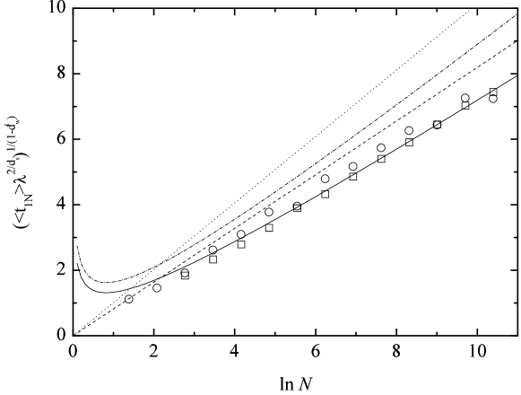
Figure 5: $\left(\langle t_{1,N}\rangle\lambda^{2/d_{s}}\right)^{1/(1-d_{w}^{\ell})}$ versus $\ln N$ for the two-dimensional incipient percolation aggregate. The lines represent the $n$th-order Rosenstock approximation that uses the $l$th-order approximation for $S_{N}(t)$ with, from top to bottom, $n=0$ and $l=0$ (dotted line), $n=0$ and $l=1$ (dashed-dotted line), $n=2$ and $l=0$ (dashed line), and $n=2$ and $l=1$ (solid line). In this and the following figures we have used $k_{2}=0.13$ and $k_{3}=0.015$. The symbols represent simulation results for $c=0.008$ (average over $2000$ lattice realizations; circles) and $c=0.001$ ($20000$ lattice realizations; squares).

The moments $\langle t_{j,N}^{m}\rangle$, $j=2,3,\ldots$ corresponding to the trapping of the $j$th particle absorbed by the traps can be easily estimated by means of Eq. (5). However, we can also obtain an explicit expression for $\langle t_{j,N}^{m}\rangle$ if we approximate the difference operator $\nabla^{j}$ in (5) by the derivative $d^{j}/dN^{j}$. The error in this approximation can be estimated from the equation

$$\frac{\nabla^{j}f(N)}{(\Delta N)^{j}}=\frac{d^{j}f(N)}{dN^{j}}+O\left(\frac{d^{j+1}f(N)}{dN^{j+1}}\,\Delta N\right).$$ (21)

In our case $f(N)$ is $\langle t_{1,N}^{m}\rangle$ and $\Delta N=1$ so that

$$\nabla^{j}\langle t_{1,N}^{m}\rangle=\frac{d^{j}\langle t_{1,N}^{m}\rangle}{dN^{j}}+O\left(\frac{d^{j+1}\langle t_{1,N}^{m}\rangle}{dN^{j+1}}\right).$$ (22)

As

$$\frac{d^{j}}{dN^{j}}(\ln N)^{-\mu}=(-1)^{j}\mu\frac{(j-1)!}{N^{j}}(\ln N)^{-\mu-1}+\frac{\ln\ln N}{N^{j}}{O}[(\ln N)^{-\mu-2}]$$ (23)

one finds, from Eq. (18) [or Eq.(19)], that

$$\nabla^{j}\langle t_{1,N}^{m}\rangle=\frac{d^{j}\langle t_{1,N}^{m}\rangle}{dN^{j}}\left[1+O(N^{-1})\right].$$ (24)

Taking into account that $\binom{N}{j}/N^{j}\simeq 1/j!$ for $j\ll N$, we obtain from Eqs.  (5), (18) [or (19)] and (23) the recursion relation

$$\langle t_{j+1,N}^{m}\rangle=\langle t_{j,N}^{m}\rangle+\frac{1}{j}m(d_{w}^{\ell}-1)T_{n}(m)\lambda^{-2m/d_{s}}(\ln N)^{-m(d_{w}^{\ell}-1)-1}\left[1+O\left(\frac{1}{\ln N}\right)\right]\;$$ (25)

which can be easily solved:

$$\langle t_{j,N}^{m}\rangle=\langle t_{1,N}^{m}\rangle+m(d_{w}^{\ell}-1)T_{n}(m)\lambda^{-2m/d_{s}}\frac{\psi(j)+\gamma}{(\ln N)^{m(d_{w}^{\ell}-1)+1}}\left[1+O\left(\frac{1}{\ln N}\right)\right]\;$$ (26)

where

$$\psi(j)=\psi(1)+\sum_{r=1}^{j-1}\frac{1}{r}$$ (27)

is the psi (digamma) function abramo , $\psi(1)=-\gamma$, and $\gamma$ is the Euler constant. Equation (26) yields

$$\langle t_{j,N}^{m}\rangle_{n0}=\frac{T_{n}(m)}{\lambda^{2m/d_{s}}(\ln N)^{m(d_{w}^{\ell}-1)}}$$ (28)

by using Eq. (18), and

$$\langle t_{j,N}^{m}\rangle_{n1}=\frac{T_{n}(m)}{\lambda^{2m/d_{s}}(\ln N)^{m(d_{w}^{\ell}-1)}}\left[1+m(d_{w}^{\ell}-1)\frac{\psi(j)+\gamma+s_{0}^{(1)}+s_{1}^{(1)}\ln N}{\ln N}\right]$$ (29)

when Eq. (20) is used. In Fig. (6) we compare the predictions for $\langle t_{2,N}\rangle$ obtained from Eqs. (28) and (29) with simulation results. The results are similar to that found in Fig. (5) for $\langle t_{1,N}\rangle$. In Fig. (7) the differences $\langle t_{j+1,N}\rangle-\langle t_{j,N}\rangle$ estimated from Eq. (25) are also plotted in a scaled form for $j=1,2$. The theoretical prediction is that, for large $N$, these points should tend to lie along a straight line (which is true) with a slope $(d_{w}^{\ell}-1)T_{2}(1)/j$, i.e., a slope $0.76$ for $j=1$ and 1.0 for $j=2$. The last prediction is not good for $j=2$ (the fitted value is 0.90), but this should not be surprising because in Eq. (25) we have ignored correction terms of order $1/\ln N$, which are very large even for huge values of $N$. The only way to remedy this deficiency would be by increasing the number of asymptotic terms retained in the evaluation of $\langle S_{N}(t)\rangle$, which in turns requires knowing $s_{m}^{(n)}$ for $n\geq 2$ [c.f. Eq. (9)]. Unfortunately, these values of $s_{m}^{(n)}$ are very difficult to estimate by means of numerical simulations SNtFrac and are unknown for $n\geq 2$.

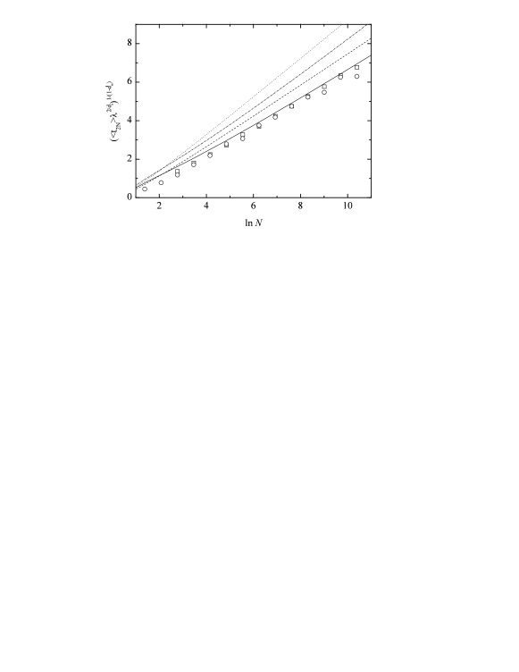
Figure 6: The same as Fig. 5 but for $\left(\langle t_{2,N}\rangle\lambda^{2/d_{s}}\right)^{1/(1-d_{w}^{\ell})}$.

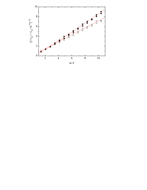
Figure 7: Simulation results of $\left[\left(\langle t_{j+1,N}\rangle-\langle t_{j,N}\rangle\right)\lambda^{2/d_{s}}\right]^{-1/d_{w}^{\ell}}$ when $j=1$ (hollow symbols) and $j=2$ (filled symbols) for the two-dimensional incipient percolation aggregate. Squares [circles] represent simulation results for $c=0.001$ [$c=0.008$] averaged over $20000$ [$2000$] lattice realizations. The lines are linear fits with slopes 0.72 (bottom) and 0.90 (top).

The variance of $t_{j,N}$ is easily obtained from Eq. (15):

$$\sigma_{j,N}^{2}=\frac{[T_{n}(2)-T_{n}^{2}(1)]}{\lambda^{4/d_{s}}(\ln N)^{2(d_{w}^{\ell}-1)}}\left[1+2(d_{w}^{\ell}-1)\frac{\psi(j)+\gamma+s_{0}^{(1)}+s_{1}^{(1)}\ln N}{\ln N}+O\left(\frac{1}{\ln^{2}N}\right)\right]\;$$ (30)

and, consequently,

$$\frac{\sigma_{j,N}^{2}}{\langle t_{1,N}\rangle^{2}}=d_{s}\frac{\tau_{n}(2)}{\tau_{n}(1)^{2}}-1\;.$$ (31)

This is an interesting result because it means that the ratio between the variance of the first trapping time and the mean of that time is, for large $N$, independent of $N$. The numerical value of the ratio $\sigma_{j,N}/\langle t_{1,N}\rangle$ is $[d_{s}\Gamma(4/d_{s})/\Gamma^{2}(2/d_{s})]-1\simeq 1.53$ for the zeroth-order Rosenstock approximation, and $2.0$ for the second-order approximation. In Fig. 8 we plot this ratio for $j=1,2,3$ versus $\ln N$, and the second-order theoretical limit $\sigma_{j,N}/\langle t_{1,N}\rangle\simeq 2$ seems to be consistent with the simulation data.

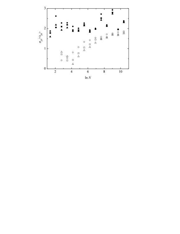
Figure 8: Simulation values of $\sigma_{j,N}/\langle t_{j,N}\rangle$ versus $\ln N$ for $j=1$ (circles), $j=2$ (squares) and $j=3$ (triangles) and two trap concentrations: $c=0.001$ (hollow symbols; $20000$ lattice realizations) and $c=0.008$ (filled symbols; $2000$ lattice realizations) for the two-dimensional incipient percolation aggregate. The second order Rosenstock approximation predicts a ratio close to $2$ for large values of $N$.

Some considerations about the range of validity of the approximations developed in this paper are called for at this point. The approximation for $\langle S_{N}(t)\rangle$ in Eqs. (8) and (9) is only valid in the so called Regime II or intermediate time regime SNtFrac ; MultiparticleReview . As the integral in Eq. (6) was evaluated assuming that the expression for $\langle S_{N}(t)\rangle$ was valid for all times we conclude that the integral of $mt^{m-1}\Phi_{N}(t)$ over the short-time interval $[0,t_{\times}]$ ($t_{\times}\sim\ln N$ being the crossover time between Regime I and Regime II) has to be negligible relative to $\langle t_{1,N}^{m}\rangle$, or equivalently $(\ln N)^{m}\ll\langle t_{1,N}^{m}\rangle$, for our approach and our results being reasonable. Taking into account the estimate for $\langle t_{1,N}^{m}\rangle$ given in Eq. (18), this condition can be written as $\lambda\ll(\ln N)^{-d_{\ell}}$. The concentrations of traps we have used in our simulations, $c=0.001$ and $c=0.008$, verify this condition for all the values of $N$ considered. Apart from this upper bound on $c$, we must also point out that, as also for Euclidean lattices, our results break down if most of the trapping takes place within the long-time Donsker-Varadhan regime DV . Further reference to this limitation of the theory presented in this paper will be made below.

V Summary and conclusions

We have dealt with the following order statistics problem: when $N$ independent random walkers all starting from the same site diffuse on a disordered lattice populated with a concentration $c$ of static trapping sites, what is the distribution of the elapsed times, $t_{j,N}$, until the first $j$ random walkers are trapped? We were able to generalize the theory developed for the special case of Euclidean lattices PREost to the case of disordered substrates, and asymptotic expressions for the moments $\langle t_{j,N}^{m}\rangle$ with $j\ll N$ were obtained. To this end, we used the so-called Rosenstock approximation, which is suitable for not very large times and small concentrations of traps, $c$. In this approximation the survival probability of the full set of $N$ random walkers, $\Phi_{N}(t)$, is expressed in terms of the cumulants $\kappa(S_{N})$ of the distribution of the territory covered $S_{N}(t)$.

Monte Carlo simulation results for $\kappa(S_{N})$ in the two-dimensional incipient percolation aggregate showed that for large $N$ the ratio $k_{m}=\kappa_{m}(S_{N})/\langle S_{N}(t)\rangle^{m}$ with $m=2,3$ hardly depends on $N$ and is very large in comparison with the corresponding Euclidean ratio. We attribute this behavior to the fluctuations in $S_{N}(t)$ being dominated by the fluctuations in the volume of the medium inside a hypersphere of chemical radius $\ell\sim\sqrt{2D_{\ell}}\,t^{1/d_{w}^{\ell}}$. This claim is supported by the result $k_{m}\approx l_{m}$ for $N\gg 1$ found by simulations of $S_{N}(t)$ and $V(\ell)$ in two-dimensional incipient percolation aggregates, where $l_{m}=\kappa_{m}(V)/\langle V(\ell)\rangle^{m}$ characterizes the fluctuations in the volume $V(\ell)$. Therefore, the result $k_{m}\approx l_{m}$ for $N\gg 1$ implies that the fluctuations in $S_{N}(t)$ are mainly accounted for by the fluctuations in $V(\ell)$, and that the fluctuations in $S_{N}(t)$ induced by the randomness of the diffusion process are irrelevant. One expects this also to be true for other disordered media. Hence, if $\langle S_{n}(t)\rangle$ is known, the cumulants of the distribution of $S_{N}(t)$ can be calculated (for any sufficiently large value of $N$) from the cumulants of the distribution of the chemical volume. Finally, taking into account that $\langle S_{N}(t)\rangle$ is reasonably well known SNtFrac , we arrive at a closed expression for the survival probability $\Phi_{N}(t)$ [c.f. Eq. (12)] using Rosenstock’s approximation. But from $\Phi_{N}(t)$ one gets the probability $\Phi_{jN}(t)$ that $j$ random walkers of the initial set of $N$ have been absorbed by time $t$ [c.f. Eq. (2)], so that, finally, we get the moments of the trapping times, $\langle t_{j,N}^{m}\rangle$ from the first moment $\langle S_{n}(t)\rangle$ of the territory explored!

Comparison with simulation data shows that, in contrast with the Euclidean case, Rosenstock’s approximations of order higher than zero are necessary to account for the order statistics results in the two-dimensional percolation aggregate. This is a consequence of the large value (in comparison with the Euclidean case) of $k_{m}$, due to the large fluctuations in the territory explored by the random walkers, induced, as we showed, by the spatial disorder of the substrate. However, some features of the order statistics of trapping hold in the disordered case: for example, we found that the ratio $\sigma_{j,N}/\langle t_{j,N}\rangle$ depends only on the lattice characteristic parameters $d_{s}$ and $k_{m}$, $m=1,2,\ldots$ for large $N$. This was confirmed by simulations in two-dimensional percolation aggregates.

There are some interesting problems that we still cannot answer with the theory developed in this paper. For example, an important quantity is the time $t_{N,N}$ elapsed until all the particles of the inital set of $N$ are trapped. The evaluation of the moments of this quantity would require specific techniques for $j\approx N$ as our results are limited to the opposite limit $j\ll N$. Moreover, the trapping of the last particles surely takes place in the Donsker-Varadhan time regime DV where Rosenstock’s approximation for the survival probability cannot be used. The recent development of a Monte Carlo method to evaluate confidently the survival probability in the Donsker-Varadhan time regime for Euclidean lattices by Barkema et al.  Barkema following a previous work of Gallos et al.  Gallos could serve as starting point for tackling this problem. However, one should be aware that this task is not a straightforward generalization to disordered media of that carried out for Euclidean lattices because one has to take into consideration that, as Shapir Shapir pointed out, the Donsker-Varandhan long-time behavior is dominated by the subset of lattice realizations that are more ramified (with $d_{s}=1$). Consequently, an efficient Monte Carlo technique to explore the relevant rare lattice realizations in percolation clusters has to be devised before.

- (1) J. R. Beeler, Phys. Rev. 134, 1396 (1964); E. W. Montroll, J. Phys. Soc. Jap. Suppl. 26, 6 (1969); E. W. Montroll, J. Math. Phys. 10, 753 (1969); J. K. Anlauf, Phys. Rev. Lett. 52 1845 (1984).
- (2) A. Blumen, J. Klafter and G. Zumofen, Optical Spectroscopy of Glasses, edited by I. Zschokke (Reidel, Dordrecht, 1986).
- (3) B. H. Hughes, Random Walks and Random Environments (Clarendon Press, Oxford, 1995), Vol. 1; Random Walks and Random Environments (Clarendon Press, Oxford, 1995), Vol. 2.
- (4) S. Havlin and D. Ben-Avraham, Adv. Phys. 36, 695 (1987).
- (5) F. den Hollander and G. H. Weiss, Contemporary Problems in Statistical Physics, edited by G. H. Weiss (SIAM, Philadelphia, 1994), pp. 147-203.
- (6) J. R. Beeler, Phys. Rev. 134, 1396 (1964).
- (7) H. B. Rosenstock, Phys. Rev. 187, 1166 (1969).
- (8) P. Damask and P. Dienes, Point Defects in Metals (Gordon and Breach, New York, 1964).
- (9) G. Oshanin, S. Nechaev, A. M. Cazabat and M. Moreau Phys. Rev. E 58, 6134 (1998); S. Nechaev, G. Oshanin and A. Blumen, J. Stat. Phys. 98, 281 (2000).
- (10) H. Miyagawa, Y. Hiwatari, B. Bernu and J. P. Hansen, J. Chem. Phys. 88, 3879 (1988); T. Odagaki, J. Matsui and Y. Hiwatari, Phys. Rev. E 49, 3150 (1994).
- (11) P. L. Krapivsky and S. Redner, J. Phys. A 29, 5347 (1996); S. Redner and P. L. Krapivsky, Am. J. Phys. 67, 1277 (1999).
- (12) S. B. Yuste and L. Acedo, Physica A 297, 321 (2001).
- (13) S. B. Yuste and L. Acedo, Phys. Rev. E 64, 061107 (2001).
- (14) For reviews, see T. Bache, W. E. Moerner, M. Orrit, and U. P. Wild, Single-Molecule Optical Detection, Imaging and Spectroscopy (VCH, Weinheim, 1996); X. S. Xie and J. K. Trautman, Annu. Rev. Phys. Chem. 49, 441 (1998). See also the section “Single Molecules” in Science 283, 1667 (1999).
- (15) M. T. Valentine, P. D. Kaplan, D. Thota, J. C. Crocker, T. Gisler, R. K. Prud’homme, M. Beck and D. A. Weitz, Phys. Rev. E 64, 061506 (2001).
- (16) Fractals in Science, edited by A. Bunde and S. Havlin (Springer-Verlag, Berlin, 1994); Fractals and Disordered Systems, edited by A. Bunde and S. Havlin (Springer-Verlag, Berlin, 1996).
- (17) P. Pfeifer, F. Ehrburger-Dolle, T. P. Rieker, M. T. González, W. P. Hoffman, M. Molina-Sabio, F. Rodríguez-Reinoso, P. W. Schmidt and D. J. Voss, Phys. Rev. Lett. 88, 115502 (2002).
- (18) A. Blumen, J. Klafter and G. Zumofen, Phys. Rev. B 28, 6112 (1983).
- (19) H. Larralde, P. Trunfio, S. Havlin, H. E. Stanley and G. H. Weiss, Phys. Rev. A 45, 7128 (1992).
- (20) L. Acedo and S. B. Yuste, Phys. Rev. E 63, 011105 (2001); cond-mat/0003446.
- (21) K. Lindenberg, V. Seshadri, K. E. Shuler and G. H. Weiss, J. Stat. Phys. 23, 11 (1980).
- (22) G. H. Weiss, K. E. Shuler and K. Lindenberg, J. Stat. Phys. 31, 255 (1983).
- (23) S. B. Yuste and K. Lindenberg, J. Stat. Phys. 85, 501 (1996); S. B. Yuste, Phys. Rev. Lett. 79, 3565 (1997); Phys. Rev. E 57, 6327 (1998); S. B. Yuste and L. Acedo, J. Phys. A 33, 507 (2000); S. B. Yuste, L. Acedo and K. Lindenberg, Phys. Rev. E 64, 052102 (2001).
- (24) J. Dräger and J. Klafter, Phys. Rev. E 60, 6503 (1999).
- (25) O. Benichou, M. Coppey, J. Klafter, M. Moreau and G. Oshanin, J. Phys. A 36, 7225 (2003).
- (26) P. G. de Gennes, La Recherche 7, 919 (1976).
- (27) H. Larralde, P. Trunfio, S. Havlin, H. E. Stanley and G. H. Weiss, Nature (London) 355, 423 (1992); G. H. Weiss, I. Dayan, S. Havlin, J. E. Kiefer, H. Larralde, H. E. Stanley and P. Trunfio, Physica A 191, 479 (1992); A. M. Berezhkovskii, J. Stat. Phys. 76, 1089 (1994); G. M. Sastry and N. Agmon, J. Chem. Phys. 104, 3022 (1996).
- (28) S. B. Yuste and L. Acedo, Phys. Rev. E 60, R3459 (1999); 61, 2340 (2000).
- (29) L. Acedo and S. B. Yuste, in Recent Research Developments in Statistical Physics, Vol. 2, (Transworld Research Network, Trivandrum, 2002).
- (30) R. Rammal and G. Toulouse, J. Physique Lett. 44, (1983).
- (31) G. Zumofen and A. Blumen, Chem. Phys. Lett. 83, 372 (1981).
- (32) G. H. Weiss, Aspects and Applications of the Random Walk (North-Holland, Amsterdam, 1994).
- (33) Handbook of Mathematical Functions, edited by M. Abramowitz and I. Stegun (Dover, New York, 1972).
- (34) D.V. Donsker and S. R. S. Varadhan, Commun. Pure Appl. Math. 28, 525 (1975); A. A. Ovchinnikov and Y. B. Zeldovich, Chem. Phys. 28, 215 (1978); P. Grassberger and I. Procaccia, J. Chem. Phys. 77, 6281 (1982); R. F. Kayser and J. B. Hubbard, Phys. Rev. Lett. 51, 79 (1983).
- (35) G.T. Barkema, P. Biswas and H. van Beijeren, Phys. Rev. Lett. 87, 170601 (2001).
- (36) L. K. Gallos, P. Argyrakis and K. W. Kehr, Phys. Rev. E. 63, 021104 (2001).
- (37) Y. Shapir, J. Physique Lett. 45, L-895 (1984).