Extraction of domain-specific magnetization reversal for nanofabricated periodic arrays using soft x-ray resonant magnetic scattering

Abstract

A simple scheme to extract the magnetization reversals of characteristic magnetic domains on nanofabricated periodic arrays from soft x-ray resonant magnetic scattering (SXRMS) data is presented. The SXRMS peak intensities from a permalloy square ring array were measured with field cycling using circularly polarized soft x-rays at the Ni L₃ absorption edge. Various SXRMS hysteresis loops observed at different diffraction orders enabled the determination of the magnetization reversal of each magnetic domain using a simple linear algebra. The extracted domain-specific hysteresis loops reveal that the magnetization of the domain parallel to the field is strongly pinned, while that of the perpendicular domain rotates continuously.

Understanding the reversal mechanism of the magnetization in periodic arrays of submicron and nanoscale magnets is of both scientific and technological interest. Fundamental changes in the statics and the dynamics of magnetization reversal imposed by nanostructures enrich the physics of nanomagnetism. A precise control of magnetization reversal involving well-defined and reproducible magnetic domain states in nanomagnet arrays is key to future applications, such as high density magnetic recordingrecord_jpd_02 or magnetoelectronicspintronics_ieee_03 devices. To achieve this, topologically various nanomagnets, ranging from simple disksdisk_jpd_00 to more complicated ringsring_prl_01 or negative dots (holes)hole_apl_97 , have been investigated. However, as rather well-defined but non-single magnetic domains (or domain states) form in complicated geometries, it becomes difficult to characterize precisely magnetization reversal involving each domain at small-length scales with either conventional magnetization loop measurements, such as magneto-optical Kerr effect (MOKE) magnetometry, or magnetic microscopy, such as magnetic force microscopy (MFM). Moreover, in large-area arrays typically covering areas of a few square millimeters, extracting overall domain structures during reversal from microscopic images is clearly unreliable. Though diffracted MOKE measurement has been proposed recently to deal with this problem, it is found to provide little quantitative information on magnetization reversal involving domain formation and is limited to micrometer-length scales.dmoke_prb_02

Such quantitative information is available using the technique of soft x-ray resonant magnetic scattering (SXRMS).kao_prl_90 This technique exploits strong enhancement of the magnetic sensitivity of scattering intensities when incident circularly polarized soft x-rays are tuned to an absorption edge of constituent magnetic atoms. SXRMS has been used to study the magnetic structure in magnetic thin filmssxrms_film or periodic arrays of stripe domains or nanolinessxrms_line . In this paper we present a simple scheme to extract quantitatively domain-specific magnetization reversal for nanomagnet arrays from SXRMS measurements. For this purpose, sample rocking curves, yielding in-plane diffraction scans, have been measured and analyzed on the basis of our previous work performed in the hard x-rays.lee_dot In order to obtain magnetic information, SXRMS peak intensities were measured by varying the applied field at different diffraction orders, whose scattering structure factors are different. This allows us to determine directly the magnetization reversal of each magnetic domain using a simple linear algebra. The basic idea of incorporating such nonuniform magnetic domains in scattering theory has been explored in our previous work on polarized neutron scattering.lee_neutron

For this study an array of permalloy (Ni₈₀Fe₂₀) square rings was fabricated by a combination of e-beam lithography and lift-off techniques. A standard silicon wafer was spin-coated with a double-layer positive-type e-beam resist, and the resist layer was then patterned by e-beam lithography. A 20-nm-thick permalloy film was deposited onto it using an electron-beam evaporator in a vacuum of about $10^{-8}$ Torr. The as-deposited unpatterned film was magnetically soft with coercive and uniaxial anisotropy fields of a few Oersteds. Finally, after ultrasonic-assisted lift-off, the square rings were arranged in an array of 2 $\times$ 2 mm².

Experiments were performed at sector 4 of the Advanced Photon Source.sector4 Polarized soft x-rays at the beamline 4-ID-C were generated by a novel circularly polarized undulator that provided left- and right-circular polarization switchable on demand at a polarization $>96$%. The photon energy was tuned to the Ni L₃ absorption edge (853 eV) to enhance the magnetic sensitivity. While a vacuum compatible sample stage was rotated, the diffracted soft x-ray intensities were collected by a Si photodiode detector with a fixed angle of 12.8^∘. This sample rocking scan, where the incident and exit angles $\theta_{i}$ and $\theta_{f}$ were varied with the total scattering angle $(\theta_{i}+\theta_{f})$ fixed, yielded a transverse $q_{x}$ scan at a fixed $q_{z}$ value (see Fig. 1). The angular resolution was defined by a pinhole between the sample and detector to be about 0.03^∘. The sample was mounted in the gap of an eletromagnet that provides fields in the scattering plane of up to $\pm 800$ Oe.

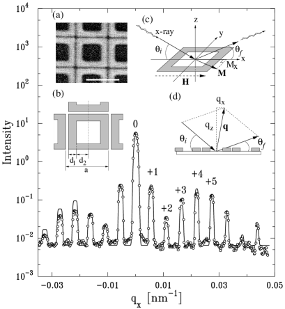
Figure 1: Diffraction intensities of the rocking scan along the $q_{x}$ direction at $q_{z}=0.955$ ${\rm nm}^{-1}$ from a square ring array. Circularly polarized soft x-rays were used and the photon energy was tuned to the Ni L₃ absorption edge (853 eV). Circles represent measurements, and lines represent the calculations. Insets: (a) scanning electron micrograph and (b) schematic of the square ring array studied. The scale bar is 1 $\mu$m. (c) and (d) show schematics of the scattering geometry, where $\theta_{i}$ and $\theta_{f}$ are the incidence and exit angles, and ${\bf H}$ and ${\bf M}$ are the applied field and magnetization, respectively.

Figure 1 shows the diffraction intensities of the sample rocking scan measured as a function of $q_{x}$ at $q_{z}=0.955$ nm^-1 from the square ring array with the saturation field. Diffracted intensities show peaks corresponding to an array period of 1.151 $\mu$m. Following Refs. lee_dot, ; lee_neutron, , the diffracted intensity $I$ can be expressed in the kinematical approximation as

$$I(q_{x};H) = |F(q_{z})|^{2}\sum_{n_{x},|n_{y}|}\Bigl{|}\rho_{C}F_{C}\bigl{(}n_{x},|n_{y}|\bigr{)}$$ (1)

$$+ \rho_{M}F_{M}\bigl{(}n_{x},|n_{y}|;H\bigr{)}\Bigr{|}^{2}{\cal R}\bigl{(}q_{x};n_{x},|n_{y}|\bigr{)},$$

where $H$ is the applied field, $F(q_{z})$ is the 1D form factor along $q_{z}$ direction and consequently a constant value for a fixed $q_{z}$, and $F_{C(M)}$ and $\rho_{C(M)}$ are the charge (magnetic) form factors on the $q_{x}-q_{y}$ plane and the charge (magnetic) contributions to the total atomic scattering amplitude, respectively. Near resonance energies $\rho_{M}$ is proportional to the vector product $({\bf\hat{e}}^{\ast}_{f}\times{\bf\hat{e}}_{i})\cdot{\bf M}$,kao_prl_90 where ${\bf\hat{e}}_{i}$ and ${\bf\hat{e}}_{f}$ are unit photon polarization vectors for incident and scattered waves, respectively, and ${\bf M}$ is the magnetization vector. For circularly polarized beams, this vector product reduces approximately to the component $M_{x}$ in the inset (c) of Fig. 1. Therefore, the magnetization referred to hereafter represents strictly the parallel component to the $x$-axis or the field direction ($H\parallel\hat{x}$ in this study) of the magnetization vector. $n_{x}$, $n_{y}$ are indices for Bragg points in the reciprocal space with the relationship of $q_{x,y}=(2\pi/a)n_{x,y}$, where $a$ is the period of the array. Since the resolution function ${\cal R}$ is a long thin ellipse oriented in the $q_{y}$ direction, nonzero $n_{y}$ values should also be taken into account for a $q_{x}$-scan performed at $q_{y}=0$.lee_neutron ; lee_dot We also note that the evolution of the peak widths of the different diffracted orders as a function of $q_{x}$, as shown in Fig. 1, was calculated using the model proposed by Gibaud $et$ $al.$gibaud_jphy_96

For a square ring, the charge form factor $F_{C}(n_{x},|n_{y}|)$ can be expressed by

$$F_{C}\bigl{(}n_{x},|n_{y}|\bigr{)} = {\cal C}\biggl{[}{\rm sinc}\Bigl{(}n_{x}(\gamma_{1}+\gamma_{2})\Bigr{)}{\rm sinc}\Bigl{(}|n_{y}|(\gamma_{1}+\gamma_{2})\Bigr{)}$$ (2)

$$- \frac{\gamma_{2}^{2}}{(\gamma_{1}+\gamma_{2})^{2}}{\rm sinc}(n_{x}\gamma_{2}){\rm sinc}\Bigl{(}|n_{y}|\gamma_{2}\Bigr{)}\biggr{]},$$

where ${\cal C}$ is 1 for $|n_{y}|=0$ and 2 for $|n_{y}|\neq 0$, and ${\rm sinc}(x)=\sin(x)/x$. $\gamma_{1,2}=2\pi d_{1,2}/a$, where $d_{1}$ and $d_{2}$ are the width of the ring and half of the inner square size, respectively, as shown in inset (b) of Fig. 1. Since $F_{C}$ and $F_{M}$ are the same functional forms for a saturated uniform magnetization, the diffracted intensities can be calculated using Eqs. (1) and (2) and are shown as the solid line in Fig. 1. From the best fit, $d_{1}$ and $d_{2}$ were estimated to be $162\pm 4$ and $377\pm 4$ nm, respectively, and subsequently the gap between rings was 73 nm.

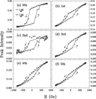
Figure 2: SXRMS magnetic hysteresis loops (circles) measured at several diffraction peaks, indicated by numbers in Fig. 1. The solid lines represent the calculated hysteresis loops.

Figure 2 shows SXMRS peak intensities measured at various diffraction orders while field cycling. All field dependencies show magnetic hysteresis loops but with different features. This is due to different magnetic form factors for different diffraction orders, which reflect nonuniform domain formation during magnetization reversal, as pointed out in diffracted MOKE studies.dmoke_prb_02 Therefore, the magnetic form factor $F_{M}$ in Eq. (1) should be expressed by the sum of the contributions of all possible magnetic domains, i.e.,

$$F_{M}\bigl{(}n_{x},|n_{y}|;H\bigr{)}=\sum_{l}m_{l}(H)F^{(l)}_{M}(n_{x},|n_{y}|),$$ (3)

where $m_{l}(H)$ represents the field-dependent magnetization of the $l$-th domain, which is the quantity of interest. It is noticeable that the magnetic factor in Eq. (3) can be factorized into the field- and structure-dependent factors. However, the domain-specific magnetization $m_{l}(H)$ cannot be directly extracted from measured SXRMS hysteresis loops because, as described in Eq. (1), the diffracted intensities are the absolute square of the sum of the structural and magnetic contributions.

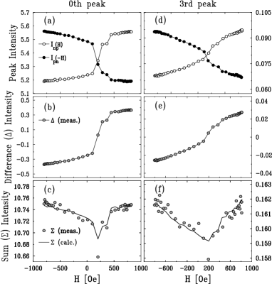
Figure 3: (a) and (d) SXRMS hysteresis loops with positive-to-negative intensities ($I_{pn}$) flipped with respect to $H=0$ for zeroth- and third-order peaks, respectively. Difference [(b) and (e)] and sum [(c) and (f)] intensities between $I_{np}(H)$ (negative-to-positive) and flipped $I_{pn}(-H)$ intensities as a function of the applied field. The solid lines in (c) and (f) represent the calculations.

To tackle this problem, we considered the difference between the field-dependent intensities of $I_{np}(H)$ and $I_{pn}(-H)$, where $I_{np}$, $I_{pn}$ represent the intensities measured while the field is swept along the negative-to-positive and positive-to-negative directions, respectively, and $I_{pn}(-H)$ represents the intensities flipped from $I_{pn}(H)$ with respect to $H=0$, as shown in Fig. 3. Assuming that the magnetization reversal has inversion symmetry about the origin, only the difference between $I_{np}(H)$ and $I_{pn}(-H)$ is the opposite sign of $m_{l}(H)$ in Eq. (3). However, this does not mean that they are symmetrical to a certain horizontal line in Fig. 3 (a) or (d) because the intensities contain quadratic terms to the magnetization $m_{l}(H)$, as described in Eq. (1), consequently leading to a nonsymmetry to the origin (or the center of mass) of SXRMS hysteresis loops in Fig. 2. This effect is clearly seen in the sum intensities of Figs. 3 (c) and (f) and will be an important characteristic of scattering-based hysteresis loops. However, in turn, these quadratic terms can be ruled out by taking the difference intensities, which are, as a result, linearly proportional to the magnetization.

These difference intensities at the $n_{x}$-order peak can be expressed from Eqs. (1) and (3) as

$$\Delta_{n_{x}}(H)\equiv I_{np}(n_{x};H)-I_{pn}(n_{x};-H)$$ (4)

$$~{}~{}~{}~{}~{}~{}~{}~{}~{}~{}~{}=4{\rm Re}[\rho_{C}\rho_{M}^{\ast}]{\cal R}_{n_{x}}|F(q_{z})|^{2}$$

$$~{}~{}~{}~{}\times\sum_{l}m_{l}(H)\sum_{|n_{y}|=0}^{\infty}F_{C}\bigl{(}n_{x},|n_{y}|\bigr{)}F_{M}^{(l)}\bigl{(}n_{x},|n_{y}|\bigr{)}{\cal R}_{n_{y}},$$

where ${\cal R}_{n_{x}}$ and ${\cal R}_{n_{y}}$ represent resolution functions evolving $n_{x}$ and $n_{y}$ indices, respectively, into which ${\cal R}(n_{x},|n_{y}|)$ in Eq. (1) can be factorized. If we further normalize $\Delta_{n_{x}}$ by its maximum intensity with a saturation magnetization $m_{s}$, we can obtain a set of linear equations as

$$\frac{\Delta_{n_{x}}(H)}{|\Delta_{n_{x}}^{\rm max}|}=\sum_{l}B_{n_{x}l}\frac{m_{l}(H)}{m_{s}},$$ (5)

where

$$B_{n_{x}l}=\frac{\sum_{|n_{y}|}F_{C}\bigl{(}n_{x},|n_{y}|\bigr{)}F_{M}^{(l)}\bigl{(}n_{x},|n_{y}|\bigr{)}{\cal R}_{n_{y}}}{\sum_{|n_{y}|}F_{C}^{2}\bigl{(}n_{x},|n_{y}|\bigr{)}{\cal R}_{n_{y}}}.$$ (6)

Here we used the relationship of $\sum_{l}^{all}F_{M}^{(l)}\bigl{(}n_{x},|n_{y}|\bigr{)}=F_{C}\bigl{(}n_{x},|n_{y}|\bigr{)}$. Applying linear algebra, the normalized magnetizations $m_{l=1,\cdot\cdot\cdot,N}(H)/m_{s}$ of $N$ domains can be finally obtained directly from the normalized difference intensities $\Delta_{n_{x}}(H)/|\Delta_{n_{x}}^{\rm max}|$ measured at $N$ different $n_{x}$ orders by taking the inverse of $N\times N$ matrix $B_{n_{x}l}$.

In principle, the field-dependent intensities measured at semi-infinite numbers of orders can thus be used to determine the magnetization reversal of each infinitesimal cell in a unit nanomagnet. However, this is practically restricted due to finite measurable diffraction peaks and a high symmetry of experimental geometry. The latter gives rise to a strong dependence between $F_{M}^{(l)}\bigl{(}n_{x},|n_{y}|\bigr{)}$ with different domain $l$ or diffraction order $n_{x}$, and, as a result, makes the matrix $B_{n_{x}l}$ singular and noninvertible. To lower the geometrical symmetry of experimental configuration, we can use a vector magnetometry setup by rotating the sample/electromagnet assembly with respect to the incident photon direction.lee_hole Since SXRMS intensities are proportional to the component of the magnetization vector along the projected incident photon direction onto the sample surface, this approach can also provide vectorial information about domain-specific magnetization.

In our setup, where both incident beam and field directions are parallel to one of the sides of the square rings, there may be four characteristic domains, as shown in the insets of Fig. 4. Each domain consists of two or four subdomains, whose structure-dependent form factors in Eq. (3) are identical, and, therefore, its magnetization represents an average value over subdomains. The explicit expressions of the structure-dependent magnetic form factors $F_{M}^{(l)}$ of these four domains for $(n_{x},|n_{y}|)$ diffraction order in Eq. (3) will be presented elsewhere.lee_elsewhere We note that these domains have been chosen to minimize sigularity of the matrix $B_{n_{x}l}$ and may not be thus energetically viable. Nevertheless, this scheme can unambiguously provide information about domain formation by considering snapshots of the resultant domain-specific magnetizations at each field.

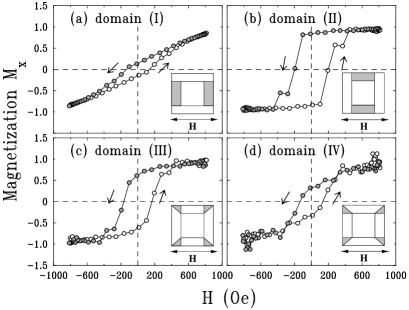
Figure 4: Extracted magnetization reversals along the field direction of four types of characteristic domains, which are depicted as gray-filled regions in the insets, from SXRMS hysteresis loops at zeroth-, first-, third-, and fifth-order peaks.

To construct a $4\times 4$ matrix $B_{n_{x}l}$ for four magnetic domains, at least four different peak intensities are required, and fifteen combinations can be allowed for six measured peaks, as shown in Fig. 2. However, we excluded the second peak due to its bad statistics and also some other combinations due to relatively small values of the determinants of their matrices $B_{n_{x}l}$, leading to a singularity of the matrix. For the optimum combination for non-singularity, zeroth-, first-, third-, and fifth-order peaks were then chosen. Figure 4 shows the finally extracted magnetization reversals for each domain using Eqs. (5) and (6). All magnetizations in Fig. 4 are normalized by the saturation and represent the components projected along the field direction, as discussed above, of the magnetization vectors. To confirm these results, the sum intensities in Figs. 3(c) and 3(f) and the SXMRS hysteresis loops for all observed peaks in Fig. 2 were also generated by substituting the results in Fig. 4 into Eq. (1). These calculations (solid lines) show a good agreement with the measurements.

A remarkable feature in the extracted magnetization reversals is that while the domain (I) perpendicular to the field rotates coherently, the parallel domain (II) is strongly pinned. Interestingly, this is similar to the domain behaviors in the antidot arrays,hole_apl_97 ; lee_hole whose geometry resembles the square ring array except for narrow gaps between rings. On the other hand, the domain (II) clearly shows plateaus, which have been observed generally in circular or octagonal ring magnets and are attributed to the vortex state.ring_prl_01 A detailed discussion is beyond the scope of this paper and will be presented elsewhere.lee_elsewhere

In summary, we successfully demonstrated that domain-specific magnetization reversals can be extracted directly from SXRMS hysteresis loops measured at various diffraction orders. Extracted domain-specific magnetization reversals are expected to provide a new insight into magnetic switching mechanism on nanofabricated arrays. Future studies, exploiting the element-selectivity and vector magnetometry setup, will provide further three-dimensional information in nanofabricated multilayers such as giant magnetoresistance and pseudospin valve structures.

Work at Argonne is supported by the U.S. DOE, Office of Science, under Contract No. W-31-109-ENG-38. V.M. is supported by the U.S. NSF, Grant No. ECS-0202780.

References

- (1) A. Moser et al., J. Phys. D: Appl. Phys. 35 R157 (2002).
- (2) S. Parkin et al., P. IEEE 91, 661 (2003).
- (3) R. P. Cowburn, J. Phys. D: Appl. Phys. 33 R1 (2000).
- (4) J. Rothman et al., Phys. Rev. Lett. 86, 1098 (2001); S. P. Li et al., ibid. 86, 1102 (2001).
- (5) R. P. Cowburn, A. O. Adeyeye, and J. A. C. Bland, Appl. Phys. Lett. 70, 2309 (1997).
- (6) I. Guedes et al., Phys. Rev. B66, 014434 (2002).
- (7) C. Kao et al., Phys. Rev. Lett. 65, 373 (1990).
- (8) J. M. Tonnerre et al., Phys. Rev. Lett. 75, 740 (1995); J. F. MacKay et al., ibid. 77, 3925 (1996); Y. U. Idzerda, V. Chakarian, and J. W. Freeland, ibid. 82, 1562 (1999); J. W. Freeland et al., Phys. Rev. B60, R9923 (1999); J. B. Kortright et al., ibid. 64, 092401 (2001).
- (9) H. A. Dürr et al., Science 284, 2166 (1999); K. Chesnel et al., Phys. Rev. B66, 024435 (2002).
- (10) D. R. Lee et al., Appl. Phys. Lett. 82, 982 (2003).
- (11) D. R. Lee et al., Appl. Phys. Lett. 82, 82 (2003).
- (12) J. W. Freeland et al., Rev. Sci. Instrum. 73, 1408 (2001).
- (13) A. Gibaud et al., J. Phys. I 6, 1085 (1996).
- (14) D. R. Lee et al., Appl. Phys. Lett. 81, 4997 (2002).
- (15) D. R. Lee et al., in preparation.