1. Introduction

Time-dependent or radiation induced phenomena in various mesoscopic electron systems has attracted considerable interest over the past few years [1, 2, 3, 4, 5]. These high-frequency modulated nanostructures, formed in a two-dimensional electron gas (2DEG) by applying appropriate confinement, are important both in connection with device application and can function as convenient samples to probe the properties of electron systems in reduced dimensions.

It is well discovered, in both theory [6] and experiment [7], that a quantum ring in a perpendicular magnetic field or an Aharonov-Bohm magnetic flux can carry an equilibrium current, the persistent current. This current is periodic in the magnetic flux enclosed by the ring with a period of the elementary flux quantum $\Phi_{0}=hc/e$. We present here a method to change the persistent current pattern in quantum rings non-adiabatically with a strong and short THz pulse. In this paper we investigate a one-dimensional ring neglecting the Coulomb interaction between spinless electrons, since its inclusion in a LSDA scheme changes the results quantitatively, but not qualitatively [5, 8].

The results are compared to the results for a finite-width quantum ring [5] allowing us to identify different collective modes in the excited state of the quantum rings influencing their persistent currents.

2. Model and Approach

We consider a one-dimensional ring with noninteracting spinless electrons. The ring is subject to a uniform perpendicular magnetic field ${\bf B}=B{\bf\hat{z}}$. At time $t=0$ the system is in the ground state, the electron gas can be described by the Hamiltonian

$$\begin{array}[]{rl}\displaystyle H_{0}&\displaystyle=\frac{1}{2m^{*}}\left[{\bf p}+\frac{e}{c}{\bf A}\right]^{2}\\ &\\ &\displaystyle=-\frac{\hbar^{2}}{2m^{*}r_{0}^{2}}\left[\frac{\partial^{2}}{\partial\theta^{2}}+2i\ \frac{\Phi}{\Phi_{0}}\frac{\partial}{\partial\theta}-\left(\frac{\Phi}{\Phi_{0}}\right)^{2}\right]\end{array}$$ (1)

where $r_{0}$ is the radius of the ring, $\Phi=B\pi r_{0}^{2}$ is the magnetic flux enclosed by it and $\Phi_{0}=hc/e$ is the unit flux quantum. The eigenfunctions and the energy spectrum of the Hamiltonian are given by

$$\left<{\bf r}\,|\,l\,\right>=\psi_{l}(\theta)=\frac{e^{-il\theta}}{\sqrt{2\pi r_{0}}}\,,\qquad E_{l}=\frac{\hbar^{2}}{2m^{*}r_{0}^{2}}\left(l+\phi\right)^{2},$$ (2)

with $l=0,\pm 1,\pm 2,\dotsc$ and $\phi=\Phi/\Phi_{0}$. We use the density matrix to specify the state of the system as the concepts of a single electron energy spectrum and occupation number are ill-defined when the system is subject to a strong external time-dependent perturbation. The ground-state density matrix $\rho_{0}$ is constructed from the expansion coefficients of electronic states in terms of the basis states of $H_{0}$. At time $t=0$ it is still possible to describe the occupation of the states by the Fermi distribution and the chemical potential $\mu$, ensuring the conservation of the number of electrons,

$$\rho_{0,lm}=\sum_{\alpha}f(\epsilon_{\alpha}-\mu)\,c^{*}_{\alpha m}c_{\alpha l}$$ (3)

At time $t=0$ the ring is radiated by a short THz pulse making the Hamiltonian of the system time-dependent, namely $H(t)=H_{0}+V(t)$ with

$$V(t)=V_{0}\cos\theta\,e^{-\Gamma t}\,\sin(\omega_{1}t)\,\sin(\omega t)\,\Theta(\pi-\omega_{1}t),$$ (4)

where $\Theta$ is the Heaviside step function, and the parameters are explained below. Here we consider the spatial part of the excitation pulse as a dipole radiation. The equation of motion for the density operator is given by

$$i\hbar\frac{d}{dt}\rho(t)=[H+V(t),\rho(t)].$$ (5)

The structure of this equation is inconvenient for numerical evaluation so we resort instead to the time-evolution operator $T$, defined by $\rho(t)=T(t)\rho_{0}T^{\dagger}(t)$, leading to a simpler equation of motion

$$i\hbar\,\dot{T}(t)=H(t)T(t)$$ (6)

We then discretize the time variable and utilize the Crank-Nicholson algorithm for the time integration [9] with the initial condition, $T(0)=1$. This is performed in a truncated basis of the Hamiltonian $H_{0}$, $\{\left|\,l\,\right>\}$. The time-dependent orbital magnetization $M_{0}(t)$ is used to quantify the currents induced by $V(t)$ [10]. The magnetization operator ${\bf M}_{0}=(1/2c){\bf r}\times{\bf j}$ together with the definition for the current, ${\bf j}=-e\dot{\bf r}=(-ie/\hbar)[H(t),{\bf r}]$, give in terms of the density matrix in the basis of $H_{0}$ the dynamic magnetization

$$M_{0}(t)=-\frac{e}{2c}\text{tr}\{({\bf r}\times\dot{\bf r})\cdot\hat{\bf z}\,\rho(t)\}=-\frac{ie}{2\hbar c}\sum_{lmnp}\rho_{lm}(t)$$ (7)

$$\{\left<m\right|x\left|n\right>\left(\left<n\right|H(t)\left|p\right>\left<p\right|y\left|\,l\,\right>-\left<n\right|y\left|p\right>\left<p\right|H(t)\left|\,l\,\right>\right)$$

$$-\left<m\right|y\left|n\right>\left(\left<n\right|H(t)\left|p\right>\left<p\right|x\left|\,l\,\right>-\left<n\right|x\left|p\right>\left<p\right|H(t)\left|\,l\,\right>\right)\}$$

which, on inserting for the matrix elements of $x=r_{0}\,\cos\theta$ and $y=r_{0}\,\sin\theta$, for the 1D quantum ring, can be written

$$M_{0}(t)=\frac{er_{0}^{2}}{4\hbar c}\sum_{m,l} \rho_{lm}\left(H_{m+1,l+1}(t)-H_{ml}(t)\right)$$ (8)

$$+\rho_{l,m+1}\left(H_{m+1,l}(t)-H_{m,l-1}(t)\right)$$

The equations for the time-evolution operator are integrated for a time interval of $4$ ps or longer using an increment of $0.0002$ ps and $M_{0}(t)$ is evaluated at each step. To model the ring with a number of electrons, $N_{e}=1-8$, in a GaAs sample we select a radius of $r_{0}=14$ nm and $m^{*}=0.067m$ where $m$ is the free electron mass. For the radiation pulse of just over $3$ ps, we select $\Gamma=2$ ps^-1 and the strength $V_{0}=0.29$ eV. The envelope frequency corresponds to $\hbar\omega_{1}=0.658$ meV and the base frequency is $\hbar\omega=2.63$ meV. We use a basis set with $|\,l_{\rm max}|=50$ and the temperature is $T=4$ K.

3. Results and Discussion

The time evolution of the electron density in the ring is shown in Fig. 1 for a ring with eight electrons in a magnetic field of $B=1.41$ T. We see clearly how the perturbation induces angular oscillations that continue after the pulse has vanished. The shape of the excitation pulse is shown in Fig. 2 in the time domain, and it should be remembered that the spatial part of the pulse does not break the left/right symmetry.

For the one-dimensional ring, the magnetization reaches a steady state value almost immediately after the perturbation has been turned off, as shown in Fig. 3. Although there remain oscillations in the electron density the magnetization remains constant. This is different with the case of the finite-width ring [5], in which the radial plasma oscillations are excited by the perturbation and the Lorentz force couples them with density oscillations in the angular direction. As a consequence the magnetization for the ring with finite width oscillates after the excitation has been turned off, but its average value, the d.c. component is different from the initial value at $t=0$.

As for the finite-width ring the magnetization of the one-dimensional ring after the perturbation has vanished is different from the magnetization of the ground state for a nonzero magnetic field, as shown in Fig. 4 for a single electron ring. For low values of the magnetic field, the magnetization (and thus the current) increases proportional to the perturbation strength. When $B\sim 1$ T the magnetization changes sign, implying that the direction of the current has changed, and for all magnetic fields shown the current after excitation is in anti-phase with the equilibrium persistent current.

At $B=3.36$ T (equivalent to $\phi=0.5$) the magnetization goes to zero even after the system has been excited. The reason for this becomes clear when looking at the energy spectrum of the ring, shown in Fig. 5. At integer and half-integer values of the magnetic flux the slope of all energy levels is zero. As the current is proportional to the slope, no states can carry a current and thus it has no effect to excite the ring to a higher energy state. At these values of $\phi$ the magnetic field is not able to break the left/right symmetry of the system. The spectrum of the finite-width ring is only quasi periodic in the magnetic flux and thus the pulse is able to excite the system to a higher energy state which has a finite magnetization at these values of $\phi$.

The current generated depends strongly on the number of electrons on the ring. In Fig. 6, we show the case of eight electrons, the magnetization decreases as a result of the perturbation and it does not manage to alter the direction of the current.

By inspecting the diagonal elements of the density matrix it becomes clear that the persistent current is changed through a modified occupation of the single-electron states, especially around the chemical potential for the moderate excitation we use here. After the perturbation has been turned off the combination of angular momentum states are different from that of the ground state.

4. Conclusions

The state of the system is changed nonadiabatically by the excitation pulse. The persistent current of the system is changed through a modified occupation of the single-electron states. After excitation it is characteristic for a radiation induced excited state with collective oscillations and can thus be quite different from the equilibrium current. The main difference between the 1D and the 2D quantum rings comes from the different collective oscillation modes supported by the systems. In the case of a ring with a finite width the change in the persistent current is caused by radial plasma oscillations coupled to the collective angular oscillations. For both systems the breaking of the left/right symmetry that leads to a different persistent current is not caused by the excitation pulse, but by the external magnetic field.

Acknowledgements

The research was partly funded by the Icelandic Natural Science Foundation, the University of Iceland Research Fund, the National Science Council of Taiwan under Grant No. 91-2119-M-007-004, and the National Center for Theoretical Sciences, Tsing Hua University, Hsinchu Taiwan. SSG would like to thank Dr. Ari Harju and Academy Professor Risto Nieminen for their hospitality during a stay at the Laboratory of Physics of the Helsinki University of Technology.

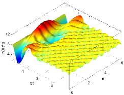
Figure 1: Density as a function of the angle and time for 8 electrons on the ring in a magnetic field of $B=1.41$T.

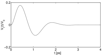
Figure 2: The time-dependent part of the perturbation pulse. The space-dependent part is a simple cosine.

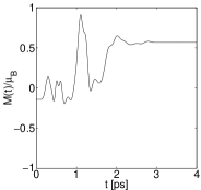
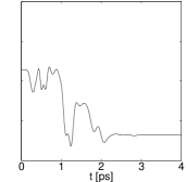
Figure 3: Magnetization as a function of time for 1 electron and $B=1.71$T (left) and $B=4.7$T (right).

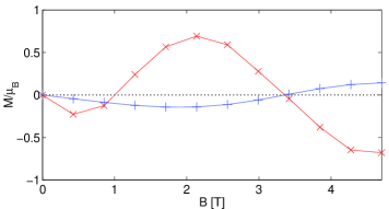
Figure 4: Equilibrium magnetization $M_{0}(0)$ ($+$) and the magnetization $M_{0}(t_{f})$ ($\times$) after the radiation pulse has vanished for one electron. Here $t_{f}$ denotes the final timestep.

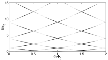
Figure 5: Energy spectrum of the one-dimensional ring as a function of the magnetic flux. The energy is given in units of $\epsilon_{0}=\hbar^{2}/2m^{*}r_{0}^{2}$

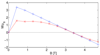
Figure 6: Equilibrium magnetization $M_{0}(0)$ ($+$) and the magnetization $M(t_{f})$ ($\times$) after the radiation pulse has vanished for 8 electrons.

References

- [1] D.K. Ferry and S.M. Goodnick, Transport in Nanostructures (Cambridge University Press, Cambridge, 1997).
- [2] C.S. Tang and C.S. Chu, Phys. Rev. B 53, 4838 (1996).
- [3] C.S. Tang and C.S. Chu, Phys. Rev. B 60, 1830 (1999).
- [4] S. Komlyama, O. Astafiev, V. Antonov, T. Kutsuwa, and H. Hiral, Nature 403, 405 (2000).
- [5] V. Gudmundsson, C.S. Tang, and A. Manolescu, Phys. Rev. B 67, 161301(R) (2003).
- [6] M. Büttiker, Y. Imry, and R. Landauer, Phys. Lett. A 96, 365 (1983).
- [7] R.A. Webb, S. Washburn, C.P. Umbach, and R.B. Laibowitz, Phys. Rev. Lett. 54, 2696 (1985).
- [8] T. Chakraborty and P. Pietiläinen, Phys. Rev. B 50, 8460 (1994).
- [9] V. Gudmundsson and C.S. Tang, eprint: cond-mat/0304571 (to be published).
- [10] W.-C. Tan and J.C. Inkson, Phys. Rev. B 60, 5626 (1999).