Design of a Protein Potential Energy Landscape by Parameter Optimization
Abstract
We propose an automated protocol for designing the energy landscape of a protein energy function by optimizing its parameters. The parameters are optimized so that not only the global minimum energy conformation becomes native-like, but also the conformations distinct from the native structure have higher energies than those close to the native one. We classify low-energy conformations into three groups, super-native, native-like, and non-native ones. The super-native conformations have all backbone dihedral angles fixed to their native values, and only their side-chains are minimized with respect to energy. On the other hand, the native-like and non-native conformations all correspond to the local minima of the energy function. These conformations are ranked according to their root-mean-square deviation (RMSD) of backbone coordinates from the native structure, and a fixed number of conformations with the lowest RMSD values are defined to be native-like conformations, whereas the rest are defined as non-native ones. We define two energy gaps and . The energy gap is the energy difference between the lowest energy of the non-native conformations and the highest energy of the native-like (super-native) ones. The parameters are modified to decrease both and . In addition, the non-native conformations with larger values of RMSD are made to have higher energy relative to those with smaller RMSD values. We successfully apply our protocol to the parameter optimization of the UNRES potential energy, using the training set of betanova, 1fsd, the 36-residue subdomain of chicken villin headpiece (PDB ID 1vii), and the 10-55 residue fragment of staphylococcal protein A (PDB ID 1bdd). The new protocol of the parameter optimization shows better performance than earlier methods where only the difference between the lowest energies of native-like and non-native conformations was adjusted without considering various degrees of native-likeness of the conformations. We also perform jackknife tests on other proteins not included in the training set and obtain promising results. The results suggest that the parameters we obtained using the training set of the four proteins are transferable to other proteins to some extent.
I introduction
The prediction of the three-dimensional structure and the folding pathway of a protein solely from its amino acid sequence is one of the most challenging problems in biophysical chemistry. There are two major approaches to the protein structure prediction, so called knowledge-based methods and energy-based methods. The knowledge-based methods[1, 2, 3, 4], which include comparative modeling and fold recognition, use statistical relationship between sequences and their three-dimensional structures in the Protein Data Bank (PDB), without deep understanding of the interactions governing the protein folding. Therefore, although these methods can be very powerful for predicting the structure of a protein sequence that has a certain degree of similarity to those in PDB, they cannot provide the fundamental understandings of the protein folding mechanism.
On the other hand, the energy-based methods [5, 6, 7, 8, 9, 10, 11], which are also called the physics-based methods, are based on the thermodynamic hypothesis that proteins adopt native structures that minimize their free energies[12]. Understanding the fundamental principles of the protein folding by these methods will lead not only to the successful structure prediction, especially for proteins having no similar sequences in PDB, but also to the clarification of the protein folding mechanism.
However, there have been several major obstacles to the successful application of energy-based methods to the protein folding problem. First, there are inherent inaccuracies in the potential energy functions which describe the energetics of proteins. Second, even if the global minimum-energy conformation is native-like, this does not guarantee that a protein will fold into its native structure in a reasonable time-scale unless the energy landscape is properly designed, as summarized in the Levinthal paradox.
Physics-based potentials are generally parameterized from quantum mechanical calculations and experimental data on model systems[13]. However, such calculations and data do not determine the parameters with perfect accuracy. The residual errors in potential energy functions may have significant effects on simulations of macromolecules such as proteins where the total energy is the sum of a large number of interaction terms. Moreover, these terms are known to cancel each other to a high degree, making their systematic errors even more significant. Thus it is crucial to refine the parameters of a potential energy function before it can be successfully applied to the protein folding problem.
An iterative procedure which systematically refines the parameters of a given potential energy function was recently proposed[13] and successfully applied to the parameter optimization[13, 14, 16, 15] of a UNRES potential energy[17, 18, 19]. The method exploits the high efficiency of the conformational space annealing (CSA) method[20, 21, 22, 23, 24] in finding distinct low energy conformations. For a given set of proteins, whose low-lying local minimum-energy conformations for a given energy function is found by the CSA method, one modifies the parameter set so that native-like conformations of these proteins have lower energies than non-native ones. The method consists of the following steps:
(1) Low-lying local minimum-energy conformations are searched with no constraints, which is called the global CSA search. For many proteins, the conformations resulting from the global CSA are non-native conformations for parameters that are not optimized yet.
(2) Native-like conformations are searched by the local CSA search, where low-lying local minimum-energy conformations are sampled among those whose root-mean-square deviation (RMSD) of the backbone coordinates from the native structure is below a given cutoff value .
(3) The native-like and non-native conformations from the steps (1) and (2) are added to the structural database of each protein.
(4) Among the conformations in the structural database, those with RMSD below a given cutoff value are defined as native-like conformations, whereas the rest are defined as non-native ones. The parameters are optimized in such a way to minimize the energy gaps
| (1) |
for all proteins in the training set, where is the minimum-energy among the energies of the native-like (non-native) conformations in the structural database.
(5) After the parameters are modified in the step (4), the conformations in the structural database are not local minimum-energy conformations any more. Therefore it is necessary to reminimize these conformations using the potential energy with the new parameters.
(6) In general, with the new parameters, there may exist many additional low-lying local minima of the potential energy, which are absent in the structural database. Therefore, it is necessary to go back to the step (1) and perform CSA searches with the new parameters.
These steps are repeated until the performance of the optimized parameters is satisfactory, i.e., the global CSA search finds native-like conformations with reasonably small values of RMSD from their corresponding native structures. Since the size of the structural database of local minimum-energy conformations grows after each iteration, the efficiency of the parameter optimization increases as the algorithm proceeds.
It would be desirable to include many proteins in the training set that represent many structural classes of proteins. The optimization method was successfully applied to the parameter optimization of the UNRES potential for a training set consisting of three proteins of structural classes and [15], without introducing additional multibody terms [11, 14, 25]. However, it was still difficult to optimize the parameters of the UNRES potential for a training set containing proteins.
In this work, we propose a new protocol where the parameters are modified so as to make conformations with larger values of RMSD have higher values of energy relative to those with smaller values of RMSD. This goal is achieved by using the following modified energy
| (2) |
when calculating the energy gaps, where the numerical value of the coefficient 0.3 is an arbitrarily chosen value. The new method is more natural than previous methods[13, 14, 15] where non-native conformations were treated equally regardless of their RMSD values. It also turns out that the new method is much more efficient than the previous ones and allows us now to optimize the parameters for a training set containing a protein. Additional new features are introduced in the current method to overcome several major drawbacks of the previous methods as below.
First, in previous methods[13, 14, 15], arbitrarily chosen values of RMSD cutoffs and were used as the criteria for separating native-like conformations from non-native ones, which were set at each iteration by inspecting the distribution of RMSD values of conformations. This rather arbitrary procedure made it difficult to automate the optimization procedure. Moreover, for some proteins, the value of had to be taken as a large number in order to have a non-zero number of native-like conformations, in which case the local CSA search is not meaningful. This can happen for a protein where the initial parameter set is so bad that there exist no local minimum-energy conformations which are native-like. This problem is solved in the current method by introducing what we call the super-native conformations, whose backbone angles are fixed to the values of the native structure and only side-chain angles are minimized with respect to the energy. In the current method, the local CSA search is defined as the restricted search for the super-native conformations in the space of the side-chain angles. Since the RMSD values for the super-native conformations are zero by definition, an arbitrary cutoff value is no longer necessary. Also, the super-native conformations can be found for any parameter set. Although the super-native conformations are unstable with respect to the energy, minimizing the energy gap between their highest energy and the lowest energy of non-native conformations has an effect of stabilizing their energies. Therefore, due to the reminimization procedure with new optimized parameters, the super-native conformations would furnish low-lying local minima with small RMSD values which accumulate as the iteration proceeds. This makes the current method more efficient than the earlier methods where it was difficult to optimize the parameters unless local minimum-energy conformations with small values of RMSD exist with the initial parameters. In addition to the super-native conformations, we define native-like conformations as the 50 conformations with the lowest RMSD values in the structural database. Although 50 is an arbitrary number, it can be kept as a fixed number, and again the cutoff value is set automatically. As mentioned above, the low lying local minima with small RMSD values can be provided from the reminimization procedure of the super-native conformations. Generally, the RMSD values of these native-like conformations become smaller as the iteration of the parameter optimization continues. Both super-native and native-like conformations are used for calculating the energy gaps.
Second, we introduce the Linear Programming to systematically perform the parameter optimization based on linear approximation. This allows one to optimize the parameters so that an energy gap of a protein is minimized, while imposing the constraints that the other energy gaps, including those of the other proteins, do not increase if they are positive, and do not become positive if they are negative. This is in contrast to the optimization method of earlier works where the protein with the largest energy gap was selected in turn, and the energy gap of that protein was reduced without imposing any constraint to the energy gaps of the other proteins in the set. Since the Linear Programming has an effect of simultaneously decreasing the energy gaps of all the proteins in the training set, it is especially powerful when there are many proteins in the training set.
In this work, we successfully apply this method to the optimization of linear parameters in the UNRES potential energy, for a training set consisting of betanova, 1fsd, the 36-residue subdomain of chicken villin headpiece (PDB ID 1vii), and the 10-55 residue fragment of staphylococcal protein A (PDB ID 1bdd). We obtain the global minimum energy conformations (GMECs) of these proteins with RMSD values of , , , and Å, respectively. The proteins in the training set are (betanova), (1fsd), and (1vii and 1bdd) proteins, which cover representative structural classes of small proteins in the nature. The basic form of the UNRES potential we use, where the only multibody term is the four-body term, is the one that was used for successful prediction of unknown structures of proteins in CASP3[7, 10, 26]. With the optimized parameters, we have performed jackknife tests on various proteins not included in the training set, and we find promising results.
II Methods
A Potential Energy Function
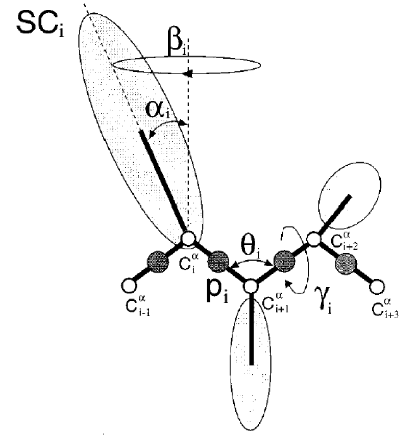
We use the UNRES force field[17, 18, 19], where a polypeptide chain is represented by a sequence of -carbon () atoms linked by virtual bonds with attached united side-chains (SC) and united peptide groups (p) located in the middle between the consecutive ’s (Figure 1). All the virtual bond lengths are fixed: the - distance is taken as Å, and - distances are given for each amino acid type. The energy of the chain is given by
| (4) | |||||
As described in detail in the Appendix of ref.[15], , , , , and can be further decomposed into linear combinations of smaller parts, whose coefficients are refined in this work. Here, represents the mean free energy of the hydrophobic (hydrophilic) interaction between the side-chains of residues and , which is expressed by Lennard-Jones potential, corresponds to the excluded-volume interaction between the side-chain of residue and the peptide group of residue , and the potential accounts for the electrostatic interaction between the peptide groups of residues and . The terms , , and denote the short-range interactions, corresponding to the energies of virtual dihedral angle torsions, virtual angle bending, and side-chain rotamers, respectively. denotes the energy term which forces two cysteine residues to form a disulfide bridge. Finally, the four-body interaction term results from the cumulant expansion of the restricted free energy of the polypeptide chain. The functional form eq (4), as well as the initial parameter set we use, is the one used in the CASP3 exercise[7, 26]. The total number of linear parameters which we adjust is 715 [27].
B Global and Local CSA
In order to check the performance of a potential energy function for a given set of parameters, one has to sample super-native, native-like, and non-native conformations for each protein in the training set. For this purpose we perform two types of conformational search, the local and global CSA searches. In the local CSA, the backbone angles of the conformations are fixed to the values of the native conformations, and only the side-chain energy is minimized with respect to the energy. We call the resulting conformations the super-native. The other conformations are obtained from unrestricted conformational search which we call global CSA. The conformations obtained from the local and global searches are added to the structural database of local minimum-energy conformations for each protein.
C Parameter Refinement Using Linear Programming
The changes of energy gaps are estimated by the linear approximation of the potential energy in terms of parameters. Among the conformations with non-zero RMSD values in the structural database, 50 (an arbitrary number) conformations with the lowest RMSD values are defined as the native-like conformations, while the rest are defined to be the non-native ones. Since a potential can be considered to describe the nature correctly if native-like structures have lower energies than the non-native ones, the parameters are optimized to minimize the energy gaps and ,
| (5) | |||||
| (6) |
for each protein in the training set, where and are the highest energies of the native-like and super-native conformations, respectively, and is the lowest energy of the non-native conformations. The energies are the modified ones that are weighted with the RMSD values of the conformations as in eq (2). Weighting the energy with the RMSD value has the effect of “pushing harder” the high RMSD conformations compared to the ones with lower RMSD values. This idea is somewhat similar to the hierarchical optimization method proposed in ref.[16], where the secondary structure contents were used for the criterion for ranking the nativeness of conformations. In this work we simply use the RMSD values. The RMSD value is easier to calculate and consequently it becomes easier to automate the procedure. The parameter optimization is carried out by minimizing the energy gaps and of each protein in turn, while imposing the constraints that all the other energy gaps, including those from the other proteins, do not increase.
In this work, we adjust only the linear parameters for simplicity, the total number of them being 715 for the UNRES potential. Therefore the energy of a local minimum energy conformation can be written as:
| (7) |
where ’s are the energy components evaluated with the coordinates of a local minimum-energy conformation. Since the positions of the local minima also depend on the parameters, the full parameter dependence of the energy gaps are nonlinear. However, if the parameters are changed by small amounts, the energy with the new parameters can be estimated by the linear approximation:
| (8) |
where the and terms represent the parameters before and after the modification, respectively. The parameter dependence of the position of the local minimum can be neglected in the linear approximation, since the derivative in the conformational space vanishes at local minima[13]. The additional term 0.3 RMSD of eq.(2) vanishes in these expressions due to the same reason. The change of the energy gaps are estimated as:
| (9) | |||||
| (10) | |||||
| (11) |
| (12) | |||||
| (13) | |||||
| (14) |
The magnitude of the parameter change is bounded by a certain fraction of . We use in this study. First, the vector is chosen within the bound to decrease the energy gap of the selected protein as much as possible while imposing the constraints that any positive values among and the energy gaps of the other proteins do not increase and negative values do not become positive. Denoting the energy gaps of the -th protein as and assuming the -th protein is selected for the decrease of the energy gap, this problem can be phrased as follows:
Minimize
| (15) |
with constraints
| (16) |
| (17) |
| (18) |
This is a global optimization problem where the linear parameters are the variables. The object function to minimize and the constraints are all linear in . This type of the optimization problem is called the Linear Programming. It can be solved exactly, and many algorithms have been developed for solving the Linear Programming problem. We use the primal-dual method with supernodal Cholesky factorization [28] in this work, which finds a reasonably accurate answer in a short time.
After minimizing , we solve the same form of linear programming where now are the objective function and the other energy gap changes become constrained. Then we select another protein and repeat this procedure (300 times in this work) of minimizing and in turn.
The current optimization procedure is different from the one used in the earlier works[15] where optimization was performed without using super-native conformations, and energy was not weighted with RMSD values. The earlier procedure and the current one are shown schematically in Figure 2 and Figure 3, respectively, in terms of energy and RMSD.
D Reminimization and New Conformational Search
Since the procedure of the previous section was based on the linear approximation eqs (11) and (14), we now have to evaluate the true energy gaps using the newly obtained parameters. The breakdown of the linear approximation may come from two sources. First, the conformations corresponding to the local minima of the potential for the original set of parameters are no longer necessarily so for the new parameter set. For this reason, we reminimize the energy of these conformations with the new parameters. Since the super-native conformations are not local minimum-energy conformations, even with the original parameters, the reminimization of these conformations with the new parameters would furnish low-lying local minima with small values of RMSD. Second, the local minima obtained using CSA method with the original parameter set may constitute only a small fraction of low-lying local minima. After the change of the parameters, some of the local minima which were not considered due to their relatively high energies, can now have low energies for the new parameter set. It is even possible that entirely distinct low-energy local minima appear. Therefore these new minima are taken into account by performing subsequent CSA searches (See section B.) with the newly obtained parameter set.
E Update of the Structural Database and Iterative Refinement of Parameters
The low-lying local energy minima found in the new conformational searches are added into the energy-reminimized conformations to form a structural database of local energy minima. The conformations in the database are used to obtain the energy gaps, which are used for the new round of parameter refinement. As the procedure of [CSA parameter refinement energy reminimization] is repeated, the number of conformations in the structural database increases[15]. This iterative procedure is continued until sufficiently good native-like conformations are found from the global CSA search.
III Results
A Four Proteins in the Training Set
We apply our protocol to a training set consisting of four proteins. They are the designed protein betanova, 1fsd, 36 residue subdomain of chicken villin headpiece (HP36 or 1vii), and 10-55 fragment of the B-domain of staphylococcal protein A (1bdd), which are 20, 28, 36, 46 residues long, respectively. The protein betanova is a protein, 1fsd is a protein, and the rest are proteins, which represent structural classes of small proteins. The initial parameter set is the one used in CASP3[7, 26].
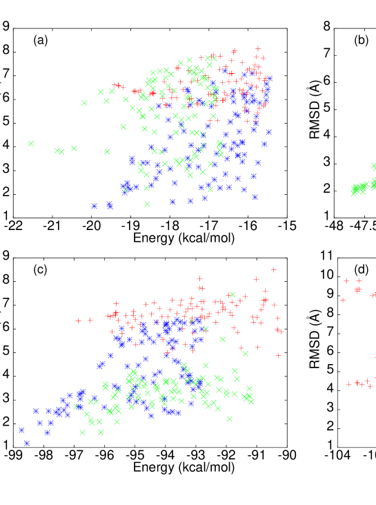
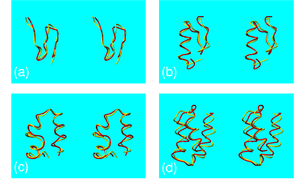
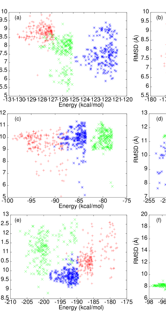
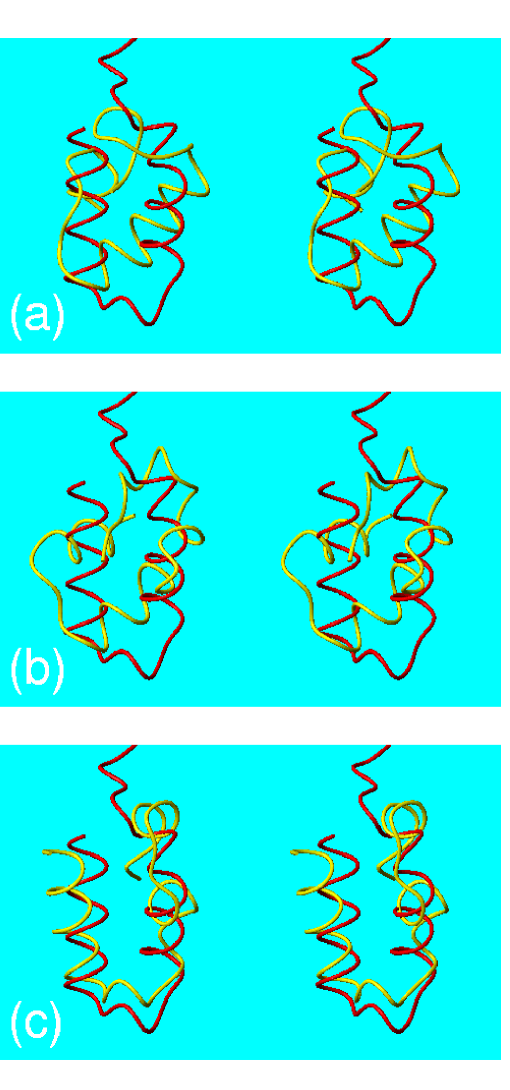
Fifty conformations were sampled in each CSA search, and the global minimum-energy conformations (GMECs) found with the initial parameters have RMSD values of , , and Å, respectively, and the smallest values of RMSD found from the CSA search are , , and Å. After the 28-th iteration of the parameter refinement, the conformations with smaller values of RMSD are found from the global CSA search. The GMECs have RMSD values of , , and Å and the smallest values of RMSD found are , , and Å. The RMSD values become even smaller after the 40-th iteration with RMSDs of GMECs being , , and Å and the smallest values of RMSD being , , and Å. The RMSDs of the GMECs and the lowest RMSDs for these parameters are shown in the table I. The results of the global search with the initial and optimized parameter set for the four proteins are also plotted in different colors in terms of energy and RMSD in Figure 4. The local energy conformations accumulated in the structural databases after the 40-th iteration of the parameter refinement are shown in Figure 5 along with the global CSA search results. The traces of the GMECs of the four proteins found using the parameters obtained after the 40-th iteration of optimization are shown in Figure 6 along with the native conformations.
We also observe a linear slope of in the energy vs. RMSD plot for the low-lying states. It turns out that the energy landscape designed this way assures a good foldability. In fact, the direct Monte Carlo folding simulation with the UNRES potential using the parameters after the 40-th iteration of the refinement, could successfully fold all four proteins into their native states[29].
B Jackknife Tests
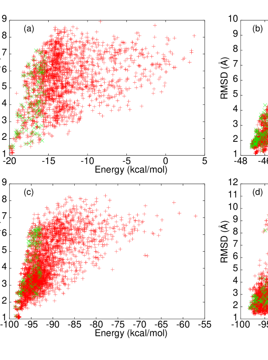
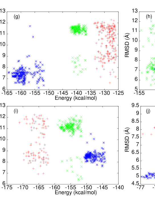
We have performed conformational searches for proteins not contained in the training set, which are usually called jackknife tests. We selected proteins of various structural classes, composed of no more than 60 amino acids residues. We considered proteins from NMR experiments, since the protein structures in the training set are all determined by NMR spectroscopy. We find that the performance of the optimized parameters is reasonably good, and the optimized parameter set provides better performance compared to the results from the initial parameter set. This implies that the optimized parameters are not overfitted to the four proteins in the training set, but are transferable to other proteins to some extent.
We have considered proteins 1bbg, 1ccn, 1hnr, 1kbs, 1neb, 1bba, 1idy, 1prb, 1pru, and 1zdb, with the number of amino-acid residues being 40, 46, 47, 60, 60, 36, 54, 53, 56, and 38, respectively. The protein 1bbg, 1ccn, and 1hnr are proteins, 1kbs and 1neb are proteins, and the rest are proteins. The RMSD values of GMECs and the best structures found with initial and optimized parameter set are shown in Table I. The results are also shown in terms of energy and RMSD in Figures 7. We find that the results for the protein 1zdb is particularly notable. In figure 8, the traces of the GMECs found with initial and optimized parameters are shown together with the native structure. We see that although this protein is not included in the training set, the GMEC becomes more and more similar to the native structure as the parameter optimization procedure is continued. These results suggest that the parameters we obtained from the training set of the four proteins provide better performances than the initial parameter set, and are transferable to other proteins.
IV Discussion
We have proposed a general protocol for the force field parameter optimization and landscape design, and applied it to the UNRES potential. We optimized the 715 linear parameters so that they correctly describe the energetics of four proteins simultaneously. This optimized parameter set yielded GMECs with RMSD values of , , , and Å for betanova, 1fsd, 1vii, and 1bdd, respectively. In the process we designed the energy landscape to have a good foldability[29]. It seems that the current parameter optimization method achieves this goal by constructing the protein folding funnel[30], which is believed to be an essential property of the protein energy functions in nature. It would be interesting to see how many proteins can be energetically well described using a given force field. This should provide a good measure for the efficacy of existing force fields.
In contrast to the earlier protocols[13, 15], where the value of RMSD cutoff values was specified for each protein at each iteration to define native-like conformations, we now defined 50 conformations with the lowest RMSD values in the structural database for each protein as the native-like conformations and used super-native structures, which have zero RMSD values by definition, to furnish candidates for low-lying native-like conformations of small values of RMSD. This enabled us to automate the whole procedure using a shell script. However, there is still some arbitrariness in our protocol, such as choosing 50 native-like conformations, and giving the slope of in eq (2). We also tried the values of and , with similar results as in the case of . We will have to devise a way of choosing the optimal value of the slope. Finally, it should be noted that although we have considered only the UNRES potential for parameter optimization in this work, it is straightforward to apply the same procedure to other potentials such as ECEPP[31], AMBER[32], CHARMM[33] with various solvation terms[34, 35]. All these points are left for the future study.
ACKNOWLEDGMENTS
We thank Ki Hyung Joo and Il-Soo Kim for useful discussions and helps in fulfilling this work. This work was supported by grant No. R01-2003-000-11595-0 (Jooyoung Lee) and No. R01-2003-000-10199-0 (Julian Lee) from the Basic Research Program of the Korea Science & Engineering Foundation. The calculation was carried out on Linux PC cluster of 214 AMD processors at KIAS.
REFERENCES
- [1] Jones, T. A.; Kleywegt, G. J. Proteins Struct. Funct. Genet. Suppl. 1999, 3, 30.
- [2] Murzin, A. G. Proteins Struct. Funct. Genet. Suppl. 1999, 3, 88.
- [3] Tramontano, A.; Leplae R.; Morea V. Proteins Struct. Funct. Genet. Suppl. 2001, 5, 22.
- [4] Sippl, M. J.; Lackner, P.; Domingues, F. S.; Prlić, A.; Malik, R.; Andreeva, A.; Wiederstein, M. Proteins Struct. Funct. Genet. Suppl. 2001, 5, 55.
- [5] Orengo, C. A.; Bray, J. E.; Hubbard, T.; LoConte, L.; Sillitoe, I. Proteins Struct. Funct. Genet. Suppl. 1999, 3, 149.
- [6] Lesk, A. M.; LoConte L.; Hubbard, T. Proteins Struct. Funct. Genet. Suppl. 2001, 5, 98.
- [7] Lee, J.; Liwo, A.; Ripoll, D. R.; Pillardy, J.; Scheraga, H. A. Proteins Struct. Funct. Genet. Suppl. 1999, 3, 204.
- [8] Lee, J.; Liwo, A.; Scheraga, H. A. Proc. Natl. Acad. Sci. U.S.A. 1999, 96, 2025.
- [9] Liwo, A.; Lee, J.; Ripoll, D. R.; Pillardy, J.; Scheraga, H. A. Proc. Natl. Acad. Sci. USA 1999, 96, 5482.
- [10] Lee, J.; Liwo, A.; Ripoll, D. R.; Pillardy, J.; Saunders, J. A.; Gibson; K. D.; Scheraga, H. A. Int. J. Quantum Chem. 2000, 77, 90.
- [11] Pillardy, J.; Czaplewski, C.; Liwo, A.; Lee, J.; Ripoll, D.; Kaźmierkiewicz, R.; Oldziej, S.; Wedemeyer, W. J.; Gibson, K. D.; Arnautova, Y. A.; Saunders, J.; Ye, Y.; Scheraga, H. A. Proc. Natl. Acad. Sci. U.S.A. 2001, 98, 2329.
- [12] Anfinsen, C. B. Science 1973, 181, 223.
- [13] Lee, J.; Ripoll, D. R.; Czaplewski, C.; Pillardy, J.; Wedemeyer, W. J.; Scheraga, H. A. J. Phys. Chem. B 2001, 105, 7291.
- [14] Pillardy, J.; Czaplewski, C.; Liwo, A.; Wedemeyer, W. J.; Lee, J.; Ripoll, D.; Arlukowicz, P.; Oldziej, S.; Arnautova, Y. A.; Scheraga, H. A. J. Phys. Chem. 2001, B, 105, 7299.
- [15] Lee, J.; Park, K.; Lee, J. J. Phys. Chem. B 2002, 106, 11647.
- [16] Liwo, A.; Arlukowicz, P.; Czaplewski, C.; Oldziej, S.; Pillardy, J.; Scheraga, H. A. Proc. Natl. Acad. Sci. U.S.A. 2002, 99, 1937.
- [17] Liwo, A.; Oldziej, S.; Pincus, M. R.; Wawak, R. J.; Rackovsky, S.; Scheraga, H. A. J. Comput. Chem. 1997, 18, 849.
- [18] Liwo, A.; Pincus, M. R.; Wawak, R. J.; Rackovsky, S.; Oldziej, S.; Scheraga, H. A. J. Comput. Chem. 1997, 18, 874.
- [19] Liwo, A.; Kaźmierkiewicz, R.; Czaplewski, C.; Groth, M.; Oldziej, S.; Wawak, R. J.; Rackovsky, S.; Pincus, M. R.; Scheraga, H. A. J. Comput. Chem. 1998, 19, 259.
- [20] Lee, J.; Scheraga, H. A.; Rackovsky. S. J. Comput. Chem. 1997, 18, 1222.
- [21] Lee, J.; Scheraga, H. A.; Rackovsky. S. Biopolymers 1998, 46, 103.
- [22] Lee, J.; Scheraga, H. A. Int. J. Quantum Chem. 1999, 75, 255.
- [23] Lee, J.; Lee, I.H.; L ee, J. Phys. Rev. Lett. 2003, 91, 080201.
- [24] Kim S-Y; Lee S.J.; Lee J. J. Chem. Phys. 2003, in press.
- [25] Liwo, A.; Czaplewski, C.; Pillardy, J.; Wawak, R. J.; Rackovsky, S.; Pincus, M. R.; Scheraga, H. A. J. Chem. Phys. 2001, 115, 2323.
- [26] Third Community Wide Experiment on the Critical Assessment of Techniques for Protein Structure Prediction; Asilomar Conference Center, December 13-17, 1998; http://predictionscenter.llnl.gov/casp3/Casp3.html.
- [27] The number of parameters are larger than 709 used in ref [15] since now we allow different weights to the four-body terms for parallel and anti-parallel strands. Also, whereas the side-chain peptide group interaction and 14 rescaling (See Appendix.) were performed in an asymmetric manner in earlier works, we do it symmetrically.
- [28] Mészáros, C. A. Computers & Mathematics with Applications 1996, 31 49.
- [29] Kim, S.-Y.; Lee, J.; Lee, J., “Folding Mechanism of Small Proteins”, cond-mat/0306517 (available at http://xxx.lanl.gov/cond-mat)
- [30] Onuchic, J. N.; Luthy-Schulten, Z.; Wolynes, P. G. Annu. Rev. Phys. Chem. 1997, 48, 545.
- [31] Némethyi, G.; Gibson, K. D.; Palmer, K. A.; Yoon, C. N.; Paterlini, G.; Zagari, A.; Rumsey, S.; Scheraga, H. A. J. Phys. Chem. 1992, 96, 6472.
- [32] Pearlman, D. A.; Case, D. A.; Caldwell, J. W.; Ross, W. S.; Cheatham III, T. E.; DeBolt, S.; Ferguson, D.; Seibel, G.; Kollman, P. Comp. Phys. Commun. 1995, 91, 1.
- [33] Brooks, B. R.; Bruccoleri, R. E.; Olafson, B. D.; States, D. J.; Swaminathan, S.; Karplus, M. J. Comp. Chem. 1983, 4, 187.
- [34] Ooi, T.; Oobatake, M.; Nemethy, G.; Scheraga, H. A.; Proc. Natl. Acad. Sci. 1987, 84, 3086.
- [35] Wesson, L.; Eisenberg, D. Prot. Sci. 1992, 1, 227.
- [36] Koradi, R.; Billeter, M.; Wuthrich, K. J. Mol. Graphics 1996, 14, 51.
| protein | 0-th | 28-th | 40-th |
|---|---|---|---|
| betanova ( : 20 aa) | 6.6 (5.1) | 4.1 (1.6) | 1.5 (1.5) |
| 1fsd ( : 28 aa) | 5.6 (3.6) | 1.9 (1.7) | 1.7 (1.3) |
| 1vii ( : 36 aa) | 6.3 (4.9) | 2.7 (1.6) | 1.7 (1.2) |
| 1bdd ( : 46 aa) | 9.6 (4.0) | 3.1 (1.6) | 1.9 (1.7) |
| 1bbg ( : 40 aa) | 8.7 (6.3) | 7.9 (5.3) | 7.3 (5.9) |
| 1ccn ( : 46 aa) | 7.7 (6.4) | 9.5 (7.0) | 6.5 (6.0) |
| 1hnr ( : 47 aa) | 9.9 (5.1) | 9.7 (5.9) | 9.2 (5.2) |
| 1kbs ( : 60 aa) | 11.2 (9.5) | 11.3 (10.0) | 10.1 (7.6) |
| 1neb ( : 60 aa) | 10.9 (9.3) | 11.3 (8.8) | 9.6 (9.1) |
| 1bba ( : 36 aa) | 8.9 (8.1) | 8.1 (6.8) | 12.0 (10.7) |
| 1idy ( : 54 aa) | 11.9 (6.6) | 11.6 (7.4) | 7.5 (6.2) |
| 1prb ( : 53 aa) | 10.2 (7.0) | 11.1 (5.4) | 7.1 (5.1) |
| 1pru ( : 56 aa) | 8.4 (7.1) | 11.3 (6.4) | 8.4 (7.6) |
| 1zdb ( : 38 aa) | 7.7 (6.3) | 7.6 (4.9) | 5.0 (4.5) |