SLOW DYNAMICS AND LOCAL QUASI-EQUILIBRIUM. RELAXATION IN SUPERCOOLED COLLOIDAL SYSTEMS

Abstract

We present a Fokker-Planck description of supercooled colloidal systems exhibiting slow relaxation dynamics. By assuming the existence of a local quasi-equilibrium state during the relaxation of the system, we derive a non-Markovian Fokker-Planck equation for the non-stationary conditional probability. A generalized Stokes-Einstein relation containing the temperature of the system at local quasi-equilibrium instead of the temperature of the bath is obtained. Our results explain experiments showing that the diffusion coefficient is not proportional to the inverse of the effective viscosity at frequencies related to the diffusion time scale.

I Introduction

The dynamics of slow relaxation systems exhibits peculiar characteristics which make it essentially different from the dynamics of systems relaxing in much shorter time scales angell -nowak . The aging behaviour of the correlation functions struick6 and the violation of the fluctuation-dissipation theorem kurchan and of the Stokes-Einstein relation bonn6 are among those significant features which have attracted the interest of many researchers in the last few years. Relaxation phenomena in glasses, polymers, colloids and granular matter provide innumerable situations demanding new theoretical developments whose implementation constitutes a challenge for nonequilibrium statistical mechanics theories.

The origin of that peculiar behaviour lies in the fact that during its evolution, the system rests permanently away from equilibrium. This feature would justify why results obtained when the system is close to equilibrium are not necessary valid when that condition is not fulfilled. A simple example illustrating this point is supplied from the slow dynamics of a two-level system. During the transition, the system does not thermally equilibrate with the bath and as a consequence equipartition law is not valid. It was shown in origin6 that coarsening the level of description of the path that the system follows in the configuration space going from diffusion to activation regimes leads to violation of the fluctuation-dissipation theorem. The fast decay of the diffusion modes makes the system always close to equilibrium whereas the activation process occurring at longer time scales does not guarantee validity of the theorem.

In this paper we will present an example illustrating the peculiar dynamics of slow relaxation systems. Using a Fokker-Planck description we derive a generalized Stokes-Einstein relation for supercooled colloidal liquids showing that diffusion coefficient and inverse of viscosity are not proportional to each other at low frequencies, when the system becomes activated. At higher frequencies, the particles undergo diffusion in the solvent and that relation holds.

The paper will be distributed as follows. In Section II, we will briefly review the generalization of the Onsager fluctuation theory to nonequilibrium aging states. Section III will be devoted to the formulation of a mean field theory describing the dynamics of high concentrated suspensions. This theory will be used in Section IV to interpret experimental results supporting the violation of the Stokes-Einstein relation in supercooled colloidal liquids. In the conclusions section we will summarize our main results.

II Slow relaxation dynamics and local quasi-equilibrium

When the relaxation of a system is slow enough, its evolution takes place through a sequence of states characterized by a set of thermodynamical quantities in which the intensive parameters are, in general, different from those of the bath. It is then said that the system is at quasi-equilibrium.

A statistical mechanics description of those systems involves the non-stationary conditional probability density $P(\underline{\alpha}_{0},t_{0}|\underline{\alpha},t)$, with $\underline{\alpha}=(\alpha_{1},...,\alpha_{n})$ representing the state vector of the system, and $\underline{\alpha}_{0}$ the initial state at time $t_{0}$. The local quasi-equilibrium states are characterized by the probability density $P_{qe}(\underline{\alpha},t)$ satisfying

$$\lim_{t\rightarrow\infty}P(\underline{\alpha}_{0},t_{0}|\underline{\alpha},t)=P_{qe}(\underline{\alpha},t).$$ (1)

When relaxation takes place in a short time scale, $P_{qe}(\underline{\alpha},t)$ reduces to the local equilibrium probability density in which the intensive parameters are those of the bath.

The evolution of the conditional probability density is governed by a Fokker-Planck equation. To obtain it, we will first formulate the continuity equation

$$\frac{\partial}{\partial t}P(\underline{\alpha}_{0},t_{0}|\underline{\alpha},t)=-\frac{\partial}{\partial\underline{\alpha}}\cdot\left[P(\underline{\alpha}_{0},t_{0}|\underline{\alpha},t)\underline{v}_{\underline{\alpha}}(\underline{\alpha}_{0},\underline{\alpha};t_{0},t)\right],$$ (2)

in which $P\underline{v}_{\underline{\alpha}}$ represents the phase space probability current with $\underline{v}_{\underline{\alpha}}$ the stream velocity in $\underline{\alpha}$-space. That velocity can be obtained from a mesoscopic version of the nonequilibrium thermodynamics for slow relaxation systems we have proposed Slow6 .

The existence of a local quasi-equilibrium state in $\underline{\alpha}$-space enables one to formulate the Gibbs equation

$$T(t)\delta s_{qe}(t)=\delta e_{qe}(t)-\int\mu_{qe}(t)\delta P(t)d\underline{\alpha},$$ (3)

where $s_{qe}(t)$ is the entropy and $e_{qe}(t)$ the mean internal energy per unit mass at quasi-equilibrium . We will assume that the temperature $T(t)$ of the system at local quasi-equilibrium is only a function of time whereas the chemical potential $\mu_{qe}(t)$ can be a function of $\underline{\alpha}$.

The entropy of the system can be expressed in terms of the probability density by means of the Gibbs entropy postulate kampenSuper in the form

$$s(t)=-\frac{k}{m}\int P(t_{0}|t)\ln\frac{P(t_{0}|t)}{P_{qe}(t)}d\underline{\alpha}+s_{qe}(t),$$ (4)

where $k$ is the Boltzmann constant and $m$ the molecular mass.

The form of the current $P\underline{v}_{\underline{\alpha}}$ can be inferred from the entropy production by relating it, as done in nonequilibrium thermodynamics degroot6 , with the corresponding thermodynamic force. The entropy production is obtained by combining the rate of change of $s_{qe}(t)$ obtained from Eq. (3) with the time derivative of Eq. (4). After using Eq. (2) and integrating by parts assuming that $P(t_{0}|t)\underline{v}_{\underline{\alpha}}(t_{0},t)$ vanishes at the boundary, one may identify the non-equilibrium chemical potential $\mu(t_{0};t)=\mu_{qe}(t)+\frac{kT(t)}{m}\ln\frac{P(t_{0}|t)}{P_{qe}(t)}$ and the corresponding thermodynamic force $\frac{\partial\mu(t)}{\partial\underline{\alpha}}$, which is conjugated to the probability current $P\underline{v}_{\underline{\alpha}}$. Following the scheme of nonequilibrium thermodynamics one simply obtains

$$\underline{v}_{\underline{\alpha}}(t_{0};t)=-\underline{\underline{B}}(t_{0};t)\cdot\left[\underline{X}(\underline{\alpha},t)+\frac{kT(t)}{m}\frac{\partial}{\partial\underline{\alpha}}\ln P(t_{0}|t)\right],$$ (5)

where we have defined the generalized force degroot6

$$\underline{X}(\underline{\alpha},t)\equiv-\frac{\partial}{\partial\underline{\alpha}}\left[\frac{kT(t)}{m}\ln P_{qe}(t)\right].$$ (6)

The time dependent transport coefficients $\underline{\underline{B}}(t_{0};t)$ (related to the Onsager coefficients) incorporate memory effects through its dependence on time Fp-nonmarkovian6 , oliveiraEURO , and the local quasi-equilibrium probability density is given by

$$P_{qe}(t)=P_{e}e^{\frac{m}{k\,T(t)}[\mu_{qe}-e_{qe}]},$$ (7)

where $P_{e}$ is the equilibrium distribution function. Eq. (7) can be obtained by using the statistical definition of the entropy in the Gibbs equation (3), Slow6 . Now, by substituting Eq. (5) into (2) the resulting Fokker-Planck equation is

$$\frac{\partial P(t_{0}|t)}{\partial t}=\frac{\partial}{\partial\underline{\alpha}}\cdot\underline{\underline{B}}(t_{0};t)\cdot\left[\underline{X}(\underline{\alpha},t)P(t_{0}|t)+\frac{kT(t)}{m}\frac{\partial P(t_{0}|t)}{\partial\underline{\alpha}}\right],$$ (8)

Using the Fokker-Planck equation (8), we can calculate the evolution equation for the equal-time correlation function of $\underline{\alpha}$-variables which for sufficiently long times leads to the following expression for the temperature of the system

$$T(t)\equiv\frac{m}{k}\left\langle\underline{X}(t)\cdot\underline{\alpha}(t)\right\rangle_{qe},$$ (9)

with $\left\langle...\right\rangle_{qe}$ denoting average at local quasi-equilibrium. This result reduces to the one corresponding to fast relaxation processes degroot-pp88 in which the average is performed at local equilibrium.

In Ref. Slow6 , we have shown that the temperatures of the system and of the bath $T_{B}(t)$ are related by $T(t)=AT_{B}(t)$, expressing lack of thermal equilibration. Equilibrium is reached when $A=1$ in which case, for linear thermodynamic forces, one recovers the expression for equipartition law. The presence of $T(t)$ in the last term of Eq. (8), gives rise to a modified version of the fluctuation-dissipation theorem.

III Fokker-Planck description of concentrated colloidal suspensions

In this section, we will study diffusion in concentrated colloidal suspensions by means of an effective medium approach elaborated on the grounds of the theory we have introduced in the previous section. We will analyze the motion of a test colloidal particle through the suspension by using the Fokker-Planck equation describing the evolution of the two-time probability density $P(\underline{\alpha}_{0},t_{0}|\underline{\alpha},t)$. In this case, the phase space vector is simply $\underline{\alpha}=(\vec{u},\vec{r})$, where $\vec{u}$ and $\vec{r}$ represent the velocity and position of the test particle.

To derive the Fokker-Planck equation, we will first formulate the Gibbs equation

$$T\rho\delta s=\rho\delta e-\rho^{-1}p\delta\rho-m\int\mu\delta Pd\vec{u},$$ (10)

which incorporates the effects of interactions among particles through the term containing the excess of osmotic pressure $p$. Here $e$ is the internal energy, $m$ the mass of the particle and $\rho=m\int Pd\vec{u}$ the mass density. In this case, the quasi-equilibrium probability density is given by Slow6

$$P_{qe}=e^{\frac{m}{2kT}\left[\mu_{qe}-\frac{1}{2}u^{2}-\rho^{-1}p\right]}.$$ (11)

Here, the interaction of the test particle with the other colloidal particles is represented by means of the term $\rho^{-1}p$ which can be expressed in terms of a virial expansion in $\rho$, whereas $\mu_{qe}$ constitutes the ideal chemical potential. Introducing the fugacity $z=P\,a$, with the activity coefficient given by $a\equiv e^{\frac{m}{kT}\rho^{-1}p}$, Eq. (4) can be expressed as

$$s=-\frac{k_{B}}{\rho}\int P\,\ln\frac{z}{z_{qe}}d\vec{u}+s_{qe},$$ (12)

where $z_{qe}=e^{\frac{m}{kT}[\mu_{qe}-\frac{1}{2}u^{2}]}$ is the fugacity at quasi-equilibrium. Notice that in the limit of infinite dilution $\rho^{-1}p\cong 0$, thus implying $a=1$, which corresponds to the ideal case.

The existence of interactions among the test and the other colloidal particles, gives rise to a force term in the continuity equation for $P$. In particular, according to Eq. (11), the force entering into this term is given by $-\nabla(\rho^{-1}p)$ (see for example Ref. mayorgas ). Now, by taking into account the definition of the activity coefficient $a$, the continuity equation for $P$ becomes

$$\frac{\partial P}{\partial t}+\nabla\cdot P\vec{u}-\nabla\left[\frac{kT(t)}{m}\ln a\right]\cdot\frac{\partial P}{\partial\vec{u}}=-\frac{\partial}{\partial\vec{u}}\cdot P\vec{v}_{\vec{u}},$$ (13)

where $P\vec{v}_{\vec{u}}$ is the probability current, with $\vec{v}_{\vec{u}}$ the stream velocity in $\vec{u}$-space.

In accordance with the general formalism of nonequilibrium thermodynamics, the expression of the probability current $P\vec{v}_{\vec{u}}$ can be obtained from the entropy production which only contains dissipative terms and is simply given by

$$\sigma=-\frac{m}{T}\int P\vec{v}_{\vec{u}}\cdot\frac{\partial\mu}{\partial\vec{u}}d\vec{u}.$$ (14)

Eq. (14) has been obtained by taking the time derivative of Eq. (12), using Eqs. (13), (11) and (10), and the balance equation for the energy $e(t)$, neglecting viscous dissipation degroot6 . In order to obtain Eq. (14), we have also identified the nonequilibrium chemical potential

$$\mu(t_{0};t)=\mu_{qe}(t)+\frac{kT(t)}{m}\ln\frac{z(t_{0};t)}{z_{qe}(t)}.$$ (15)

By taking into account the definition (6), the resulting generalized Fokker-Planck equation for the two-time probability density is

$$\frac{\partial P}{\partial t}+\nabla\cdot\vec{u}P-\nabla\left[\frac{kT(t)}{m}\ln a\right]\cdot\frac{\partial P}{\partial\vec{u}}=\frac{\partial}{\partial\vec{u}}\cdot\beta(t)\left[\vec{u}P+\frac{kT}{m}\frac{\partial P}{\partial\vec{u}}\right],$$ (16)

where $\beta$ characterizes the dissipation of the kinetic energy of the test particle. This coefficient is, in general, function of time, position and density; its dependence on time is a consequence of the non-Markovian nature of the stochastic process Fp-nonmarkovian6 , oliveiraEURO , tokuyama .

From Eq. (16), we will now derive the evolution equation for the velocity field by taking the time derivative of the momentum $\rho\vec{v}=m\int\vec{u}Pd\vec{u}$ and using Eq. (16). After integrating by parts one obtains

$$\rho\frac{d\vec{v}}{dt}=-\beta\rho\vec{v}-\frac{kT(t)}{m}\left[1+\frac{\partial\ln a}{\partial\ln\rho}\right]\nabla\rho,$$ (17)

where we have used the fact that, in the absence of an externally imposed flow, the second moment $\!\!\,\,\vec{\vec{\mathrm{P}}}\!\!\,\,=m\int(\vec{u}-\vec{v})(\vec{u}-\vec{v})Pd\vec{u}$ can be approximated by $\!\!\,\,\vec{\vec{\mathrm{P}}}\!\!\,\,=\frac{kT}{m}\rho\vec{\vec{1}}$, nosotrosPRE6 .

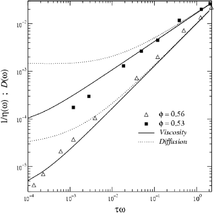
Figure 1: Comparison between the viscosity and diffusion coefficients for two values of the volume fraction. Triangles and squares represent viscosity data from Ref. bonn6 . The gap between viscosity and diffusion at short frequencies is proportional to the scaling factor $A$ of the temperature. At larger frequencies $A\rightarrow 1$.

At times such that $t\gg\beta^{-1}$, the particle enters the diffusion regime in which one may neglect the time derivative in Eq. (17), obtaining then the constitutive relation for the mass diffusion current $\rho\vec{v}$ which substituted into the mass continuity equation $\frac{\partial\rho}{\partial t}=-\nabla\cdot(\rho\vec{v})$, yields the Smoluchowski equation

$$\frac{\partial\rho}{\partial t}=\nabla\cdot\left(D\cdot\nabla\rho\right).$$ (18)

From Eq. (17) we may identify the diffusion coefficient

$$D=\frac{kT(t)}{m\beta}\left[1+\frac{\partial\ln a}{\partial\ln\rho}\right].$$ (19)

The form of Eq. (19) coincides with the expression given in Ref. degroot6 . Notice, however, that it contains the temperature of the system at quasi-equilibrium instead of the temperature of the bath.

III.1 The generalized Stokes-Einstein relation in supercooled colloidal systems

It has been shown in bonn6 that in supercooled colloidal liquids at short frequencies the Stokes-Einstein relation is not fulfilled. Measurements of the viscosity and the diffusion coefficients obtained in Refs. mortensen6 , mason6 , indicate the existence of a frequency domain in which those quantities are not proportional (see figure 1). It is our purpose to offer here an explanation for those experimental results.

In mortensen6 it was shown that the colloidal system can be assumed isotropic and homogeneous at the considered volume fractions, ranging from the freezing to the glass transition values $\phi_{g}$. Consequently, the transport coefficients can be assumed to be independent of the wave vector $\vec{k}$. We will first introduce the effective viscosity

$$\eta(\omega)=\frac{kT}{6\pi R}D^{-1},$$ (20)

where $R$ is the radius of the particle.

The dependence of the viscosity on the frequency can be inferred through the expression of the penetration length $\lambda$ of the diffusive modes. In the dilute case, $\lambda$ is given through $\lambda^{-1}=\frac{1}{R}\left(\tau\omega\right)^{\frac{1}{2}}$, with $\tau=\frac{R^{2}}{6D_{0}}$ the characteristic diffusion time boon-yip and $D_{0}=\frac{kT_{B}}{6\pi R\eta_{0}}$ the diffusivity in the pure solvent, with $\eta_{0}$ its viscosity. At higher concentrations, it can be assumed to be

$$\lambda^{-1}\equiv\frac{1}{\Gamma R}\left(\tau\omega\right)^{\gamma},$$ (21)

where the exponent $\gamma$ and the scaling function $\Gamma$ may, in general, depend on the volume fraction. The quantity $\Gamma R$ can be interpreted as an effective radius.

The penetration length gives an estimation for the average size of a cage formed by the surrounding particles cohen6 . At high frequencies, the test particle performs a free Brownian motion inside the cage and the viscosity is that of the pure solvent. At short frequencies, collisions of the test particle with the other particles modify the viscosity. Thus, we will assume the following expression for the effective viscosity

$$\eta(\omega)=\eta_{0}\left(1+R\lambda^{-1}\right),$$ (22)

valid up to first order in $R\lambda^{-1}$ reflecting the fact that cage diffusion is important when $R\sim\lambda$, cohen-cage .

By taking into account the general relation between system and bath temperatures obtained from our formalism, $T=AT_{B}$, Slow6 , Eq. (20) can be written as

$$D\eta=\frac{kT_{B}}{6\pi R}A,$$ (23)

which constitutes a generalization of the Stokes-Einstein relation to systems exhibiting slow relaxation dynamics.

From Eq. (9) and from its definition, the quantity $A$ is essentially proportional to the velocity moments of the particle. In particular, when $\underline{X}(t)$ is a linear function, $A$ is proportional to the velocity correlation function. It is then plausible to assume the following expansion ngai , tokuyamaslow

$$A\cong\left[1+b\left(\tau\omega\right)^{\epsilon}\right],$$ (24)

where $b$ and the exponent $\epsilon$ may, in general, be functions of the volume fraction $\phi$. Comparison of Eq. (24) with the corresponding relation obtained in bonn6 by fitting the experimental data yields $\ln b\cong\epsilon\left(40\frac{\phi}{\phi_{g}}-37\right)+2.659$, and $\epsilon=-0.77$.

To contrast the theoretical expression of the effective viscosity (22) with the experimental results reported in bonn6 , we will take the logarithm of Eq. (22) and expand the result in terms of the variable $\log\tau\omega$, around $\tau\omega=1$. Up to first order we obtain

$$\log\eta\cong\log\left[\eta_{0}\left(1+\frac{1}{\Gamma}\right)\right]+\frac{\gamma}{1+\Gamma}\log\tau\omega.$$ (25)

A direct comparison of Eq. (25) with the fitting of experimental data given by the expression $\log\eta\cong c_{0}+s(\phi)\log\tau\omega$, with $s(\phi)\approx 6.39-13\phi$ and $c_{0}$ a constant, gives the dependence of $\gamma$ and $\Gamma$ on the volume fraction.

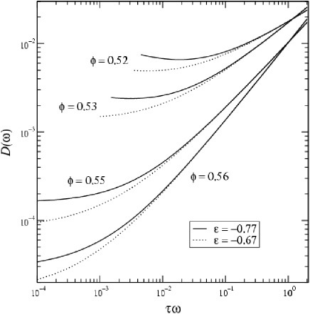
Figure 2: Diffusion coefficient as a function of the frequency for different values of the volume fraction. Solid lines were obtained by fitting the exponent $\epsilon=-0.77$, in accordance with Ref. bonn6 . Dotted lines were obtained by taking $\epsilon=-0.67$.

The expression of the diffusion coefficient at the frequencies we are considering can now be derived by using Eq. (23). In figure 2, we represent the diffusion coefficient given through Eq. (23) as a function of the reduced frequency. At higher concentrations ($\phi=0.56,\,0.55$), a closer agreement with the experimental values of $D$ given in bonn6 has been obtained with $\epsilon=-0.77$ (solid lines). At lower concentrations ($\phi=0.53,\,0.52$), a closer agreement with experiments has been obtained with $\epsilon=-0.67$ (dotted lines). This dependence of the fitting on the value of the exponent $\epsilon$ suggests that it is also a function of the volume fraction.

IV Conclusions

In this paper, we have proposed a general formalism to analyze the dynamics of systems which relax in long time scales of the order of the observation time or even longer. The fact that the system always evolves through transient states never reaching equilibration with the bath is the origin of a peculiar behaviour different from that of systems whose propagating modes relax rapidly ending up in a quiescent state. The dynamics is non-Markovian and the correlation functions exhibit aging effects.

We have formulated a generalization of Onsager’s theory to nonequilibrium aging states to derive a Fokker-Planck equation which captures the main characteristics of the dynamics such as non-stationarity through the two-time probability density, non-Markovianity through the time-dependence of the transport coefficients and lack of thermal equilibration between system and bath. This equation is the main result of our analysis from which the behaviour of the correlation functions follows.

We have applied the theory to study the relaxation in supercooled colloidal liquids for which violation of the Stokes-Einstein relation at low frequencies has recently been found experimentally. The relation between diffusion coefficient and viscosity we have obtained explains those experiments. The key ingredients in this interpretation are the existence of a quasi-equilibrium state with a temperature different from that of the bath which is proportional to the velocity moments and the fact that the viscosity depends on the penetration length of the diffusion modes resulting from the underlying activated process taking place at sufficiently long times.

The formalism proposed thus offers an interesting theoretical framework for the study of glassy behaviour in colloidal liquids.

V Acknowledgments

We want to acknowledge Dr. D. Reguera for valious comments. I.S.H. acknowledges UNAM-DGAPA for economic support. This work was partially supported by DGICYT of the Spanish Government under Grant No. PB2002-01267.

VI Acknowledgments

References

- (1) M. D. Ediger, C. A. Angell and S. R. Nagel, J. Phys. Chem. 100, 13200 (1996).
- (2) P. G. Debenedetti and F. H. Stillinger, Nature, 410, 259 (2001).
- (3) T. S. Grigera and N. E. Israeloff, Phys. Rev. Lett. 83, 5038 (1999).
- (4) F. Sciortino, Nature materials, 1, 145 (2002).
- (5) L. Bellon, S. Ciliberto and C. Laroche, Europhys. Lett. 53, 511 (2001).
- (6) E. R. Nowak, et al, Phys. Rev. E 57, 1971 (1998).
- (7) L.C.E. Struick, Physical aging in amorphous polymers and other materials, Elsevier (1978).
- (8) L. Cugliandolo, J. Kurchan and L. Peliti, Phys. Rev. E 55, 3898 (1997).
- (9) D. Bonn and W. K. Kegel, J. Chem. Phys. 118, 2005 (2003).
- (10) A. Pérez-Madrid, D. Reguera and J. M. Rubí, Physica A, in press. cond-mat/0210089.
- (11) I. Santamaría-Holek, A. Pérez-Madrid and J. M. Rubí, cond-mat/0305605.
- (12) S. R. de Groot and P. Mazur, Non-equilibrium thermodynamics (Dover, New York, 1984).
- (13) N. G. van Kampen, Stochastic processes in physics and chemistry (North-Holland, Amsterdam, 1981).
- (14) I. Santamaría-Holek and J. M. Rubí, Physica A 326, 384 (2003).
- (15) I. V. L. Costa, R. Morgado, M. V. B. T. Lima and F. A. Oliveira, Europhys. Lett. 63, 173 (2003).
- (16) See Ref. degroot6 , pp. 88.
- (17) J. M. Rubí and P. Mazur, Physica A 250, 253 (1998)., M. Mayorga, L. Romero-Salazar and J. M. Rubí, Physica A 307, 297 (2002).
- (18) I . Santamaría-Holek, D. Reguera and J. M. Rubí, Phys. Rev. E 63, 051106 (2001).
- (19) K.G. Wang and M. Tokuyama, Physica A 265, 341 (1999).
- (20) W. van Megen, T. E. Mortensen, S. R. Williams and J. Muller, Phys. Rev. E 58, 6073 (1998).
- (21) T. G. Mason and D. A. Weitz, Phys. Rev. Lett. 75, 2770 (1995).
- (22) J. P. Boon and S. Yip, Molecular hydrodynamics (Dover, New York, 1991).
- (23) R. Verberg, I. M. de Schepper and E. G. D. Cohen, Phys. Rev. E 55, 3143 (1997).
- (24) R. Verberg, I. M. de Schepper and E. G. D. Cohen, Phys. Rev. E 61, 2967 (2000).
- (25) C. A. Angell, et al, J. Appl. Phys. 88, 3113 (2000).
- (26) M. Tokuyama, Phys. Rev. E 62, R5915 (2000).