Vertex Intrinsic Fitness: How to Produce Arbitrary Scale-Free Networks

Abstract

We study a recent model of random networks based on the presence of an intrinsic character of the vertices called fitness. The vertices fitnesses are drawn from a given probability distribution density. The edges between pair of vertices are drawn according to a linking probability function depending on the fitnesses of the two vertices involved. We study here different choices for the probability distribution densities and the linking functions. We find that, irrespective of the particular choices, the generation of scale-free networks is straightforward. We then derive the general conditions under which scale-free behavior appears. This model could then represent a possible explanation for the ubiquity and robustness of such structures.

In the last few years, much attention has focused on the study of complex networks. A network is a mathematical object consisting of a collection of vertices (nodes) connected by edges (links)Bollobas01 ; DM03book . Networks arise in many areas of science: biology KKKR02 ; bio ; bio2 , social sciences ASBS00 ; social1 ; social2 , Internet int1 ; int2 ; int3 , WWWAH00 , etc., where vertices and links can be for example, proteins and their mutual interaction, individuals and sexual relationship Liljeros01 , computers and cable connections. Very interestingly the same non trivial statistical properties appear ubiquitously in all the above situations. A more traditional view, indeed, is represented by the binomial model inspired to the random graph model of Erdős-Rényi ER61 . Here, each vertex has the same probability to connect to any other, resulting in a network whose degree, i.e. number of edges per vertex, has a binomial distribution. This is not the case of the above real data, where instead, the structure is self similar resulting in a scale-free (SF) probability distribution for the degree. More specifically, the degree $k$ of the vertices, i.e. the number of links entering them, is distributed according to a power law $P(k)\propto k^{\alpha}$ with usually $-3<\alpha<-2$.

In order to explain the occurrence of SF networks the ingredients of growth preferential attachment have been introduced bara . The network increases the number of vertices with time, the newcomers tend to be connected with old vertices with large degree. Nevertheless, in some cases, we have the same SF properties without either growth of the system or preferential attachment mechanism. As an example, the finite set of protein interactions in a cell forms a self-similar network. This is done without growth of the system size and ignoring their reciprocal degree. Possibly, some external influence on intrinsic properties like chemical affinity is instead driving the phenomenon.

To take into account this new mechanism, the varying fitness model has been introduced by Caldarelli et al. gcalda . In this model, considering e.g. only undirected graphs, one extracts a real non-negative variable $x$ (the hidden variable) for each vertex of the graph from a probability distribution density $\rho(x)$. This variable $x$ is the fitness of the vertex. Links between vertices are successively formed with a probability function $f(x,y)$, a symmetric function of its arguments.

A static simplified form of the vertex hidden variable model has been considered for only one particular case by Goh et al. goh01 . Bianconi et al. BB01b introduced a fitness mechanism coupled to the preferential attachment. In the paper of Caldarelli et al. gcalda , the onset of SF behavior is instead directly related only to the fitness presence of any kind. This behavior is also checked for different fitness probability distribution densities. Following Ref. gcalda , we present here an exhaustive study on the conditions needed in order to produce a SF network.

The aim of this work is to provide some ingredients to generate SF networks with the vertex hidden variable model and to provide the analytic expressions for the functions $\rho(x)$ and $f(x,y)$ that define SF networks in three special cases.

The fitness model can be easily generalized in order to have more than one fitness variable per vertex PScondmat . In the following, we consider a single real variable $x$ per vertex, with $x\geq 0$. As a probability distribution density function, $\rho$ satisfies $\{\rho(x)\geq 0|\int_{0}^{\infty}\rho(z)dz=1\}$, while the linking probability $0\leq f(x,y)\leq 1$. We define the primitive function of $\rho(x)$, the probability distribution $R(x)=\int_{0}^{x}\rho(z)dz$. Indicating the number of vertices in the graph with $N$, one has the vertex degree

$$k(x)=N\int_{0}^{\infty}\!\!\!f(x,z)\rho(z)dz.$$ (1)

Other quantities of interest are the average nearest neighbor connectivity (vertex degree correlation),

$$K_{\mathrm{nn}}(x)=\frac{N}{k(x)}\int_{0}^{\infty}\!\!\!f(x,z)k(z)\rho(z)dz,$$ (2)

expressing the average degree of vertices that are nearest neighbors of vertices with fitness $x$, and the clustering coefficient (vertex transitivity),

$$C(x)=N^{2}\frac{\int_{0}^{\infty}\!\!\!\int_{0}^{\infty}\!\!\!f(x,y)f(y,z)f(z,x)\rho(y)\rho(z)dydz}{k(x)^{2}},$$ (3)

that counts the fraction of nearest neighbors of vertices with fitness $x$ that are also nearest neighbors each other. Eqs. (1), (2), (3) are valid asymptotically when $N$ approaches infinity. Eqs. (2), (3) were first derived in Ref. BP03 , and expressed in a different form.
If $k(x)$ is an invertible and increasing function of $x$ then the probability distribution $P(k)$ is given by

$$P(k)=\rho(x(k))\cdot x^{\prime}(k)$$ (4)

or, as a function of $x$,

$$P(k(x))=\frac{\rho(x)}{k^{\prime}(x)}.$$ (5)

Since the degree probability is power-law distributed in most of the physical situations, we impose in Eq. (5) $P(k)=ck^{\alpha}$ with $\alpha\in\mathbb{R}$. The constant $c$ is fixed by the the normalization condition $\int_{k_{0}}^{N}P(k)dk=1$:

$$c=\left\{\begin{array}[]{ll}\frac{\alpha+1}{N^{\alpha+1}-k_{0}^{\alpha+1}}&\text{if }\alpha\neq-1\\ \left(\log\frac{N}{k_{0}}\right)^{-1}&\text{if }\alpha=-1\\ \end{array}\right.$$ (6)

with $\displaystyle k_{0}=\lim_{x\rightarrow+0}k(x)$. Note that $k_{0}=\beta N$ for some $0<\beta<1$, and $c\propto N^{-(\alpha+1)}$. Eq. (5) becomes:

$$ck^{\prime}(x)(k(x))^{\alpha}=\rho(x).$$ (7)

By integrating Eq. (7) from $0$ to $x$ we get the following non linear integral equation:

$$k(x)=\left\{\begin{array}[]{ll}\Bigl{(}k_{0}^{\alpha+1}+\frac{\alpha+1}{c}R(x)\Bigr{)}^{\frac{1}{\alpha+1}}&\mathrm{if}\ \alpha\neq-1\\ k_{0}e^{R(x)/c}&\mathrm{if}\ \alpha=-1\\ \end{array}\right.$$ (8)

with $k(x)$ given by Eq. (1).

By multiplying both sides of Eq. (8) by $\rho(x)$ and integrating from $0$ to $\infty$ we get an analytic expression for the average vertex degree $\langle k\rangle$. This expression can be used to express $k_{0}$ as a function of $\langle k\rangle$, so that the final expressions do depend on the physical quantity $\langle k\rangle$ only. For this purpose, the integral on the rhs is simply solved using the relation $\rho(x)dx=dR(x)$.

In the following we show an application of the model in three special cases of interest, comparing the analytic results with numerical simulations. It has to be noticed that once fixed $N$, in order to compute the quantities $P(k)$, $K_{\mathrm{nn}}(k)$, $C(k)$, from ensemble statistics, we need to perform two different average procedures. Firstly, we should extract a $\{x_{i}\}_{i=1\ldots N}$ configuration with the distribution density $\rho(x)$ and keep it fixed, while creating ensemble elements using the linking probability $f(x,y)$ and averaging at the end. Secondly, we should repeat the above procedure a sufficient number of times. We assume that for large enough $N$ and ensemble elements, the procedure of first averaging with respect to the $f$ can be skipped.
Here we focus on two different problems: firstly, what we call direct problem, one assigns a distribution density function $\rho(x)$ and tries to find the linking probability function $f(x,y)$; secondly, what we call inverse problem, one assigns the linking probability function and tries to determine the fitness probability distribution density $\rho(x)$. The inverse problem is by far more complex and interesting than the direct one. For instance, in the case of protein SF network by assuming a reasonable linking function, we can retrieve the probability density distribution of fitness (e.g. some basic property of the macro-molecules).

We start with the special case of $f(x,y)=g(x)h(y)$ where both the direct and inverse problems can be analytically solved. Because of the symmetry of $f(x,y)$ with respect to its arguments one has $g(x)\equiv h(x)$, so that $f(x,y)=g(x)g(y)$. Eq. (1) becomes:

$$k(x)=Ng(x)\int_{0}^{\infty}\!\!\!g(z)\rho(z)dz$$ (9)

that substituted into Eq. (8) gives equations in $g$ and $\rho$. If one fixes a given function $\rho(x)$, the equations in $g(x)$ can be easily solved. Take for instance the second equation corresponding to $\alpha=-1$. One gets:

$$Ng(x)\langle g\rangle=k_{0}e^{R(x)/c},\quad\langle g\rangle=\int_{0}^{\infty}\!\!\!g(z)\rho(z)dz.$$

By multiplying left and right hand side by $\rho(x)$ and integrating from $0$ to $\infty$, considering that $\rho(x)dx=dR(x)$, we get:

$$\langle g\rangle=\sqrt{k_{0}c(e^{1/c}-1)/N}.$$

Finally, the solution reads:

$$g(x)=\sqrt{\frac{k_{0}}{Nc(e^{1/c}-1)}}\,e^{R(x)/c}.$$ (10)

This procedure is applicable for any value of $\alpha$. Eq. (10) generates random networks with degree probability distribution $P(k)\propto 1/k$.
In order to test the result we take the choice reported in the caption of Fig. 1.

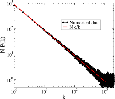
Figure 1: Vertex degree distribution generated by $f(x,y)=g(x)g(y)$, $\alpha=-1$, $\rho(x)=e^{-x}$, $k_{0}=0.1$, $N=10^{4}$. The value of $c$ is calculated from Eq. (6) and the function $g(x)$ from Eq. (10). The number of ensemble elements was $20$.

We conclude that for any given $\rho(x)$ there exists a function $g(x)$ such that the network generated by $\rho(x)$ and $f(x,y)=g(x)g(y)$ is scale free with arbitrary real exponent.

In this case both the average nearest neighbors connectivity and clustering coefficient are constant BP03 . Respectively:

$$K_{\mathrm{nn}}=N\langle g^{2}\rangle,\quad C=\frac{\langle g^{2}\rangle^{2}}{\langle g\rangle^{2}},$$ (11)

as it can be derived from Eq. (2) and Eq. (3).

The inverse problem for $f(x,y)=g(x)g(y)$ is solved by substituting Eq. (9) into Eq. (7):

$$\rho(x)=cg^{\prime}(x)g(x)^{\alpha}(N\langle g\rangle)^{\alpha+1}.$$

Let us remark that the assumptions on $k(x)$ forces $g(x)$ to be non-decreasing with $g(\infty)>g(0)>0$.

In the case $\alpha\neq-1$, the normalization condition $R(\infty)=1$ results in

$$\rho(x)=\frac{\alpha+1}{g(\infty)^{\alpha+1}-g(0)^{\alpha+1}}g^{\prime}(x)g(x)^{\alpha}.$$ (12)

By multiplying both sides of the previous equation by $g(x)$ and integrating from $0$ to $\infty$, one gets an expression for $\langle g\rangle$ that does not explicitly contain the function $\rho(x)$. This expression can be used to get the allowed value of the constant $c$:

$$c=\frac{1}{N^{\alpha+1}}\left[\frac{g_{\infty}^{\alpha+1}-g_{0}^{\alpha+1}}{{\alpha+1}}\right]^{\alpha}\left[\frac{{\alpha+2}}{g_{\infty}^{\alpha+2}-g_{0}^{\alpha+2}}\right]^{\alpha+1}$$

if $\alpha\neq-2$, with $g_{\infty}=g(\infty)$ and $g_{0}=g(0)$. The particular cases $\alpha=\{-1,-2\}$ can be similarly treated.

The case $f(x,y)=f(x-y)$ is more complicated. In this case both the nearest neighbor connectivity and clustering coefficient depend on the fitness $x$ and conversely on the degree $k$. We managed to solve this case in the particular case of an exponentially distributed fitness. We indicate with $F(x)$ the rhs of Eq. (8). Thus Eq. (8) becomes:

$$\int_{0}^{\infty}\!\!\!f(x-u)\rho(u)dx=F(x)/N.$$

By changing the integration variable into $z=x-u$ we get:

$$\int_{-\infty}^{x}\!\!\!\rho(x-z)f(z)dz=F(x)/N$$

that in the special case $\rho(x)=e^{-x}$ becomes:

$$\int_{-\infty}^{x}\!\!\!e^{z}f(z)dz=e^{x}F(x)/N.$$

By differentiating with respect to the variable $x$ we finally obtain:

$$f(x,y)=\frac{F(x-y)+F^{\prime}(x-y)}{N}.$$ (13)

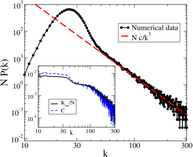
Figure 2: Degree distribution in the case $f(x,y)=f(x-y)$, $\alpha=-3$, $\rho(x)=e^{-x}$, $k_{0}=10$, $N=10^{4}$, $f(u)=F(u)+F^{\prime}(u)$ with $F(x)$ given by the lhs of Eq. (8) averaged $40$ times. The value of $c$ is calculated from Eq. (6). The inset shows the vertex degree correlation and transitivity as functions of the vertex degree.

In order to test the result we take the function and parameter choice of Fig. 2 caption.

The case $f(x,y)=f(x+y)$ is analogous.

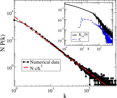
Figure 3: Degree distribution in the case $f(x,y)=f(x+y)$ and $\alpha=-2$, $\rho(x)=e^{-x}$, $k_{0}=0.5$, $N=10^{4}$, $f(v)$ from Eq. (15), averaged $20$ times. The value of $c$ is calculated from Eq. (6). The inset shows the vertex degree correlation and transitivity as functions of the vertex degree.

Again, we consider the special case $\rho(x)=e^{-x}$, getting now:

$$f(x,y)=\frac{F(x+y)-F^{\prime}(x+y)}{N}.$$ (14)

The solution of Eq. (8) for $\alpha=-2$ obtained via Eq. (14) reads, recalling that $k_{0}=\beta N$ and using Eq. (6),

$$f(x,y)=\frac{1}{[1-(\beta^{-1}-1)e^{-(x+y)}]^{2}}.$$ (15)

Through Eq. (15) we clarify the assumption made in the original paper by Caldarelli et al. gcalda , where $f(x,y)=\Theta(x+y-z)$ with $z=z(N)$. Note that now with the latter choice of $f(x,y)$ one gets $P(k)=Ne^{-z}k^{-2}$ that forces $z$ to depend upon $N$ in order to get the correct normalization. The functional form of the $z(N)$ was numerically guessed by Ref. millozzi . To test the result we take the parameters reported in the caption of Fig. 3.

In these last two cases, both the nearest neighbor connectivity and clustering coefficient show non trivial $k$ dependence.

In conclusion we present a general procedure to reproduce real SF networks with arbitrary vertex degree distribution densities. More specifically, we found that, given a fitness distribution density $\rho(x)$, it is always possible to find a symmetric linking probability function $f(x,y)$ such that the resulting random network is scale-free with a given real exponent. We give the recipe to find these linking functions, in three cases of interest. In order to allow the generation of networks even closer to the real data, it would be desirable to have control not only on the vertex degree distribution, but also on the vertex transitivity and vertex degree correlation, by solving simultaneously Eqs. (2), (3), (5). As a first step, the compatibility of these three equations should be addressed, once the functions $P(k)$, $K_{\mathrm{nn}}(k)$, $C(k)$ are given. The solution of this problem is certainly very hard and is left open for the future. The relative ease with which we obtain SF structures seems to be the key ingredient in order to explain the ubiquitous presence and robustness of the real data.

We acknowledge R. Pastor-Satorras, P. De Los Rios, D. Garlaschelli, F. Squartini, S. Millozzi, S. Leonardi for useful discussions and support from EU FET Open Project IST-2001-33555 COSIN (www.cosin.org). VDPS and GC thank IMFM PAIS PA_G02_4 for support.

References

- (1) B. Bollobás, Random Graphs, Academic Press, New York, 2nd ed. (2001).
- (2) S.N. Dorogovtsev and J.F.F. Mendes, Evolution of networks, Oxford University Press, Oxford, (2003).
- (3) J. Kim, P.L. Krapivsky, B. Kahng, and S. Redner, Phys. Rev. E 66, 055101 (2002).
- (4) H. Jeong, S.P. Mason, A.-L. Barabási, and Z.N. Oltvai, Nature 411, 41 (2001).
- (5) D. Garlaschelli, G. Caldarelli and L. Pietronero, Nature, 423, 165 (2003)
- (6) L.A.N. Amaral, A. Scala, M. Barthélémy, and H.E. Stanley, PNAS 97, 11149 (2000).
- (7) M.E.J. Newman, Proc. Natl. Aca. Sci. 98, 404 (2001).
- (8) M.E.J. Newman, Phys. Rev. E 67, 026126 (2003)
- (9) G. Caldarelli, R. Marchetti, and L. Pietronero, Europhys. Lett. 52, 386 (2000).
- (10) R. Pastor-Satorras and A. Vespignani Phys. Rev. Lett. 86, 3200 (2001).
- (11) R. Pastor-Satorras, A. Vazquez, and A. Vespignani Phys. Rev. Lett. 87, 258701 (2001).
- (12) L. A. Adamic, and B.A. Huberman, Science 287, 2115 (2000).
- (13) F. Liljeros, C.R. Edling, L.A.N. Amaral, H.E. Stanley, and Åberg, Y., Nature 411, 907 (2001).
- (14) P. Erdős, A. Rényi, Bull. Inst. Int. Stat. 38, 343 (1961).
- (15) R. Albert and A.-L. Barabási, Rev. Mod. Phys. 74, 47 (2002), and references therein.
- (16) G. Caldarelli, A. Capocci, P. De Los Rios and M.A. Muñoz, Phys. Rev. Lett. 89, 258702 (2002)
- (17) K.-I. Goh, B. Kahng, D. Kim, Phys. Rev. Lett. 87, 278701 (2001)
- (18) G. Bianconi, and A.-L. Barabási, Europhys. Lett. 54, 436 (2001).
- (19) M. Boguñá, R. Pastor-Satorras, A. Diaz-Guilera, A. Arenas, Preprint ArXiv:cond-mat/0309263 (2003)
- (20) M. Boguñá, R. Pastor-Satorras, Preprint ArXiv:cond-mat/0306072 (2003).
- (21) L. Laura, S. Leonardi and S. Millozzi, (private communication). A suitable choice argued from previous computer simulations was .