Comment on ”Fluctuation-dissipation relations in the nonequilibrium critical dynamics of Ising models”

Abstract

Recently Mayer et al. [Phys. Rev. E 68, 016116 (2003)] proposed a new way to compute numerically the fluctuation-dissipation ratios in nonequilibrium critical systems. Using well-known facts of nonequilibrium critical dynamics I show that the leading contributions of the quantities they consider are in fact one-time quantities which are independent of the waiting time. The ratio of these one-time quantities determines the slope of the straight lines observed in the fluctuation-dissipation plots of Mayer et al.

In a recent work [1] Mayer, Berthier, Garrahan, and Sollich (MBGS in the following) presented a study of ageing phenomena taking place in nonequilibrium Ising models in one and two space dimensions after a quench from infinite temperature to the critical point located at $T=T_{c}$. MBGS present inter alia Monte Carlo simulations at the critical point of the two-dimensional Ising model. These simulations are aimed at computing fluctuation-dissipation ratios $X(t,t_{w})$ which are defined by

$$X(t,t_{w})=T_{c}\,R_{k=0}(t,t_{w})/\frac{\partial\,C_{k=0}(t,t_{w})}{\partial\,t_{w}}.$$ (1)

where $t$ is the time elapsed since the quench (called observation time) and $t_{w}<t$ is the waiting time. $C_{k=0}(t,t_{w})$ and $R_{k=0}(t,t_{w})$ are the long-wave-limits of the Fourier transforms of the commonly studied spin-spin-correlation function and of the conjugate response function [2, 3, 4]. The quantities $\frac{\partial\,C_{k=0}(t,t_{w})}{\partial\,t_{w}}$ and $R_{k=0}(t,t_{w})$ have been investigated field-theoretically by Calabrese and Gambassi in [5]. From general scaling arguments they are expected to scale in the ageing limit $t_{w}\gg 1$, $t-t_{w}\gg 1$ as [5]

$$\frac{\partial\,C_{k=0}(t,t_{w})}{\partial\,t_{w}} = A_{\partial\,C}\,(t-t_{w})^{a}\,\left(\frac{t}{t_{w}}\right)^{\theta}\,F_{\partial\,C}(t_{w}/t)$$ (2)

$$R_{k=0}(t,t_{w}) = A_{R}\,(t-t_{w})^{a}\,\left(\frac{t}{t_{w}}\right)^{\theta}\,F_{R}(t_{w}/t)$$ (3)

with $a+1=\frac{2-\eta}{z}$ and $\theta=\frac{d}{z}-\frac{\lambda_{c}}{z}-a$. Here $d$ is the number of space dimensions, $z$ the dynamical exponent, $\lambda_{c}$ the autocorrelation exponent, whereas $\eta$ is the usual equilibrium critical exponent. The functions $F_{\partial\,C}(v)$ and $F_{R}(v)$ are universal with $F_{\partial\,C}(0)=F_{R}(0)=1$. Eqs. (2) and (3) can also be written in the following form:

$$\frac{\partial\,C_{k=0}(t,t_{w})}{\partial\,t_{w}} = t_{w}^{a}\,f_{\partial\,C}(t/t_{w})$$ (4)

$$R_{k=0}(t,t_{w}) = t_{w}^{a}\,f_{R}(t/t_{w})$$ (5)

where the scaling functions $f_{\partial\,C}(x)$ and $f_{R}(x)$ vary as

$$f_{\partial\,C,R}(x)\sim x^{\theta^{\prime}}$$ (6)

for $x\gg 1$, i.e., $1\ll t_{w}\ll t$. Here $\theta^{\prime}=a+\theta$ is the well-known initial-slip exponent of the magnetization [6] which for the critical Ising model takes the value 0.19 in two dimensions. This power-law behaviour (6) will be of importance in the following.

In their simulations MBGS do not have direct access to $R_{k=0}(t,t_{w})$ and $\frac{\partial\,C_{k=0}(t,t_{w})}{\partial\,t_{w}}$. They instead investigate integrated quantities:

$$G(t,t_{w})=\int\limits_{t_{w}}^{t}\,du\,\frac{\partial\,C_{k=0}(t,u)}{\partial\,u}=C_{k=0}(t,t)-C_{k=0}(t,t_{w})$$ (7)

and

$$\chi_{m}(t,t_{w})=T_{c}\,\int\limits_{t_{w}}^{t}\,du\,R_{k=0}(t,u).$$ (8)

as these quantities are easily obtained in numerical simulations. Plotting $\chi_{m}(t,t_{w})$ against $G(t,t_{w})$ they obtain within the accuracy of their numerical data straight lines with constant slopes. The value of the slope is identified by MGBS with the fluctuation-dissipation ratio $X(t,t_{w})$, see Eq. (1), yielding the claim that $X(t,t_{w})$ is independent of the waiting time $t_{w}$. Note that this independence on the waiting time is not supported by the field-theoretical results [5] which yield a fluctuation-dissipation ratio (1) dependent on $t_{w}$ at two loops. In addition, MBGS conclude that their ratio $\chi_{m}(t,t_{w})/G(t,t_{w})$ gives the limit value $X^{\infty}=\lim\limits_{t_{w}\longrightarrow\infty}\left(\lim\limits_{t\longrightarrow\infty}X(t,t_{w})\right)$ for all times $t$.

It is the purpose of this Comment to discuss the integrated quantities involved in the MBGS analysis of the critical two-dimensional Ising model. I shall show that the leading contributions to (7) and (8) do in fact not depend on the waiting time (these one-time quantities will be called non-ageing in the following). Furthermore, I shall demonstrate that the constant slope observed by MBGS is given by the ratio of the waiting time independent quantities. It is therefore not a direct manifestation of ageing, i.e. waiting time dependent, behaviour.

The origin of the leading, waiting time independent term is readily understood by looking at the integrals (7) and (8). Inserting the scaling forms (4) and (5) one obtains: $G(t,t_{w})\sim t_{w}^{a+1}\,f_{G}(t/t_{w})$ and $\chi_{m}(t,t_{w})\sim t_{w}^{a+1}\,f_{\chi}(t/t_{w})$. However in doing so we did not pay attention to the conditions of validity of (4) and (5). Indeed, close to the upper integration limit these scaling forms cannot be used, since there the condition $t\gg t_{w}\gg 1$ is not fulfilled. One might therefore argue that a time scale $t^{*}$ exists such that only for $t_{w}\lesssim t^{*}$ the forms (4) and (5) hold. As shown in the following, the time integrals in (7) and (8) indeed yield a contribution with a scaling behaviour which differs from that of an ageing quantity.

The correlation $C_{k=0}(t,t_{w})$ of the magnetization is given by [7]

$$C_{k=0}(t,t_{w})=N\,\left<\left(\frac{1}{N}\sum\limits_{i=1}^{N}s_{i}(t)\right)\,\left(\frac{1}{N}\sum\limits_{i=1}^{N}s_{i}(t_{w})\right>\right)$$ (9)

where $s_{i}(t)$ is the value of the spin located at the lattice site $i$ at time $t$. $N$ is the total number of lattice sites, whereas $\left<\cdots\right>$ indicates an average over the thermal noise. In $G(t,t_{w})$, analyzed by MBGS, this ageing quantity is subtracted from the one-time quantity $C_{k=0}(t,t)=N\,\left<\left(\frac{1}{N}\sum\limits_{i=1}^{N}s_{i}(t)\right)^{2}\right>$, see (7). This latter quantity is usually denoted by $M^{(2)}(t)$ in the literature and has been extensively studied in the context of short-time critical dynamics, see, e.g., [8, 9, 10]. Standard scaling arguments [9] show that immediately after the quench $C_{k=0}(t,t)$ grows as $t^{(d-2\beta/\nu)/z}$ where $d$ is the number of space dimensions and $\beta$ and $\nu$ are the usual equilibrium critical exponents. For the two-dimensional Ising model we have $(d-2\beta/\nu)/z\approx 0.81$. Therefore $G(t,t_{w})$ is composed of a non-ageing part (i.e. a part which does not depend on the waiting time) and of an ageing part where the first one grows much faster in time than the second one. Indeed, it follows from the dynamical scaling behaviour [5] that for later times $C_{k=0}(t,t_{w})\sim t^{\theta^{\prime}}$ with $\theta^{\prime}=(d-\lambda_{c})/z$. Rigorous arguments [11] yield the inequality $\lambda_{c}\geq d/2$, thus that $C_{k=0}(t,t_{w})$ never grows faster than $t^{d/2z}$. This is illustrated in Fig. 1 where I plot $G(t,t_{w})$ as a function of $t-t_{w}$ for two of the waiting times ($t_{w}=46$, $193$) considered by MBGS and compare them to $C_{k=0}(t,t)$ (grey line). These data have been obtained in standard simulations of the two-dimensional Glauber-Ising model with heat-bath dynamics. The two dot-dashed lines indicate the two different power laws involved: the leading contribution $\sim t^{0.81}$ and the subleading, ageing contribution $\sim t^{0.19}$. Clearly $G(t,t_{w})$ increases much faster then expected for an ageing quantity and rapidly displays a behaviour similar to its leading contribution $C_{k=0}(t,t)$. As shown in the inset $C_{k=0}(t,t_{w})$ itself indeed increases as $(t/t_{w})^{0.19}$ (dot-dashed lines), in complete agreement with the general scaling arguments given above. This power-law behaviour is already encountered for observation times slightly larger than the waiting time.

 

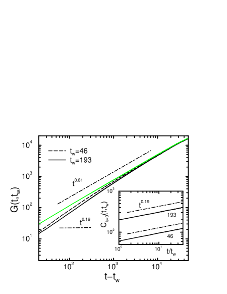
FIG. 1.: $G(t,t_{w})$ vs $t-t_{w}$ for two different waiting times $t_{w}=46$ and $193$. The grey line is the leading waiting time independent contribution $C_{k=0}(t,t)$ which grows in time with a power-law with an exponent $(d-2\beta/\nu)/z\approx 0.81$. Systems with $300\times 300$ spins have been simulated, and all the data shown in the present work have been averaged over 70000 different runs. The inset shows that the ageing part $C_{k=0}(t,t_{w})$ of $G(t,t_{w})$ indeed grows as $t^{0.19}$, as predicted by scaling arguments.

To compute the susceptibility of the magnetization a small homogeneous constant field of strength $h$ is switched on after the waiting time $t_{w}$ [1]. The integrated susceptibility is then given by [7]

$$\chi_{m}(t,t_{w})=\frac{T_{c}}{N\,h}\langle\sum\limits_{i=1}^{N}s_{i}\rangle=\frac{T_{c}}{h}m.$$ (10)

The magnetization $m$ is measured for times $t>t_{w}$ and depends both on $t$ and $t_{w}$. Starting from an uncorrelated initial state, the dynamical correlation length increases with time, $\xi(t)\sim t^{1/z}$, up to $t_{w}$. The homogeneous external field, which is applied for times $t\geq t_{w}$, drives the system away from the critical point towards a new equilibrium point located at $T=T_{c}$ and $m=m_{final}>0$. This new equilibrium point is reached at finite times, independently of the waiting time. This is also the case when the system is already in equilibrium at the critical point and an homogeneous external field is then switched on. One therefore expects that the extension of the correlated regions (and therefore the value of $t_{w}$) is only of importance for a short period after the application of the field, but that at later times the system looses the memory of the value of $\xi(t_{w})$, thus that $\chi_{m}(t,t_{w})$ approaches $\chi_{FC}(t):=\chi_{m}(t,0)$ for all waiting times. Here, $\chi_{FC}(t)$ is the field cooling susceptibility. This is illustrated in Fig. 2 where the field strength $h=0.0004$ is the same as that used by MBGS [12]. One indeed observes that the curves with $t_{w}\neq 0$ rapidly approach the curve for $t_{w}=0$. Note that the plateau reached at longer times is not a finite-size effect, but is due to the new equilibrium point. One further remarks from Fig. 2 that $\chi_{FC}(t)$ exhibits a power-law behaviour. The value of the corresponding exponent can be obtained from the standard dynamical scaling relation for $m$ [9] (with $m(t=0)=0$)

$$m(t,\tau,h)=b^{-\beta/\nu}\,m(b^{-z}\,t,b^{1/\nu}\,\tau,b^{d-\beta/\nu}\,h)$$ (11)

where $\tau$ is the reduced temperature. In our case $\tau=0$ as the temperature is fixed at $T_{c}$ after the quench. Setting $b=t^{1/z}$ one gets

$$m(t,h)=t^{-\beta/\nu z}\,m(1,t^{(d-\beta/\nu)/z}\,h)$$ (12)

and

$$\chi_{FC}(t)=\frac{T_{c}}{h}m(t,h)\sim t^{(d-2\beta/\nu)/z}$$ (13)

where the last step $h$ is valid for $t\ll h^{-(d-\beta/\nu)/z}$. This expected power-law behaviour is also shown in Fig. 2. It is important to note that $\chi_{FC}(t)$ increases with the same exponent $(d-2\beta/\nu)/z$ as the leading contribution $C_{k=0}(t,t)$ of the correlation $G(t,t_{w})$, and this already after a few time steps.

 

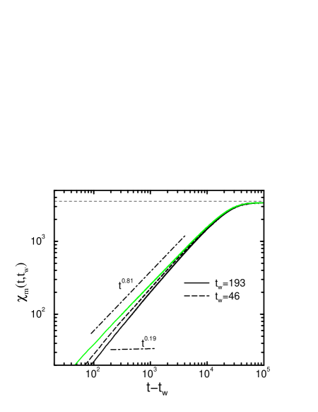
FIG. 2.: The susceptibilty of the magnetization $\chi_{m}(t,t_{w})$ as function of the time $t-t_{w}$ elapsed since the switching on of the homogeneous constant external field. One observes that the curves for waiting times $t_{w}\neq 0$ rapidly converge to the curve obtained for $t_{w}=0$ where the system is quenched to $T_{c}$ in presence of the field. The leading contribution of the susceptibility also grows with a power-law with an exponent $(d-2\beta/\nu)/z\approx 0.81$. The thin dashed line indicates the final value of $\chi_{m}(t,t_{w})$ at the new equilibrium point.

As the leading non-ageing contributions of both quantities used by MBGS display the same power-law behaviour, one may wonder whether the straight lines observed in their fluctuation-dissipation plots, Figs. 8 and 10 in [1], are not simply due to this non-ageing parts. From the scaling arguments one expects that the ratio $\chi_{m}(t,t_{w})/G(t,t_{w})$ is given by $\chi_{m}(t,t_{w})/G(t,t_{w})=\chi_{FC}(t)/C_{k=0}(t,t)+O(t^{2\beta/\nu z-\lambda_{c}/z})$ with $2\beta/\nu z-\lambda_{c}/z=-0.62$ for the two-dimensional Ising model. The ratio $\chi_{FC}(t)/C_{k=0}(t,t)$ is expected to take a constant value $\overline{X}$ already after a few time steps. This is indeed the case, as shown in Fig. 3. Here I plot $\chi_{FC}(t)$ as function of $C_{k=0}(t,t)$ and compare the resulting line with those obtained when plotting $\chi_{m}(t,t_{w})$ as function of $G(t,t_{w})$ for $t_{w}=46$ and $193$, as done by MBGS. The behaviour of these quantities at the very first time steps is displayed in the inset. It is now obvious why MBGS obtain straight lines with a constant slope for any value of the waiting time $t_{w}$: the ageing (i.e. waiting time dependent) parts are rapidly suppressed in this kind of plot and the slope is then identical to the slope obtained from two quantities which do not depend on the waiting time and which furthermore have the same time dependence.

 

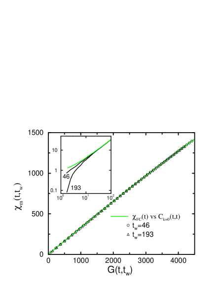
FIG. 3.: Fluctuation-dissipation plot similar to Fig. 8 in [1] for waiting times $t_{w}=46$ and $193$. Only every 200th data point is shown. The grey line is the correponding curve obtained from plotting the leading waiting time independent contribution $\chi_{FC}(t)=\chi_{m}(t,0)$ of the susceptibility as function of the leading waiting time independent contribution $C_{k=0}(t,t)$ of $G(t,t_{w})$. Obviously, the slopes of the different curves are identical after very few time steps and are exclusively due to the non-ageing parts of the different quantities, see inset.

In conclusion I have shown that the leading terms of the integrated quantities used in [1] for the numerical determination of the fluctuation-dissipation ratios are independent of the waiting time. I have also shown that the leading terms of the correlation (9) and the susceptibility (10) grow in time with the same power-law. This explains why MBGS observe in their fluctuation-dissipation plots straight lines with a constant slope that does neither depend on the waiting time $t_{w}$ nor on the observation time $t$.

It is a pleasure to thank A. Gambassi for interesting discussions which led to the present study, and A. Gambassi and M. Henkel for a critical reading of the manuscript. This work was supported by the Bayerisch-Französisches Hochschulzentrum (BFHZ) and by CINES Montpellier (projet pmn2095). Some simulations have also been done on the IA32 cluster of the Regionales Rechenzentrum Erlangen (RRZE). I thank G. Hager of the HPC-team of RRZE for technical assistance.

REFERENCES

- [1] P. Mayer, L. Berthier, J.P. Garrahan, and P. Sollich, Phys. Rev. E 68, 016116 (2003).
- [2] C. Godrèche and J.M. Luck, J. Phys. Condens. Matter 14, 1589 (2002).
- [3] L.F. Cugliandolo, in Slow Relaxation and non equilibrium dynamics in condensed matter, Les Houches Session 77 July 2002, J-L Barrat, J Dalibard, J Kurchan, M V Feigel’man eds (Springer, 2003).
- [4] MBGS also studied energy related quantities. For simplicity, I will only discuss the spin-spin correlation function and the conjugate response function. The criticism formulated in this comment also applies to the energy related quantities.
- [5] P. Calabrese and A. Gambassi, Phys. Rev. E 66, 066101 (2002).
- [6] H.K. Janssen, B. Schaub, and B. Schmittmann, Z. Phys. B 73, 539 (1989).
- [7] The quantities here are the same as those used by MBGS.
- [8] U. Ritschel and H.W. Diehl, Nucl. Phys. B464, 512 (1996).
- [9] K. Okano, L. Schülke, K. Yamagishi, and B. Zheng, Nucl. Phys. B485, 727 (1997).
- [10] I only consider the case where . In the presence of an initial magnetization , the expression for has to be slightly modified, see [8].
- [11] C. Yeung, M. Rao, and R.C. Desai, Phys. Rev. E53, 3073 (1996).
- [12] L. Berthier, private communication.