Bifurcation analysis in an associative memory model

Abstract

We previously reported the chaos induced by the frustration of interaction in a non-monotonic sequential associative memory model, and showed the chaotic behaviors at absolute zero. We have now analyzed bifurcation in a stochastic system, namely a finite-temperature model of the non-monotonic sequential associative memory model. We derived order-parameter equations from the stochastic microscopic equations. Two-parameter bifurcation diagrams obtained from those equations show the coexistence of attractors, which do not appear at absolute zero, and the disappearance of chaos due to the temperature effect.

I Introduction

Chaos occurs in systems that consist of chaotic or binary units. For instance, the globally coupled map and chaos neural networks Kaneko1989 ; Aihara1990 ; Adachi1997 ; Shibata1998 consist of chaotic units, while neural networks consist of non-chaotic units. Although the processing units in neural networks are simple binary units, chaotic behavior can be observed at the macroscopic level. Chaotic behavior can be induced by various mechanisms: synaptic pruning, synaptic delay, thermal noise, sparse connections, and/or so on FukaiShiino1990 ; Nara1992 ; vanVreeswijk ; Kawamura2003 . These models are deterministic systems. Chaotic behavior can also be observed in stochastic systems Tsuda1992 . Using the Dale hypothesis, Fukai and Shiino FukaiShiino1990 showed that chaos can occur in neural networks.

Stochastic behavior can be distinguished from chaotic behavior based on the exponents, e.g., the Lyapunov exponent. Therefore, analyzing deterministic chaos in stochastic systems is very interesting MatsumotoTsuda1983 ; ShibataChawanyaKaneko1999 . While there is a close relationship between microscopic behavior and macroscopic behavior, the macroscopic state cannot always be estimated from the microscopic state. Frustration-induced chaos is an example of that. For continuous systems, chaotic behaviors in some small networks with frustration of interaction can be analyzed at the microscopic level Bersini1995 ; Bersini1998 ; Bersini2002 . In some large random neural networks, a dynamical mean-field theory was introduced to analyze chaotic behaviors by Sompolinsky et al. Sompolinsky1988 . We have shown that chaos can be induced by frustration of interaction in a non-monotonic sequential associative memory model Kawamura2003 .

The sequential associative memory model is a neural network in which the sequence of patterns is embedded as an attractor through Hebbian (correlation) learning Amari1988 ; During1998 ; Katayama2001 ; Kawamura2002 . When the number of patterns, $p$, is of the order ${\cal O}(N)$, where $N$ is the number of processing units, the model has frustrated interactions Rieger1998 . The properties in stationary states were analyzed exactly using the path-integral method During1998 ; Katayama2001 because the theoretical treatment of the transient was difficult. However, the transient of the model was recently rigorously analyzed Kawamura2002 .

The non-monotonicity of processing units (a larger absolute value of the local field tends to make their state opposite that of the local field) gives a system superior properties, e.g., enhanced storage capacity, fewer spurious states, and a super retrieval phase Morita1993 ; ShiinoFukai1993 ; Okada1996 . The systems with non-monotonic units have chaotic behaviors. Dynamic theories are indispensable for analyzing the chaotic behaviors. The dynamical mean-field theory Sompolinsky1988 is exact in the limit of $N\to\infty$, and one can analyze the chaotic behaviors in random neural networks. Only approximated theories, e.g., Gaussian approximation Amari1988 ; Okada1996 ; AmariMaginu1988 ; NishimoriOpris1993 ; Okada1995 ; Kawamura1999 or steady-state approximation During1998 ; Katayama2001 , have been used to investigate the occurrence of these chaotic behaviors in the associative memory models.

In our previous work Kawamura2003 , we constructed bifurcation diagrams of a non-monotonic system. We showed chaotic behaviors in a non-monotonic sequential associative memory model at absolute zero and demonstrated that the chaos occurs only when it has some degree of frustration.

In this paper, we analyze bifurcations in our model at a finite temperature. We note that the microscopic behavior is stochastic while the macroscopic one is deterministic Kawamura2002 . We can therefore analyze its macroscopic dynamics rigorously and construct two-parameter bifurcation diagrams from our order-parameter equations. The structure of the bifurcation is changed by the finite temperature effect. We analytically show the area of a cusp point and the coexistence of attractors, which do not appear at absolute zero.

II Sequential associative memory model

Consider a sequential associative memory model consisting of $N$ units or neurons. The state of the units takes $\sigma_{i}(t)=\pm 1$ and is updated synchronously with probability

$$\mbox{Prob}\left[\sigma_{i}(t+1)|h_{i}(t)\right]=\frac{1}{2}\left[1+\sigma_{i}(t+1)F\left(h_{i}(t)\right)\right],$$ (1)

$$h_{i}(t)=\sum_{j=1}^{N}J_{ij}\sigma_{j}(t)+I_{i}(t),$$ (2)

where $J_{ij}$ is the coupling, $I_{i}(t)$ is the threshold or external input, and $h_{i}(t)$ is the local field. Function $F\left(h\right)$ is a non-monotonic function given by

$$F\left(h\right)=\tanh\beta h-\tanh\beta\left(h-\theta\right)-\tanh\beta\left(h+\theta\right),$$ (3)

where $\beta$ is the inverse temperature ($\beta=1/T$), and $\theta$ is the non-monotonicity. When $T=0$, the update rule of the model is deterministic:

$$\sigma_{i}(t+1)=\mbox{sgn}\left(h_{i}(t)\right)-\mbox{sgn}\left(h_{i}(t)-\theta\right)-\mbox{sgn}\left(h_{i}(t)+\theta\right).$$ (4)

When the absolute value of the local field is larger then $\theta$, the sign of the state is opposite that of the local field, i.e., $\sigma_{i}(t+1)=-\mbox{sgn}\left(h_{i}(t)\right)$. Coupling $J_{ij}$ stores $p$ random patterns, $\mbox{\boldmath$\xi$}^{\mu}=(\xi^{\mu}_{1},\cdots,\xi^{\mu}_{N})^{T}$, so as to retrieve the patterns sequentially: $\mbox{\boldmath$\xi$}^{0}\to\mbox{\boldmath$\xi$}^{1}\to\cdots\mbox{\boldmath$\xi$}^{p-1}\to\mbox{\boldmath$\xi$}^{0}$. It is given by

$$J_{ij}=\frac{1}{N}\sum_{\mu=0}^{p-1}\xi^{\mu+1}_{i}\xi^{\mu}_{j},$$ (5)

where $\mbox{\boldmath$\xi$}^{p}=\mbox{\boldmath$\xi$}^{0}$. The number of stored patterns is given by $p=\alpha N$, where $\alpha$ is the loading rate. Each component of the patterns is assumed to be an independent random variable that takes a value of either $+1$ or $-1$ based on

$$\mbox{Prob}\left[\xi_{i}^{\mu}=\pm 1\right]=\frac{1}{2}.$$ (6)

We determine the initial state, $\mbox{\boldmath$\sigma$}(0)$, based on

$$\mbox{Prob}[\sigma_{i}(0)=\pm 1]=\frac{1\pm m(0)\xi^{0}_{i}}{2}.$$ (7)

The overlap, the direction cosine between $\mbox{\boldmath$\sigma$}(0)$ and $\mbox{\boldmath$\xi$}^{0}$, converges to $m(0)$ as $N\to\infty$.

III Macroscopic state equations

To discuss the transient, we introduce macroscopic state equations by using the path-integral method During1998 ; Katayama2001 ; Kawamura2002 . Generating function $Z[\mbox{\boldmath$\psi$}]$ is defined as

$$Z[\mbox{\boldmath$\psi$}] = \sum_{\mbox{\boldmath$\sigma$}(0),\cdots,\mbox{\boldmath$\sigma$}(t)}p\left[\mbox{\boldmath$\sigma$}(0),\mbox{\boldmath$\sigma$}(1),\cdots,\mbox{\boldmath$\sigma$}(t)\right]\exp\left(-i\sum_{s<t}\mbox{\boldmath$\sigma$}(s)\cdot\mbox{\boldmath$\psi$}(s)\right),$$ (8)

where $\mbox{\boldmath$\psi$}=\left(\mbox{\boldmath$\psi$}(0),\cdots,\mbox{\boldmath$\psi$}(t-1)\right)$. State $\mbox{\boldmath$\sigma$}(s)=(\sigma_{1}(s),\cdots,\sigma_{N}(s))^{T}$ denotes the state of the spins at time $s$, and path probability $p\left[\mbox{\boldmath$\sigma$}(0),\mbox{\boldmath$\sigma$}(1),\cdots,\mbox{\boldmath$\sigma$}(t)\right]$ denotes the probability of taking the path from initial state $\mbox{\boldmath$\sigma$}(0)$ to state $\mbox{\boldmath$\sigma$}(t)$ at time $t$ through $\mbox{\boldmath$\sigma$}(1),\mbox{\boldmath$\sigma$}(2),\cdots,\mbox{\boldmath$\sigma$}(t-1)$. Since the dynamics, eq. (1), is a Markov chain, the path probability is given by

$$p\left[\mbox{\boldmath$\sigma$}(0),\mbox{\boldmath$\sigma$}(1),\cdots,\mbox{\boldmath$\sigma$}(t)\right]=p\left[\mbox{\boldmath$\sigma$}(0)\right]\prod_{s<t}\prod_{i}\frac{1}{2}\left[1+\sigma_{i}(s+1)F\left(h_{i}(s)\right)\right].$$ (9)

The generating function involves the following order parameters:

$$m(s) = i\lim_{\mbox{\boldmath$\psi$}\to 0}\frac{1}{N}\sum_{i=1}^{N}\xi_{i}^{s}\frac{\partial Z[\mbox{\boldmath$\psi$}]}{\partial\psi_{i}(s)},$$ (10)

$$G(s,s^{\prime}) = i\lim_{\mbox{\boldmath$\psi$}\to 0}\frac{1}{N}\sum_{i=1}^{N}\frac{\partial^{2}Z[\mbox{\boldmath$\psi$}]}{\partial\psi_{i}(s)\partial I_{i}(s^{\prime})},$$ (11)

$$C(s,s^{\prime}) = -\lim_{\mbox{\boldmath$\psi$}\to 0}\frac{1}{N}\sum_{i=1}^{N}\frac{\partial^{2}Z[\mbox{\boldmath$\psi$}]}{\partial\psi_{i}(s)\partial\psi_{i}(s^{\prime})}.$$ (12)

Order parameter $m(s)$ corresponds to the overlap, which represents the direction cosine between state $\mbox{\boldmath$\sigma$}(s)$ and retrieval pattern $\mbox{\boldmath$\xi$}^{s}$ at time $s$. $G(s,s^{\prime})$ and $C(s,s^{\prime})$ are the response and correlation functions, respectively, between time $s$ and $s^{\prime}$. Therefore, the problem of evaluating the macroscopic dynamics leads to the problem of evaluating the generating function.

We consider the case of thermodynamic limit $N\to\infty$ and analyze $Z[\mbox{\boldmath$\psi$}]$ using the saddle point method. Since $N\to\infty$ and stored patterns $\mbox{\boldmath$\xi$}^{\mu}$ are random patterns, we can assume self-averaging with respect to the realization of disorder; that is, we would like to average $Z[\mbox{\boldmath$\psi$}]$ over the uncondensed patterns. And then using the normalization condition $Z\left[0\right]=1$ DominicisPeliti1978 ; Dominicis1978 , we can eliminate invalid order parameters and derive effective order parameters. We can therefore obtain a rigorous solution using the path-integral method Kawamura2002 .

Finally, we obtain the following macroscopic state equations from $Z[\mbox{\boldmath$\psi$}]$ when $I_{i}(s)=0$:

$$m(s) = \left<\xi^{s}\int D_{z}F\left(\xi^{s}m(s-1)+z\sqrt{\alpha R(s-1,s-1)}\right)\right>_{\xi},$$ (13)

$$R(s,s^{\prime}) = C(s,s^{\prime})+G(s,s-1)G(s^{\prime},s^{\prime}-1)R(s-1,s^{\prime}-1),$$ (14)

$$G(s,s-1) = \frac{1}{\sqrt{\alpha R(s-1,s-1)}}$$ (15)

$$\times \left<\int\!D_{z}zF\left(\xi^{s}m(s-1)+z\sqrt{\alpha R(s-1,s-1)}\right)\!\right>_{\xi},$$

$$C(s,s^{\prime}) = \left<\int\frac{d\mbox{\boldmath$z$}}{2\pi|\mbox{\boldmath$R$}_{11}|^{\frac{1}{2}}}\exp\left[-\frac{1}{2}\mbox{\boldmath$z$}\cdot\mbox{\boldmath$R$}_{11}^{-1}\mbox{\boldmath$z$}\right]F\left(\xi^{s}m(s-1)+\sqrt{\alpha}z(s-1)\right)\right.$$ (16)

$$\left.\times F\left(\xi^{s^{\prime}}m(s^{\prime}-1)+\sqrt{\alpha}z(s^{\prime}-1)\right)\right>_{\xi},$$

where $D_{z}=\frac{dz}{\sqrt{2\pi}}\exp[-\frac{1}{2}z^{2}]$, and $\left<\cdot\right>_{\xi}$ denotes the average over all $\xi$’s. Matrix $\mbox{\boldmath$R$}_{11}$ is a $2\times 2$ matrix consisting of the elements of $R$ at times $s-1$ and $s^{\prime}-1$, and $\mbox{\boldmath$z$}=[z(s-1),z(s^{\prime}-1)]^{T}$. From eqs. (13)–(16), $C(s,s^{\prime})=0$ and $R(s,s^{\prime})=0$ when $s\neq s^{\prime}$. Since $G(s,s-1)$ and $C(s,s)$ can be described using only $m(s-1)$ and $R(s-1,s-1)$, macroscopically this system is a two-degree-of-freedom system of $m(s)$ and $R(s,s)$. Since we can easily calculate the Gaussian integrals, we can analyze the transient dynamics exactly even if the network fails in retrieval. We note that $m(s)$ is an odd function and $R(s,s)$ is an even function, since the function $F(h)$ is an odd function. Therefore, the map by the macroscopic state equations is line symmetric with respect to the line $m=0$.

Besides these dynamic macroscopic state equations, the fixed points of the system are required in order to analyze the bifurcation of the system. We set $m(t)\to m,G(t,t-1)\to G$ and $R(t,t)\to r$ when $t\to\infty$. Then, the previously obtained stationary state equations During1998 ; Katayama2001 are re-derived using our dynamic theory:

$$m = \left<\xi\int D_{z}F\left[\xi m+z\sqrt{\alpha r}\right]\right>_{\xi},$$ (17)

$$G = \frac{1}{\sqrt{\alpha r}}\left<\int D_{z}zF\left[\xi m+z\sqrt{\alpha r}\right]\right>_{\xi},$$ (18)

$$r = \frac{1}{1-G^{2}}.$$ (19)

IV Macroscopic dynamics

We can obtain the macroscopic dynamics (13)–(16) from the stochastic microscopic dynamics. Moreover, the Jacobian matrix, $\mbox{\boldmath$J$}(s)$, can be easily calculated from these equations:

$$\mbox{\boldmath$J$}(s)=\left[\begin{array}[]{cc}\frac{\partial m(s)}{\partial m(s-1)}&\frac{\partial m(s)}{\partial R(s-1,s-1)}\\ \frac{\partial R(s,s)}{\partial m(s-1)}&\frac{\partial R(s,s)}{\partial R(s-1,s-1)}\end{array}\right].$$ (20)

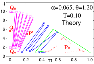
(a) (b)

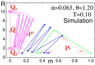
Figure 1: Transition of overlap $m(t)$ and variance of crosstalk noise $\alpha R(t,t)$ for $\alpha=0.065,\theta=1.20,T=0.10$. Fixed points $P,P^{\prime},Q$ are from stationary state equations: (a) our theory, (b) simulation ($N=100,000$).

We can therefore classify fixed points according to their eigenvalues, $\lambda$. We analyze the transient for a finite temperature, e.g., $T=0.10$. Figure 1 shows the transition of the overlap, $m(t)$, and the variance of the crosstalk noise, $\alpha R(t,t)$. The graphs show the results obtained using (a) our theory and (b) computer simulation with $N=100,000$, where loading rate $\alpha$ is $0.065$ and non-monotonicity $\theta$ is $1.20$. The cross marks ($P,P^{\prime},Q$) are fixed points. Point $P$ is a repellor (unstable focus), since the eigenvalues are $\lambda=-0.21\pm 1.40i$; $P^{\prime}$ is a repellor (unstable node) because $\lambda=-1.30,1.18$; and $Q$ on line $m=0$ is a saddle node (orientation reversing) because $\lambda=-1.29,0.91$. There is a period-$2$ attractor, $Q_{2}$, that attracts the trajectories with initial state $m(0)\approx 0$. Moreover, there is a chaotic attractor around repellor $P$. The results obtained using our theory agree with those using computer simulation. Since our dynamic macroscopic state equations are derived exactly, the difference between the theoretical analysis and the computer simulation is due to finite size effect.

V Bifurcation diagram for $T=0$

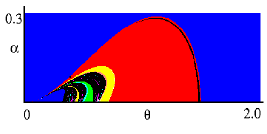
(b)

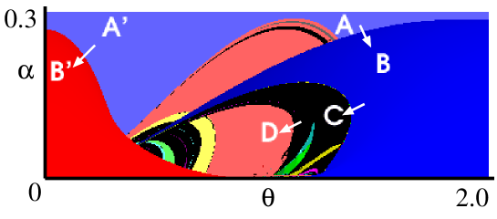
Figure 2: Two-parameter bifurcation diagram ($\theta,\alpha$) for (a) fixed point $Q$ and (b) fixed point $P$ at $T=0$. Blue region represents period-$1$ attractors, red period-$2$, green period-$3$, yellow period-$4$, purple period-$5$, sky blue period-$6$, and black for more than six periods, quasi-periodic or chaotic.

We investigated the relationships of the invariant sets shown in Fig. 1 in two-parameter space with respect to $(\theta,\alpha)$. Line $m=0$ is an invariant set of the macroscopic state equations, and the map of the system is line symmetric with respect to invariant line $m=0$, as stated above. The dynamic structure on this invariant line obeys a one-dimensional map with respect to $R(t,t)$ Kawamura2003 . Figure 2 (a) shows a two-parameter bifurcation diagram for the attractor on invariant line $m=0$, and (b) shows one for the attractor around repellor $P$ for $T=0$. The blue region represents the period-$1$ attractors, red period-$2$, green period-$3$, yellow period-$4$, purple period-$5$, sky blue period-$6$, and black for more than six periods, quasi-periodic or chaotic. In Fig. (a), as $\theta$ decreases, a period-$1$ attractor, $Q$, bifurcates to a period-$2$ attractor, $Q_{2}$, and evolves into a chaotic attractor due to the period-doubling cascade. In Fig. (b), some regions are denoted by $A,A^{\prime},B,B^{\prime},C,$ and $D$, and we can find bifurcations on the boundaries between these regions.

V.1 Transient

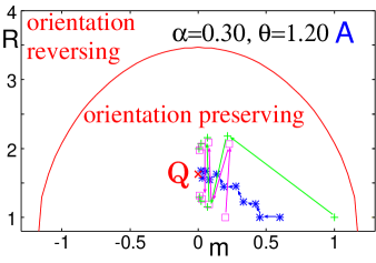
(a) (b)

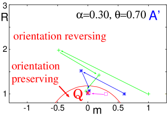
Figure 3: Attractor $Q$ in (a) region $A$ ($\alpha=0.30,\theta=1.20$) and (b) region $A^{\prime}$ ($\alpha=0.30,\theta=0.70$) at $T=0$ by our theory. Area inside semielliptic arc is orientation-preserving area, and area outside is orientation-reversing area.

Figure 3 shows the transient in regions $A$ and $A^{\prime}$. There is only a period-$1$ attractor, $Q$, on the invariant line. Since the map by our macroscopic state equations is irreversible, there is an orientation-preserving area inside the semielliptical arc, and an orientation-reversing area outside the arc. The orientation-preserving area shrinks as $\theta$ decreases. Therefore, the transient in $A$ differs from that in $A^{\prime}$. In both cases, since the stored patterns are unstable, the associative memory fails to retrieve one from any initial state.

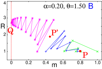
(a) (b)

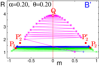
Figure 4: Attractors $P$ and $P_{2}$ in (a) region $B$ ($\alpha=0.20,\theta=1.50$) and (b) region $B^{\prime}$ ($\alpha=0.20,\theta=0.20$) at $T=0$ by our theory.

Figure 4 shows the transient in regions $B$ and $B^{\prime}$. In region $B$, there is both a period-$1$ attractor, $Q$, on the invariant line and a period-$1$ attractor, $P$, near $m=1$. The orientation-reversing area is far from the origin. In this case, since the stored patterns are stable, the associative memory can retrieve one when the state is in the basin of the attraction of $P$. Additionally, in region $B^{\prime}$, there is both attractor $Q$ and period-$2$ attractor $P_{2}$. The orientation-preserving area shrinks to near the origin. Attractor $P_{2}$ is a sign-reversing state near line $m=\pm 1$. In this case, the stored patterns are unstable, and the memory retrieves the stored pattern and its reverse one in turn when the state is in the basin of attraction of $P_{2}$.

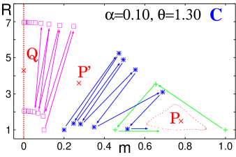
(a) (b)

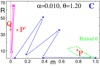
(c)

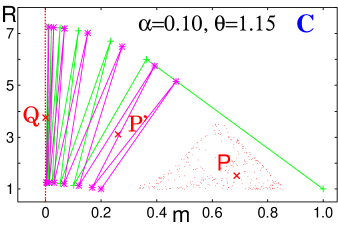
Figure 5: Attractors around $P$ in region $C$: (a) quasi-periodic attractor ($\alpha=0.10,\theta=1.30$), (b) period-$6$ attractor ($\alpha=0.01,\theta=1.20$), and (c) chaotic attractor ($\alpha=0.10,\theta=1.15$).

Figure 5 shows the transient in region $C$. There is both a period-$2$ attractor, $Q_{2}$, on the invariant line and a certain attractor near $m=1$. The attractor around repellor $P$ is periodic, quasi-periodic, or chaotic. In this case, although the stored patterns are unstable, there is a quasi-periodic or chaotic attractor. The state, therefore, goes to this attractor instead of the memory state. Since the overlap is non-zero, the associative memory neither completely succeeds nor fails to retrieve patterns.

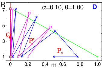
Figure 6: Attractors around $P$ in region $D$ ($\alpha=0.10,\theta=1.00$) vanish due to boundary crisis.

Figure 6 shows the transient in region $D$. There is a period-$1$ attractor, $Q$, and a period-$2$ attractor, $Q_{2}$, on the invariant line. In this case, since the stored patterns are unstable, the associative memory fails to retrieve one from any initial state.

V.2 Bifurcations

The coexistence, as stated above, can be explained by the occurrence of characteristic bifurcations on the boundary between regions. On boundary $A\to B$, saddle node $P^{\prime}$ and period-$1$ attractor $P$ are generated by the saddle node bifurcation, leading to the existence of both $Q$ and $P$. They are separated by the basin boundary constituted by $P^{\prime}$. The boundary $B\to A$ represents the storage capacity, i.e., the critical loading rate. On boundary $A^{\prime}\to B^{\prime}$, similarly, period-$2$ saddle node $P_{2}^{\prime}$ and period-$2$ attractor $P_{2}$ are generated by the saddle node bifurcation, leading to the existence of both $Q$ and $P_{2}$. In contrast, on boundary $B\to C$, period-$1$ attractor $P$ evolves into a repellor due to the Hopf bifurcation, and a quasi-periodic attractor is generated around the repellor. This attractor is sometimes phase-locked, and then it evolves into a more complex quasi-periodic attractor by the Hopf bifurcation again. The repellor inside the quasi-periodic attractor then evolves into a snap-back repellor Marotte1978 , and belt-like chaos appears. Finally, the chaos spreads and becomes a thick chaotic attractor, including repellor $P$. On boundary $C\to D$, the chaotic attractor disappears due to a boundary crisis Grebogi1982 because it comes into contact with the basin boundary constituted by $P^{\prime}$. Therefore, in region $D$, there is only period-$2$ attractor $Q_{2}$ on the invariant line.

VI Bifurcation diagram for $T>0$

We constructed two-parameter bifurcation diagrams for several finite temperatures. Figure 7 shows the diagrams for an attractor on invariant line $m=0$ for $T=0.0-0.35$. The abscissa denotes $\theta$ ($0<\theta<1.7$), and the ordinate denotes $\alpha$ ($0<\alpha<0.302$) on a logarithmic scale. In the center of the diagrams, we can find another bistable region in which attractors coexist. As the temperature is increased, the bistable region becomes larger. For $T>0$, there is a fishhook structure where the region of each periodic attractor divides into two regions. When $T\geq 0.30$, the more-than-two-period attractors and chaotic attractors disappear.

Figure 8 shows the two-parameter bifurcation diagrams for fixed point $P$ or of the attractors around $P$ for $T=0.0-0.40$. The diagrams overlay those in Fig. 7 since one can see the coexistence of attractors $P$ and $Q$. As the temperature is increased, the Hopf bifurcation set becomes an isolated circle and disappears via the codimension-$2$ bifurcation set. Since a fishhook structure is evident in the diagram, there is a cusp point, i.e., a codimension-$2$ bifurcation set, which generates a pair of saddle node bifurcation sets.

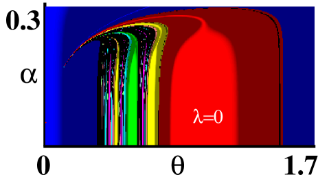
(a) $T=0$

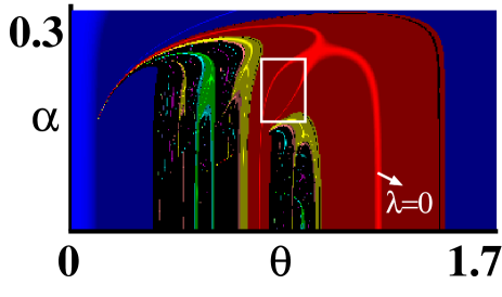
(b) $T=0.05$

Figure 9: Curve of eigenvalue $\lambda=0$ and area of cusp point for (a) $T=0$ and (b) $T=0.05$. Cusp point is in rectangular area.

We show the region where the cusp point exists. Figure 9 shows the two-parameter bifurcation diagrams for fixed point $Q$, which are graded by eigenvalue $\lambda$. The bright lines denote eigenvalue $\lambda=0$. There is only one curve for $\lambda=0$ at $T=0$, whereas there are two for $T=0.05$. A cusp point is in the region surrounded by the curves.

VII Discussion

We can see that the chaotic region may be expanding to $\alpha\to 0$ in Figs. 7 and 8. We first discuss the cases of $\alpha=0$ and $\alpha\to 0$. Only one order-parameter, $m(t)$, dominates the macroscopic behaviors of the present system without frustration of interaction, that is, when the number of stored patterns is finite ($\alpha=0$). We can easily show that there is no chaotic attractor in this case. A chaotic attractor appears when the system has frustration, i.e., $\alpha\neq 0$. While the local field, $h_{i}(t)$, obeys a $\delta$-function distribution when $\alpha=0$, it obeys a Gaussian distribution with variance $\alpha R(t,t)$ when $\alpha\neq 0$. We show the simple case of $T=0$ and $m(t)=0$. From eqs. (4), (14), and (15), the variance of crosstalk noise, $\alpha R(t+1,t+1)$, can be given by

$$\alpha R(t+1,t+1) = \alpha+\frac{2}{\pi}\left\{1-2\exp\left(-\frac{\theta^{2}}{2\alpha R(t,t)}\right)\right\}^{2}.$$ (21)

When $\alpha\to 0$, $\alpha R(t+1,t+1)$ converges to

$$\alpha R(t+1,t+1)=\frac{2}{\pi}\left\{1-2\exp\left(-\frac{\theta^{2}}{2\alpha R(t,t)}\right)\right\}^{2},$$ (22)

since $R(t,t)$ takes a large value in inverse proportion to $\alpha$. That is, $\alpha R(t+1,t+1)$ still takes a finite value even if $\alpha\to 0$. Figure 10 shows the return map of $\alpha R(t,t)$ for $T=0$ and $0.3$. We can see that the fixed point is finite ($\alpha R(t,t)>0$). Because of this finite variance of the local field distribution, the processing units, whose absolute values of local field $h_{i}(t-1)$ are around non-monotonicity $\theta$, take different values, similar to those in Bakers’ Map. This is the reason for the occurrence of chaos in this model with frustration. Non-trivial findings are that chaos also appears when $\alpha\to 0$ and that the phase is completely different from when $\alpha=0$.

Next we discuss the reason for the change in the bifurcation structure due to the finite temperature effect. We consider the case of an attractor on $m(t)=0$. Since fixed point $Q$ is on invariant line $m=0$, the dynamics obeys a one-dimensional map with respect to $R(t,t)$. Figure 11 shows the return map of $R(t,t)$. For $T=0$ (solid line), the map is unimodal and there is a period-$2$ attractor, whereas the map is bimodal and there is a period-$4$ attractor for $T=0.1$ (broken line). Therefore, the finite temperature effect changes the bifurcation structure, causing a bistable region to appear. When $T$ is large enough, the more-than-two-period attractors and chaotic attractors disappear. Thermal noise, therefore, orders the system. The ordering mechanism may be similar to that of noise-induced order MatsumotoTsuda1983 ; ShibataChawanyaKaneko1999 .

In summary, we considered a sequential associative memory model consisting of non-monotonic units, which is a stochastic system, and derived macroscopic state equations using the path-integral method in the frustrated case. The results obtained by theory agreed with the results obtained by computer simulation. We constructed two-parameter bifurcation diagrams for various temperatures and used them to explain the changes in the structure of the bifurcations caused by the temperature effect and the coexistence of attractors.

(a)

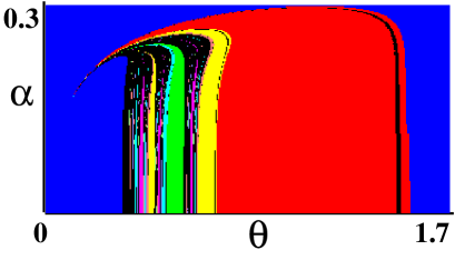
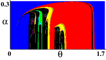
(a) $T=0$ (b) $T=0.05$

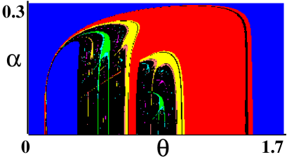
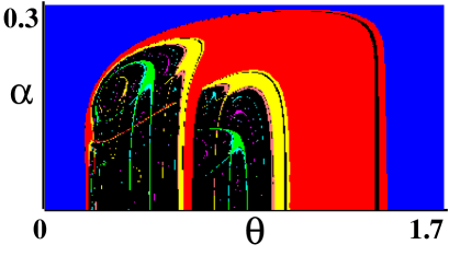
(c) $T=0.10$ (d) $T=0.15$

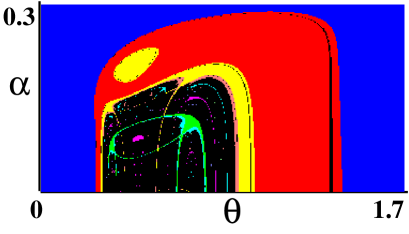
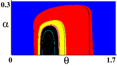
(e) $T=0.20$ (f) $T=0.25$

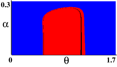
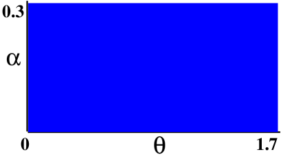
(g) $T=0.30$ (h) $T=0.35$

Figure 7: Two-parameter bifurcation diagrams on invariant line $m=0$ for (a) absolute zero ($T=0$) and (b)–(h) finite temperature ($T=0.05-0.35$). Abscissa denotes $\theta$ ($0<\theta<1.7$), and ordinate denotes $\alpha$ ($0<\alpha<0.302$) on logarithmic scale. Colors denote period of attractors as in Fig. 2.

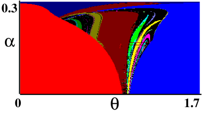
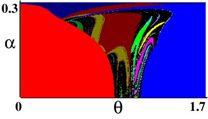
(a) $T=0$ (b) $T=0.05$

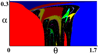
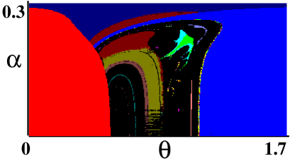
(c) $T=0.15$ (d) $T=0.25$

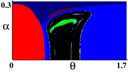
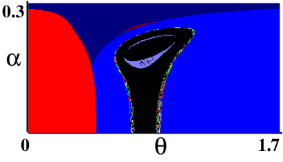
(e) $T=0.30$ (f) $T=0.32$

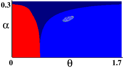
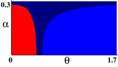
(g) $T=0.35$ (h) $T=0.40$

Figure 8: Two-parameter bifurcation diagrams around fixed point $P$ for (a) absolute zero ($T=0$) and (b)–(h) finite temperature ($T=0.05-0.40$). Abscissa denotes $\theta$ ($0<\theta<1.7$), and ordinate denotes $\alpha$ ($0<\alpha<0.302$) on logarithmic scale. Colors denote period of attractors as in Fig. 2.

Figure 10: Return map of variance of crosstalk noise, $\alpha R(t,t)$ for $\alpha=0.001,\theta=1.0$. Solid and broken lines denote cases of $T=0$ and $T=0.3$, respectively.

Figure 11: Return map of $R(t,t)$ for $\alpha=0.01,\theta=0.8$. Solid and broken lines denote cases of $T=0$ and $T=0.1$, respectively.

References

- (1) K. Kaneko, Chaotic but regular posi-nega switch among coded attractors by cluster-size variation, Phys. Rev. Lett. 63 (1989) 219–223.
- (2) K. Aihara, T. Takabe, and M. Toyoda, Chaotic neural networks, Phys. Lett. A 144 (1990) 333–340.
- (3) M. Adachi and K. Aihara, Associative dynamics in a chaotic neural network, Neural Networks 10 (1997) 83–98.
- (4) T. Shibata and K. Kaneko, Collective Chaos, Phys. Rev. Lett. 81 (1998) 4116–4119.
- (5) T. Fukai and M. Shiino, Asymmetric neural networks incorporating the Dale hypothesis and noise-driven chaos, Phys. Rev. Lett. 64 (1990) 1465–1468.
- (6) S. Nara and P. Davis, Learning feature constraints in a chaotic neural memory, Phys. Rev. E 55 (1997) 826–830.
- (7) C. van Vreeswijk and H. Sompolinsky, Chaos in neural networks with balanced excitatory and inhibitory activity, Science 274 (1996) 1724–1726; Chaotic balanced state in a model of cortical circuits, Neural Comput. 10 (1998) 1321–1371.
- (8) M. Kawamura, R. Tokunaga, and M. Okada, Low-dimensional chaos induced by frustration in a non-monotonic system, Europhys. Lett. 62 (2003) 657–663.
- (9) I. Tsuda, Dynamic link of memory — chaotic memory map in nonequilibrium neural networks, Neural Networks 5 (1992) 313–326.
- (10) K. Matsumoto and I. Tsuda, Noise-induced order, J. Stat. Phys. 31 (1983) 87–106.
- (11) T. Shibata, T. Chawanya, and K. Kaneko, Noiseless collective motion out of noisy chaos, Phys. Rev. Lett. 82 (1999) 4424–4427.
- (12) H. Bersini and V. Calenbuhr, Frustration induced chaos in a system of coupled ODE’s, Chaos, Solitons & Fractals 5 (1995) 1533–1549; Frustrated chaos in biological networks, J. Theor. Biol. 188 (1997) 187–200.
- (13) H. Bersini, The frustrated and compositional nature of chaos in small Hopfield networks, Neural Networks 11 (1998) 1017–1025.
- (14) H. Bersini and P. Sener, The connections between the frustrated chaos and the intermittency chaos in small Hopfield networks, Neural Networks 15 (2002) 1197–1204.
- (15) H. Sompolinsky, A. Crisanti, and H. J. Sommers, Chaos in random neural networks, Phys. Rev. Lett. 61 (1988) 259–262.
- (16) S. Amari, Statistical neurodynamics of various versions of correlation associative memory, Proc. IEEE Conference on Neural Networks 1 (1988) 633–640.
- (17) A. Düring, A. C. C. Coolen, and D. Sherrington, Phase diagram and storage capacity of sequence processing neural networks, J. Phys. A: Math Gen. 31 (1998) 8607–8621.
- (18) K. Katayama and T. Horiguchi, Sequence processing neural network with a non-monotonic transfer function, J. Phys. Soc. Jpn 70 (2001) 1300–1314.
- (19) M. Kawamura and M. Okada, Transient dynamics for sequence processing neural networks, J. Phys. A 35 (2002) 253–266.
- (20) H. Rieger, Lecture Notes in Physics 501, Springer-Verlag Heidelberg-New York (1998).
- (21) M. Morita, Associative memory with nonmonotone dynamics, Neural Networks 6 (1993) 115–126.
- (22) M. Shiino and T. Fukai, Onset of ’super retrieval phase’ and enhancement of the storage capacity in neural networks of nonmonotonic neurons, J. Phys. A: Math. Gen. 26 (1993) L831–L841.
- (23) M. Okada, Notions of associative memory and sparse coding, Neural Networks 9 (1996) 1429–1458.
- (24) S. Amari and K. Maginu, Statistical neurodynamics of associative memory, Neural Networks 1 (1988) 63–73.
- (25) H. Nishimori and I. Opris, Retrieval process of an associative memory with a general input-output function, Neural Networks 6 (1993) 1061–1067.
- (26) M. Okada, A hierarchy of macrodynamical equations for associative memory, Neural Networks 8 (1995) 833–838.
- (27) M. Kawamura, M. Okada, and Y. Hirai, Dynamics of selective recall in an associative memory model with one-to-many associations, IEEE Trans. Neural Networks 10 (1999) 704–713.
- (28) C. De Dominicis and L. Peliti, Field-theory renormalization and critical dynamics above : Helium, antiferromagnets, and liquid-gas systems, Phys. Rev. B 18 (1978) 353–376.
- (29) C. De Dominicis, Dynamics as a substitute for replicas in systems with quenched random impurities, Phys. Rev. B 18 (1978) 4913–4919.
- (30) F. R. Marotte, Snap-back repellers imply chaos in , J. Math. Anal. Appl. 63 (1978) 199–223.
- (31) C. Grebogi, E. Ott, and J. A. Yorke, Chaotic attractors in crisis, Phys. Rev. Lett. 48 (1982) 1507–1510.
(a)  (b)
(b)
(a)
(b)
(a)  (b)
(b)
(a) (b)
(b)
(a) (b)
(b)
(c)
(a) (b)
(c) (d)
(e) (f)
(g) (h)
(a) (b)
(c) (d)
(e) (f)
(g) (h)
(a)
(b)