ELECTRIC FIELD EFFECTS NEAR CRITICAL POINTS

Abstract. We present a general Ginzburg-Landau theory of electrostatic interactions and electric field effects for the order parameter, the polarization, and the charge density. Electric field effects are then investigated in near-critical fluids and liquid crystals. Some new predictions are given on the liquid-liquid phase transition in polar binary mixtures with a small fraction of ions and the deformation of the liquid crystal order around a charged particle.

1 Introduction

There can be a variety of electric field effects at phase transitions. For near-critical fluids a number of such effects have been investigated $[1$-$19]$. Examples are weak critical singularity in the macroscopic dielectric constant and the refractive index, nonlinear dielectric effects, and electric birefringence. In liquid crystals electric field is coupled to the nematic orientation [20], but similar effects exist near the isotropic-nematic transition [21]. For near-critical fluids without charges we hereafter summarize previous results in this section. For other systems such experments are not abundant, so we will try to predict some effects in the following sections.

In near-critical fluids the order parameter $\psi$ has been taken to be $n/n_{\rm c}-1$ for pure (one-component) fluids and to $c-c_{\rm c}$ for binary fluid mixtures, where $n$ is the density and $c$ is the molar concentration or volume fraction of one component. The quantities with the subscript c will represent the critical values. To be precise, however, there is a mapping relationship between fluids and Ising systems in describing the critical phenomena [22]. The number density in fluids may be expressed as

$$n({\mbox{\boldmath$r$}})=n_{0}+\alpha_{1}\psi({\mbox{\boldmath$r$}})+\beta_{1}\psi({\mbox{\boldmath$r$}})^{2},$$ (1.1)

in terms of the spin $\psi$$(=$the true order parameter) in the corresponding Ising system. Although not well justified, we expand $\varepsilon$ in powers of $\psi$ in a local form as

$$\varepsilon({\mbox{\boldmath$r$}})=\varepsilon_{0}+\varepsilon_{1}\psi({\mbox{\boldmath$r$}})+\frac{1}{2}\varepsilon_{2}\psi({\mbox{\boldmath$r$}})^{2}+\cdots,$$ (1.2)

where $\varepsilon_{1}$ and $\varepsilon_{2}$ are constants independent of the reduced temperature $\tau=T/T_{\rm c}-1$. The quantity $\psi^{2}$ corresponds to the energy density in Ising systems and the average $\langle{\psi^{2}}\rangle$ over the thermal fluctuations contains a term proportional to $|\tau|^{1-\alpha}$ on the critical isochore above $T_{\rm c}$ and on the coexistence curve below $T_{\rm c}$ [22]. Therefore, the weak singularity ($\propto|\tau|^{1-\alpha}$) appears in the so-called coexistence curve diameter for $\beta_{1}\neq 0$ below $T_{\rm c}$ and in the thermal average $\langle{\varepsilon}\rangle$ for $\varepsilon_{2}\neq 0$ above $T_{\rm c}$.

Regarding the expansion (1.2) we make two remarks. (i) For nonpolar pure fluids the overall density-dependence of $\varepsilon$ may well be approximated by the Clausius-Mossotti relation $({\varepsilon-1})/({\varepsilon+2})=\alpha_{\rm m}n/3$, where $\alpha_{\rm m}$ is the molecular polarizability. Using this relation and assuming $\beta_{1}=0$ in (1.1) we have $\varepsilon_{1}=(\varepsilon_{0}-1)(\varepsilon_{0}+2)/3$ and $\varepsilon_{2}=2\varepsilon_{1}^{2}/(2+\varepsilon_{0})>0$. However, dielectric formulas like Clausius-Mossotti are valid only in the long wavelength limit where the electric field fluctuations are neglected (in text books) or averaged out [3, 4]. Thus estimation of $\varepsilon_{2}$ from Clausius-Mossotti is not justified when we use (1.2) to derive dielectric anomaly due to the small-scale critical fluctuations. Notice that (1.1) itself gives rise to a contribution $(=2\beta_{1}\varepsilon_{1}/\alpha_{1})$ to $\varepsilon_{2}$ from the linear density dependence $\varepsilon=\varepsilon_{\rm c}+\varepsilon_{1}(n/n_{\rm c}-1)$. (ii) For binary mixtures A+B, $\varepsilon_{1}$ should be of order $\varepsilon_{\rm A}-\varepsilon_{\rm B}$, where $\varepsilon_{\rm A}$ and $\varepsilon_{\rm B}$ are the dielectric constants of the two components, so $\varepsilon_{1}$ can be 10-100 in polar binary mixtures (where at least one component is polar). Electric field effects are much stronger in polar binary mixtures than in nonpolar fluids.

Once we assume (1.2), it is straightforward to solve the Maxwell equations within the fluid if the deviation $\delta\varepsilon=\varepsilon-\langle{\varepsilon}\rangle$ is treated as a small perturbation. Hereafter $\langle{\cdots}\rangle$ represents the average over the fluctuations of $\psi$. The macroscopic static dielectric tensor $\stackrel{{\scriptstyle\leftrightarrow}}{{{\varepsilon}}}_{\rm eff}$ is obtained from the relation $\langle{{\mbox{\boldmath$D$}}}\rangle=\stackrel{{\scriptstyle\leftrightarrow}}{{{\varepsilon}}}_{\rm eff}\cdot\langle{{\mbox{\boldmath$E$}}}\rangle$ between the average electric induction $\langle{{\mbox{\boldmath$D$}}}\rangle$ and the average electric field $\langle{{\mbox{\boldmath$E$}}}\rangle$. To leading order, the fluctuation contribution $\Delta{\stackrel{{\scriptstyle\leftrightarrow}}{{{\varepsilon}}}}_{\rm eff}$ in the long wavelength limit can be expressed in terms of the structure factor $I({\mbox{\boldmath$q$}})=\langle{|\psi_{\small{\mbox{\boldmath$q$}}}|^{2}}\rangle$ [3, 23]. The contribution from the long wavelength fluctuations with $q<\Lambda$ is written as

$$\Delta{\stackrel{{\scriptstyle\leftrightarrow}}{{{\varepsilon}}}}_{\rm eff}^{<}=\int_{\mbox{\boldmath$q$}}I({\mbox{\boldmath$q$}})\bigg{(}\frac{1}{2}\varepsilon_{2}\stackrel{{\scriptstyle\leftrightarrow}}{{{I}}}-\frac{1}{\varepsilon_{0}}\varepsilon_{1}^{2}{\hat{\mbox{\boldmath$q$}}\hat{\mbox{\boldmath$q$}}}\bigg{)},$$ (1.3)

where $\int_{\mbox{\boldmath$q$}}=(2\pi)^{-3}\int d{\mbox{\boldmath$q$}}$, $\stackrel{{\scriptstyle\leftrightarrow}}{{{I}}}=\{\delta_{ij}\}$ is the unit tensor, and $\hat{\mbox{\boldmath$q$}}=q^{-1}{\mbox{\boldmath$q$}}$. The upper cutoff wave number $\Lambda$ in (1.3) is smaller than the inverse particle size. Note that $I({\mbox{\boldmath$q$}})$ is uniaxial at small $q$ in the direction of electric field, but it is nearly isotropic at large $q$. Thus the contribution $\Delta{\stackrel{{\scriptstyle\leftrightarrow}}{{{\varepsilon}}}}_{\rm eff}^{>}$ from the short wavelength fluctuations with $q>\Lambda$ is proportional to the unit tensor and may be included into $\epsilon_{0}$ in (1.2).

We may also calculate an electromagnetic wave within near-critical fluids [3, 23]. Let $k$ be its wave vector. The average electric field $\langle{{\mbox{\boldmath$E$}}}\rangle$ is nearly perpendicular to $k$, oscillates with frequency $\omega$, and obeys

$$\omega^{2}\bigg{[}\langle{\varepsilon(\omega)}\rangle+\Delta{\stackrel{{\scriptstyle\leftrightarrow}}{{{\varepsilon}}}}({\mbox{\boldmath$k$}},\omega)\bigg{]}\cdot\langle{{\mbox{\boldmath$E$}}}\rangle=c^{2}k^{2}\langle{{\mbox{\boldmath$E$}}}\rangle,$$ (1.4)

where $\varepsilon(\omega)=\varepsilon_{0}(\omega)+\varepsilon_{1}(\omega)\psi+\cdots$ is the dielectric constant at frequency $\omega(\cong ck/\varepsilon_{0}(\omega)^{1/2})$ dependent on $\psi$ as in (1.2). The fluctuation contribution to the dielectric tensor for the electromagnetic waves is written as [3, 23, 24]

$$\Delta{\stackrel{{\scriptstyle\leftrightarrow}}{{{\varepsilon}}}}({\mbox{\boldmath$k$}},\omega)=\frac{\varepsilon_{1}(\omega)^{2}}{\varepsilon_{0}(\omega)}\int_{\mbox{\boldmath$q$}}\frac{I({\mbox{\boldmath$k$}}-{\mbox{\boldmath$q$}})}{q^{2}-k^{2}-i0}(k^{2}{\stackrel{{\scriptstyle\leftrightarrow}}{{{I}}}}_{\perp}-{\mbox{\boldmath$q$}}_{\perp}{\mbox{\boldmath$q$}}_{\perp}),$$ (1.5)

where ${\mbox{\boldmath$q$}}_{\perp}={\mbox{\boldmath$q$}}-k^{-2}({\mbox{\boldmath$q$}}\cdot{\mbox{\boldmath$k$}}){\mbox{\boldmath$k$}}$ and $\stackrel{{\scriptstyle\leftrightarrow}}{{{I}}}_{\perp}={\stackrel{{\scriptstyle\leftrightarrow}}{{{I}}}}-k^{-2}{\mbox{\boldmath$k$}}{\mbox{\boldmath$k$}}$ are perpendicular to $k$, and $+i0$ represents a small imaginary part arising from the causality law. The imaginary part gives rise to damping and can be calculated using the formula $1/(x-i0)={\rm vp}(1/x)+i\pi\delta(x)$ with vp representing taking the Cauchy principal value. Then $\Delta{\stackrel{{\scriptstyle\leftrightarrow}}{{{\varepsilon}}}}({\mbox{\boldmath$k$}},\omega)$ has two eigenvalues $\Delta_{\alpha}(\omega)$ ($\alpha=1,2$) in the plane perpendicular to $k$. The dispersion relations for the two polarizations are written as

$$k=c^{-1}\omega[\langle{\varepsilon(\omega)}\rangle+\Delta_{\pm}(\omega)]^{1/2}.$$ (1.6)

In particular, if we apply an electric field along the $z$ axis and send a laser beam along the $x$ axis, we have $\Delta\varepsilon_{yz}=\Delta\varepsilon_{zy}=0$. The principal polarization is then either along the $z$ axis ($\alpha=1$) or along the $y$ axis ($\alpha=2$). The turbidity ${\cal T}_{\alpha}$ is written as

$${\cal T}_{\alpha}=\frac{k}{\varepsilon_{0}(\omega)}{\rm Im}\Delta_{\alpha}(\omega)=\frac{\omega^{4}}{16\pi^{2}c^{4}}{\varepsilon_{1}(\omega)^{2}}\int d\Omega I({\mbox{\boldmath$k$}}-k{\hat{\mbox{\boldmath$q$}}})(1-\hat{q}_{\alpha}^{2}),$$ (1.7)

where $\hat{q}_{1}=\hat{q}_{z}$, $\hat{q}_{2}=\hat{q}_{y}$, and $d\Omega$ represents integration over the direction $\hat{\mbox{\boldmath$q$}}$. The Ornstein-Zernike intensity gives the famous turbidity expression. Generally, when $I({\mbox{\boldmath$q$}})$ depends on $\hat{\mbox{\boldmath$q$}}$, the difference $\Delta_{1}-\Delta_{2}$ becomes nonvanishing. Its real and imaginary parts can be measured as (form) birefringence and dichroism, respectively. In near-critical fluids under shear flow, both these effects exhibit strong critical divergence [25]. In polymer science, birefringence in shear flow arising from the above origin is called form birefringence [24], whereas alignment of optically anisotropic particles gives rise to anisotropy in $\langle{\varepsilon_{ij}}\rangle$ leading to intrinsic birefringence. Form dichroism is maximum when the scattering objects have sizes of the order of the laser wavelength and, for shear flow, it has been used to detect anisotropy of the particle pair correlations in colloidal suspensions [26] and polymer solutions [27]. In Ref.[23] an experimental setup to measure dichroism was illustrated.

In Section 3 we will examine the effects mentioned above using (1.3) and (1.5).

2 Ginzburg-Landau free energy in electric field

We will construct a Ginzburg-Landau free energy including electric field under each given boundary condition, since there seems to be no clear-cut argument on its form in the literature. In our scheme the gross variables are the order parameter $\psi$, the polarization $p$, and the charge density $\rho$. They are coarse-grained variables with their microscopic space variations being smoothed out. Since the electromagnetic field is determined for instantaneous values of the gross variables, we will suppress their time dependence.

2.1 Dielectrics under given capacitor charge

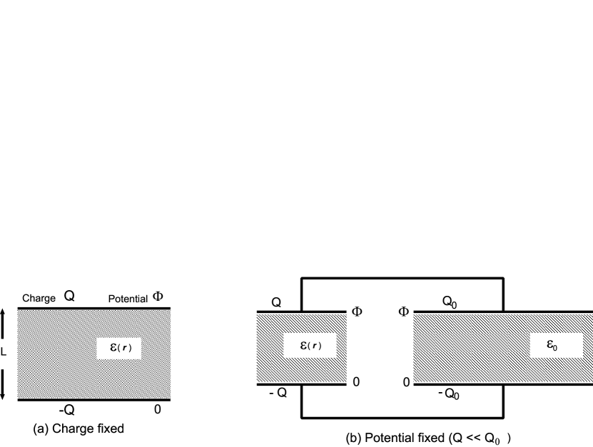
Figure 1: (a) System of a capacitor and a dielectric material with inhomogeneous dielectric constant $\varepsilon({\mbox{\boldmath$r$}})$ at fixed capacitor charge $Q$. The potential difference $\Phi$ is a fluctuating quantity dependent on $\varepsilon({\mbox{\boldmath$r$}})$. (b) Two capacitors connected in parallel with charges $Q$ and $Q_{0}$. The smaller one contains an inhomogeneous dielectric material, and the larger one a homogeneous dielectric material. In the limit $Q/Q_{0}\rightarrow 0$, the potential difference $\Phi$ becomes fixed, while $Q$ is a fluctuating quantity.

The first typical experimental geometry is shown in Fig.1a, where we insert our system between two parallel metallic plates with area $S$ and separation distance $L$. We assume $S^{1/2}\gg L$ and neglect the effects of edge fields. Generalization to other geometries is straightforward. The $z$ axis is taken perpendicularly to the plates. Let the average surface charge density of the upper plate be $\sigma_{\rm ex}$ and that of the lower plate be $-\sigma_{\rm ex}$. The total charge on the upper plate is

$$Q=S\sigma_{\rm ex}.$$ (2.1)

The Ginzburg-Landau free energy functional $F$ consists of a chemical part $F_{\rm ch}\{\psi,{\mbox{\boldmath$p$}},\rho\}$ and an electrostatic part $F_{\rm st}\{{\mbox{\boldmath$p$}},\rho,Q\}$ as

$$F=F_{\rm ch}\{\psi,{\mbox{\boldmath$p$}},\rho\}+F_{\rm st}\{{\mbox{\boldmath$p$}},\rho,Q\},$$ (2.2)

where $\psi$ represents a set of variables including the order parameter. In ferroelectric systems $p$ is the order parameter. The equilibrium distribution of the gross variables is given by const.$\exp(-F/k_{\rm B}T)$ at each fixed $Q$. We determine $F_{\rm st}$ as follows. If infinitesimal deviations $\delta{\mbox{\boldmath$p$}}$, $\delta\rho$, and $\delta Q$ are superimposed on $p$, $\rho$, and $Q$, the incremental change of $F_{\rm st}$ should be given by the work done by the electric field,

$$\delta F_{\rm st} = F_{\rm st}\{{\mbox{\boldmath$p$}}+\delta{\mbox{\boldmath$p$}},\rho+\delta\rho,Q+\delta Q\}-F_{\rm st}\{{\mbox{\boldmath$p$}},\rho,Q\}$$ (2.3)

$$= \int d{\mbox{\boldmath$r$}}[-{\mbox{\boldmath$E$}}\cdot{\delta{\mbox{\boldmath$p$}}}+\phi\delta\rho]+\Phi\delta Q,$$

where the space integral is within the system between the plates, ${\mbox{\boldmath$E$}}=-\nabla\phi$ is the electric field vector, and $\Phi$ is the potential difference between the two plates. The electric potential $\phi$ may be set equal to $0$ at the lower plate and $\Phi$ at the upper plate. The electric induction $\mbox{\boldmath$D$}={\mbox{\boldmath$E$}}+4\pi{\mbox{\boldmath$P$}}$ satisfies

$$\nabla\cdot{\mbox{\boldmath$D$}}=-\nabla^{2}\phi+4\pi\nabla\cdot{\mbox{\boldmath$p$}}=4\pi\rho,$$ (2.4)

in the bulk region. The potential $\phi$ satisfies

$$-\nabla^{2}\phi=4\pi\rho_{\rm eff},$$ (2.5)

where

$$\rho_{\rm eff}({\mbox{\boldmath$r$}})=\rho({\mbox{\boldmath$r$}})-\nabla\cdot{\mbox{\boldmath$p$}}({\mbox{\boldmath$r$}})$$ (2.6)

is the effective charge density. The boundary conditions at $z=0$ and $L$ are

$$E_{x}=E_{y}=0,\quad D_{z}=-4\pi\sigma_{\rm ex}.$$ (2.7)

With these relations of electrostatics we can integrate (2.3) formally as

$$F_{\rm st}=\frac{1}{8\pi}\int d{\mbox{\boldmath$r$}}{\mbox{\boldmath$E$}}^{2}.$$ (2.8)

In fact (2.8) leads to the second line of (2.3) if use is made of $\delta({\mbox{\boldmath$E$}}^{2})=-2{\nabla\phi}\cdot\delta{\mbox{\boldmath$D$}}-8\pi{\mbox{\boldmath$E$}}\cdot\delta{\mbox{\boldmath$p$}}=-2\nabla(\phi\delta{\mbox{\boldmath$D$}})+8\pi(\phi\delta\rho-{\mbox{\boldmath$E$}}\cdot\delta{\mbox{\boldmath$p$}})$.

To explicitly express $F_{\rm st}$ in terms of the gross variables, we first assume that all the quantities depend only on $z$ and $p$ is along the $z$ axis, for simplicity [28]. If we define $w(z)=\int_{0}^{z}dz^{\prime}\rho(z^{\prime})$, we obtain

$$\phi(z)=4\pi\int_{0}^{z}dz^{\prime}[p_{z}(z^{\prime})+\sigma_{\rm ex}-w(z^{\prime})].$$ (2.9)

From the overall charge neutrality condition we require $w(L)=0$, so (2.7) is satisfied and

$$F_{\rm st}=\frac{S}{8\pi}\int_{0}^{L}dzE_{z}(z)^{2}=2\pi S\int_{0}^{L}dz[p_{z}(z)+\sigma_{\rm ex}-w(z)]^{2}.$$ (2.10)

For general inhomogeneous $p$ and $\rho$, we define the lateral averages,

$$\bar{\mbox{\boldmath$p$}}(z)=\frac{1}{S}\int d{\mbox{\boldmath$r$}}_{\perp}{\mbox{\boldmath$p$}}({\mbox{\boldmath$r$}}),\quad{\bar{\rho}}(z)=\frac{1}{S}\int d{\mbox{\boldmath$r$}}_{\perp}\rho({\mbox{\boldmath$r$}}),$$ (2.11)

where ${\mbox{\boldmath$r$}}_{\perp}=(x,y)$ is the lateral position vector. We may assume $\bar{p}_{x}={\bar{p}}_{y}=0$ from the geometrical symmetry in the limit $S^{1/2}/L\rightarrow\infty$. The effective charge density $\rho_{\rm eff}$ is divided into the lateral average $\bar{\rho}-d{\bar{p}_{z}}/dz$ and the inhomogeneous part,

$$\rho_{\rm inh}({\mbox{\boldmath$r$}})=[\rho({\mbox{\boldmath$r$}})-{\bar{\rho}}(z)]-\nabla\cdot[{\mbox{\boldmath$p$}}({\mbox{\boldmath$r$}})-{\bar{\mbox{\boldmath$p$}}}(z)].$$ (2.12)

The electric potential is expressed as

$$\phi({\mbox{\boldmath$r$}})=4\pi\int_{0}^{z}dz^{\prime}[{\bar{p}}_{z}(z^{\prime})+\sigma_{\rm ex}-{\bar{w}}(z^{\prime})]+4\pi\int d{\mbox{\boldmath$r$}}^{\prime}G({\mbox{\boldmath$r$}},{\mbox{\boldmath$r$}}^{\prime})\rho_{\rm inh}({\mbox{\boldmath$r$}}^{\prime}).$$ (2.13)

The first term is of the same form as (2.9) and

$${\bar{w}}(z)=\int_{0}^{z}dz^{\prime}{\bar{\rho}}(z^{\prime}),$$ (2.14)

which vanishes at $z=0$ and $L$. The Green function $G({\mbox{\boldmath$r$}},{\mbox{\boldmath$r$}}^{\prime})=G({\mbox{\boldmath$r$}}^{\prime},{\mbox{\boldmath$r$}})$ satisfies

$$\nabla^{2}G({\mbox{\boldmath$r$}},{\mbox{\boldmath$r$}}^{\prime})=-\delta({\mbox{\boldmath$r$}}-{\mbox{\boldmath$r$}}^{\prime})$$ (2.15)

and vanishes as $r$ and ${\mbox{\boldmath$r$}}^{\prime}$ approach the surfaces of the conductors as

$$\lim_{z\rightarrow 0,L}G({\mbox{\boldmath$r$}},{\mbox{\boldmath$r$}}^{\prime})=\lim_{z^{\prime}\rightarrow 0,L}G({\mbox{\boldmath$r$}},{\mbox{\boldmath$r$}}^{\prime})=0.$$ (2.16)

Then we have $E_{x}=E_{y}=$ at $z=0$ and $L$. The potential difference $\Phi$ is written as

$$\Phi = 4\pi\int_{0}^{L}dz[{\bar{p}}_{z}(z)+\sigma_{\rm ex}-{\bar{w}}(z)]$$ (2.17)

$$= 4\pi L\langle{p_{z}+\sigma_{\rm ex}+z\rho}\rangle_{\rm s},$$

where $\langle{\cdots}\rangle_{\rm s}=\int d{\mbox{\boldmath$r$}}(\cdots)/SL$ represents the space average and use has been made of $\langle{\rho}\rangle_{\rm s}=0$. This relation may also be written as

$$\Phi/4\pi L-\langle{p_{z}}\rangle_{\rm s}=Q/S-\langle{(L/2-z)\rho}\rangle_{\rm s},$$ (2.18)

which relates the mean electric field $-\Phi/L$ and the capacitor charge $Q$. The second term on the right hand side becomes important when the charge is accumulated near the capacitor plates in electric field.

Because we are taking the limit $S^{1/2}/L\rightarrow\infty$, the translational invariance $G({\mbox{\boldmath$r$}},{\mbox{\boldmath$r$}}^{\prime})=G({\mbox{\boldmath$r$}}_{\perp}-{\mbox{\boldmath$r$}}_{\perp}^{\prime},z,z^{\prime})$ holds in the $xy$ plane. The Fourier transformation $G_{k}(z,z^{\prime})$ in the $xy$ plane satisfies $(-\nabla_{z}^{2}+k^{2})G_{k}(z,z^{\prime})=\delta(z-z^{\prime})$ and becomes [8]

$$G_{k}(z,z^{\prime}) = G_{k}(z^{\prime},z)=\frac{1}{2k}e^{-k|z-z^{\prime}|}-\frac{1}{2k\sinh(kL)}$$ (2.19)

$$\times\bigg{[}\sinh(kz)e^{-k(L-z^{\prime})}+\sinh(kL-kz)e^{-kz^{\prime}}\bigg{]}.$$

In particular, in the long wavelength limit $k\rightarrow 0$, we have

$$G_{0}(z,z^{\prime})=\lim_{k\rightarrow 0}G_{k}(z,z^{\prime})=\frac{1}{2}[z+z^{\prime}-|z-z^{\prime}|]-zz^{\prime}/L.$$ (2.20)

From (2.17) and (2.20), as it should be the case, the potential $\phi$ is also expressed as

$$\phi({\mbox{\boldmath$r$}})=\Phi z/L+4\pi\int d{\mbox{\boldmath$r$}}^{\prime}G({\mbox{\boldmath$r$}},{\mbox{\boldmath$r$}}^{\prime})\rho_{\rm eff}({\mbox{\boldmath$r$}}^{\prime}).$$ (2.21)

The electrostatic energy is written in terms of $\rho_{\rm inh}$ as

$$F_{\rm st}=2\pi S\int_{0}^{L}dz\bigg{[}{\bar{p}}_{z}(z)+\sigma_{\rm ex}-w(z)\bigg{]}^{2}+2\pi\int d{\mbox{\boldmath$r$}}\int d{\mbox{\boldmath$r$}}^{\prime}\rho_{\rm inh}({\mbox{\boldmath$r$}})G({\mbox{\boldmath$r$}},{\mbox{\boldmath$r$}}^{\prime})\rho_{\rm inh}({\mbox{\boldmath$r$}}^{\prime}).$$ (2.22)

With the aid of (2.17) and (2.20), $F_{\rm st}$ in terms of $\rho_{\rm eff}$ reads

$$F_{\rm st}=\frac{S}{8\pi L}\Phi^{2}+2\pi\int d{\mbox{\boldmath$r$}}\int d{\mbox{\boldmath$r$}}^{\prime}\rho_{\rm eff}({\mbox{\boldmath$r$}})G({\mbox{\boldmath$r$}},{\mbox{\boldmath$r$}}^{\prime})\rho_{\rm eff}({\mbox{\boldmath$r$}}^{\prime}).$$ (2.23)

2.2 Dielectrics under given capacitor potential

In the previous case, the capacitor charge $Q$ is a control parameter and the potential difference $\Phi$ is a fluctuating quantity. We may also control $\Phi$ by using (i) a battery at a fixed potential difference connected to the capacitor or (ii) another large capacitor connected in parallel to the capacitor containing a dielectric material as in Fig.1b. We examine the well-defined case (ii). The area $S_{0}$ and the charge $Q_{0}$ of the large capacitor are much larger than $S$ and $Q$, respectively, so the large capacitor acts as a charge reservoir. We are supposing an experiment in which the total charge $Q_{\rm tot}=Q_{0}+Q$ is fixed and the potential difference is commonly given by $\Phi=Q_{0}/C_{0}$, where $C_{0}$ is the capacitance of the large capacitor. Obviously, in the limit $Q/Q_{0}\sim S/S_{0}\rightarrow 0$, the deviation of $\Phi$ from the upper bound $\Phi_{\rm tot}=Q_{\rm tot}/C_{0}$ becomes negligible. Because the electrostatic energy of the large capacitor is given by $E_{0}=Q_{0}^{2}/2C_{0}=(Q_{\rm tot}^{2}/2C_{0})(1-Q/Q_{\rm tot})^{2}$, we obtain

$$E_{0}\cong(Q_{\rm tot}^{2}/2C_{0})-\Phi Q,$$ (2.24)

where the first term is constant and a term of order $(Q/Q_{\rm tot})^{2}$ is neglected. Therefore, for the total system including the two capacitors, the potential difference $\Phi$ is a control parameter and the appropriate free energy functional is given by the Legendre transformation [1],

$$G=F-\Phi Q.$$ (2.25)

If $\Phi$ is fixed, $Q$ is a fluctuating quantity determined by (2.18). The equilibrium distribution of the gross variables is given by const.$\exp(-G/k_{\rm B}T)$ at each fixed $\Phi$.

2.3 Dielectrics in vacuum and dipolar ferromagnets

There is another typical case, in which a sample of dielectrics is placed in vacuum. There is no polarization and charge immediately outside the sample, but there can be an applied electric field created by capacitor plates far from the sample. As far as I am aware, simulations of phase transitions in dipolar particle systems have been performed under this boundary condition [29], where the particles are assumed to interact via the dipolar potential $\propto\delta_{ij}/r^{3}-3x_{i}x_{j}/r^{5}$ even close to the surface. In ferromagnetic systems there is no magnetic charge and this boundary condition is always assumed [30].

We assume no free charge ($\rho=0$) and apply an electric field $E_{\rm ex}$ along the $z$ axis. The electrostatic potential is given by

$$\phi({\mbox{\boldmath$r$}}) = -E_{\rm ex}z+\int d{\mbox{\boldmath$r$}}^{\prime}G_{0}({\mbox{\boldmath$r$}},{\mbox{\boldmath$r$}}^{\prime})\rho_{\rm eff}({\mbox{\boldmath$r$}}^{\prime})+\int daG_{0}({\mbox{\boldmath$r$}},{\mbox{\boldmath$r$}}_{a})\sigma_{\rm eff}({\mbox{\boldmath$r$}}_{a})$$ (2.26)

$$= -E_{\rm ex}z+\int d{\mbox{\boldmath$r$}}^{\prime}{\mbox{\boldmath$p$}}({\mbox{\boldmath$r$}}^{\prime})\cdot\nabla^{\prime}G_{0}({\mbox{\boldmath$r$}}-{\mbox{\boldmath$r$}}^{\prime}).$$

In the first line $\rho_{\rm eff}=-\nabla\cdot{\mbox{\boldmath$p$}}$ is the effective charge as given in (2.6), $\sigma_{\rm eff}={\mbox{\boldmath$p$}}\cdot{\mbox{\boldmath$n$}}$ is the effective surface charge with $n$ being the outward normal unit vector at the surface, and ${\mbox{\boldmath$r$}}_{a}$ represents the surface point. In the second line the space integral is within the sample and $\nabla^{\prime}=\partial/\partial{\mbox{\boldmath$r$}}^{\prime}$. Since there is no capacitor charge in contact with the system, $G_{0}$ is of the usual Coulombic form,

$$G_{0}({\mbox{\boldmath$r$}}-{\mbox{\boldmath$r$}}^{\prime})={1}/{|{\mbox{\boldmath$r$}}-{\mbox{\boldmath$r$}}^{\prime}|}.$$ (2.27)

The total free energy consists of the chemical part and electrostatic part as $F=F_{\rm ch}\{\psi,{\mbox{\boldmath$p$}}\}+F_{\rm st}\{{\mbox{\boldmath$p$}}\}$. The latter is the usual dipolar interaction,

$$F_{\rm st}=-\int d{\mbox{\boldmath$r$}}E_{\rm ex}p_{z}+\frac{1}{2}\int d{\mbox{\boldmath$r$}}\int d{\mbox{\boldmath$r$}}^{\prime}\sum_{ij}p_{i}({\mbox{\boldmath$r$}})p_{j}({\mbox{\boldmath$r$}}^{\prime})[-\nabla_{i}\nabla_{j}G_{0}({\mbox{\boldmath$r$}}-{\mbox{\boldmath$r$}}^{\prime})],$$ (2.28)

which satisfies $\delta F_{\rm st}/\delta{\mbox{\boldmath$p$}}=-{\mbox{\boldmath$E$}}$ in (2.3). Here $-\nabla_{i}\nabla_{j}G_{0}({\mbox{\boldmath$r$}})=\delta_{ij}/r^{3}-3x_{i}x_{j}/r^{5}$, as ought to be the case. In the ferromagnetic case, $p$ and ${E}_{\rm ex}$ correspond to the magnetization and the applied magnetic field, respectively [1].

The above electrostatic (magnetic) energy (2.28) depends on the sample shape due to the depolarization (demagnetization) effect, so the phase transition to a ferroelectric (ferromagnetic) phase becomes shape-dependent [29]. As is well known, if the dielectric constant $\varepsilon$ is uniform in the sample, the field inside is given by $E_{\rm ex}/\varepsilon$ for a thin plate and $3E_{\rm ex}/(2+\varepsilon)$ for a sphere along the $z$ axis.

3 Near-critical fluids without ions

As an application of the general scheme in Section 2, we consider a near-critical fluid in the geometry of Fig.1a. We will use the results already presented in Section 1.

3.1 General relations in the charge-free case

In the absence of free charges ($\rho=0$), $F_{\rm ch}$ in (2.2) is written as

$$F_{\rm ch}\{\psi,{\mbox{\boldmath$p$}}\}=F_{0}\{\psi\}+\int d{\mbox{\boldmath$r$}}\frac{1}{2\chi}{\mbox{\boldmath$p$}}^{2},$$ (3.1)

where $\chi$ represents the electric susceptibility. The first term is the usual free energy functional for the order parameter $\psi$. Close to the critical point it is of the form,

$$F_{0}\{\psi\}=k_{\rm B}T_{\rm c}\int d{\mbox{\boldmath$r$}}\bigg{[}\frac{a_{0}}{2}\tau\psi^{2}+\frac{u_{0}}{4}\psi^{4}+\frac{K_{0}}{2}|\nabla\psi|^{2}\bigg{]},$$ (3.2)

where $a_{0}$, $u_{0}$ and $K_{0}$ are positive constants, and $\tau$ is the reduced temperature. The term $\propto\int d{\mbox{\boldmath$r$}}\psi$ is not written (because $\psi$ is a conserved variable). Use of (2.3) gives

$$\delta F=\delta F_{0}+\int d{\mbox{\boldmath$r$}}\bigg{[}(\chi^{-1}{\mbox{\boldmath$p$}}-{\mbox{\boldmath$E$}})\cdot{\delta{\mbox{\boldmath$p$}}}-\frac{1}{2\chi^{2}}{\mbox{\boldmath$p$}}^{2}\delta\chi\bigg{]}+\Phi\delta Q.$$ (3.3)

Thus $F$ is minimized for

$${\mbox{\boldmath$p$}}=\chi{\mbox{\boldmath$E$}},\quad{\mbox{\boldmath$D$}}=\varepsilon{\mbox{\boldmath$E$}}.$$ (3.4)

The static dielectric constant is

$$\varepsilon=1+4\pi\chi$$ (3.5)

and depends locally on the order parameter $\psi$ as in (1.2). In usual fluids $p$ rapidly relaxes to $\chi{\mbox{\boldmath$E$}}$ on a microscopic time scale, so (3.4) may be assumed even in nonequilibrium. Then $p$ is determined by $\psi$ and $Q$. The charge-free condition within the fluid $\nabla\cdot{\mbox{\boldmath$D$}}=0$ is written as

$$\nabla\cdot(\varepsilon\nabla\phi)=0.$$ (3.6)

From the general expressions (2.8) and (3.1) with the aid of (3.4) we obtain

$$F=F_{0}\{\psi\}+\frac{1}{8\pi}\int d{\mbox{\boldmath$r$}}{\mbox{\boldmath$E$}}\cdot{\mbox{\boldmath$D$}}=F_{0}\{\psi\}+\frac{1}{2}\Phi Q.$$ (3.7)

The expression in terms of $Q$ also follows directly from integration of $\delta F=\Phi\delta Q$ at fixed $\psi$, where the factor $1/2$ arises because the ratio $\Phi/Q$ is a functional of $\psi$ only and is independent of $Q$ from (3.4). On the other hand, in the fixed-potential case in the geometry of Fig.1b, the free energy functional $G$ in (2.25) is written as

$$G=F_{0}\{\psi\}-\frac{1}{8\pi}\int d{\mbox{\boldmath$r$}}{\mbox{\boldmath$E$}}\cdot{\mbox{\boldmath$D$}}=F_{0}\{\psi\}-\frac{1}{2}\Phi Q.$$ (3.8)

The electrostatic parts $\Delta F=F-F_{0}$ and $\Delta G=G-F_{0}$ are functionals of $\varepsilon({\mbox{\boldmath$r$}})$ at fixed $Q$ and $\Phi$, respectively. The functional derivative of $\Delta F$ at fixed $Q$ and that of $\Delta G$ at fixed $\Phi$ with respect to $\varepsilon$ are both of the same form,

$$\bigg{(}\frac{\delta}{\delta\varepsilon}{\Delta F}\bigg{)}_{Q}=\bigg{(}\frac{\delta}{\delta\varepsilon}{\Delta G}\bigg{)}_{\Phi}=-\frac{1}{8\pi}{|\mbox{\boldmath$E$}|}^{2},$$ (3.9)

because $\int d{\mbox{\boldmath$r$}}{\mbox{\boldmath$E$}}\cdot\delta{\mbox{\boldmath$D$}}=-\int d{\mbox{\boldmath$r$}}\nabla{\phi}\cdot\delta{\mbox{\boldmath$D$}}=0$ at fixed $Q$ and $\int d{\mbox{\boldmath$r$}}{\mbox{\boldmath$D$}}\cdot\delta{\mbox{\boldmath$E$}}=0$ at fixed $\Phi$. These relations directly follow from (3.3) under ${\mbox{\boldmath$p$}}=\chi{\mbox{\boldmath$E$}}$. Even if a sample is placed in vacuum, $(\delta\Delta F/\delta\varepsilon)_{E_{0}}$ assumes the same form. To derive (3.9) more evidently, we may assume that $\varepsilon=\varepsilon(z)$ is a function of $z$ only. Then we explicitly obtain $\Delta F=2\pi Q^{2}\int_{0}^{L}dz\varepsilon(z)^{-1}$ and $\Delta G=-(8\pi)^{-1}S\Phi^{2}/\int_{0}^{L}dz\varepsilon(z)^{-1}$ to confirm (3.9).

3.2 Landau expansion and critical behavior

We assume that a constant electric field ${\mbox{\boldmath$E$}}_{0}=(0,0,-E_{0})$ is applied in the negative $z$ direction. Then $\varepsilon_{2}E_{0}^{2}/4\pi k_{\rm B}T_{\rm c}(=A_{0}\tau_{\rm c}$ in (3.19)) and $(\varepsilon_{1}^{2}/\varepsilon_{0})E_{0}^{2}/4\pi k_{\rm B}T_{\rm c}(=g_{\rm e}$ in (3.16)) are two relevant parameters representing the influence of electric field. We assume that they are independent of the upper cut-off $\Lambda$ of the coarse-graining, while the coefficients in $F_{0}$ in (3.2) depend on $\Lambda$ [22]. This causes some delicate issues. Theory should be made such that the observable quantities are independent of $\Lambda$.

We expand the electrostatic free energy with respect to the order parameter $\psi$. In the following we assume the fixed charge condition, but the same expressions follow in the fixed potential condition owing to (3.9). Let the electric field be written as ${\mbox{\boldmath$E$}}={\mbox{\boldmath$E$}}_{0}-\nabla\delta\phi$, where $\delta\phi$ is the deviation of the electric potential induced by $\delta\varepsilon=\varepsilon-\langle{\varepsilon}\rangle$. Then (3.9) is expanded as

$$\bigg{(}\frac{\delta}{\delta\varepsilon}{\Delta F}\bigg{)}_{Q}=-\frac{1}{8\pi}E_{0}^{2}+\frac{1}{4\pi}{\mbox{\boldmath$E$}}_{0}\cdot\nabla\delta\phi+\cdots.$$ (3.10)

To first order in $\delta\varepsilon$ the charge-free condition (3.6) becomes ${\langle{\varepsilon}\rangle}\nabla^{2}\delta\phi={\mbox{\boldmath$E$}}_{0}\cdot\nabla\delta\varepsilon$. Using the Green function $G({\mbox{\boldmath$r$}},{\mbox{\boldmath$r$}}^{\prime})$ in (2.15) and $\langle{\varepsilon}\rangle\cong\varepsilon_{0}$, we obtain

$$\delta\phi({\mbox{\boldmath$r$}})=-\frac{1}{4\pi\varepsilon_{0}}\int d{\mbox{\boldmath$r$}}^{\prime}G({\mbox{\boldmath$r$}},{\mbox{\boldmath$r$}}^{\prime}){\mbox{\boldmath$E$}}_{0}\cdot\nabla^{\prime}\delta\varepsilon({\mbox{\boldmath$r$}}^{\prime}).$$ (3.11)

The electrostatic free energy ${\Delta F}=F-{F}_{0}$ is composed of two parts up to order $O(\delta\varepsilon^{2})$. The first part is

$${F}_{e0}=-\frac{1}{8\pi}\int d{\mbox{\boldmath$r$}}{E}_{0}^{2}{\varepsilon}=-\frac{1}{8\pi}\int d{\mbox{\boldmath$r$}}{E}_{0}^{2}\bigg{(}{\varepsilon}_{0}+\varepsilon_{1}\psi+\frac{1}{2}\varepsilon_{2}\psi^{2}\bigg{)}.$$ (3.12)

The linear term $(\propto\int d{\mbox{\boldmath$r$}}\psi)$ is irrelevant for fluids and the bilinear term $(\propto\int d{\mbox{\boldmath$r$}}\psi^{2})$ gives rise to a shift of the critical temperature as will be shown in (3.19) and (3.22). The second part is a dipolar interaction arising from the second term in (3.10),

$${F}_{\rm dip}=\frac{1}{8\pi}A_{\rm s}E_{0}^{2}\int d{\mbox{\boldmath$r$}}\int d{\mbox{\boldmath$r$}}^{\prime}[\nabla_{z}\psi({\mbox{\boldmath$r$}})]G({\mbox{\boldmath$r$}},{\mbox{\boldmath$r$}}^{\prime})[\nabla_{z}\psi({\mbox{\boldmath$r$}}^{\prime})],$$ (3.13)

where $\nabla_{z}=\partial/\partial z$. The coefficient $A_{\rm s}$ is defined by

$$A_{\rm s}=\varepsilon_{1}^{2}/{\bar{\varepsilon}}\cong\varepsilon_{1}^{2}/{\varepsilon_{0}}.$$ (3.14)

which is small for pure fluids ($=(\varepsilon_{0}-1)^{2}(\varepsilon_{0}+2)^{2}/9\varepsilon_{0}$ from Clausius-Mossotti), but can be $10-100$ for polar binary mixtures. The $F_{\rm dip}$ is positive-definite for the fluctuations varying along ${\mbox{\boldmath$E$}}_{0}$ but vanishes for those varying perpendicularly to ${\mbox{\boldmath$E$}}_{0}$. Thus $F_{\rm dip}$ produces no shift of $T_{\rm c}$ in the mean-field theory, but its suppresses the fluctuations leading to a fluctuation contribution to the shift as in (3.23) below.

Far from the capacitor plates we may set $G({\mbox{\boldmath$r$}},{\mbox{\boldmath$r$}}^{\prime})=1/4\pi|{\mbox{\boldmath$r$}}-{\mbox{\boldmath$r$}}^{\prime}|$. Picking up only the Fourier components $\psi_{\small{\mbox{\boldmath$q$}}}=\int d{\mbox{\boldmath$r$}}\psi({\mbox{\boldmath$r$}}){\rm e}^{i\small{\mbox{\boldmath$q$}}\cdot\small{\mbox{\boldmath$r$}}}$ with $qL\gg 1$, we obtain

$${F}_{\rm dip}={\frac{1}{2}}k_{\rm B}T_{\rm c}g_{\rm e}\int_{\mbox{\boldmath$q$}}\hat{q}_{z}^{2}|\psi_{\small{\mbox{\boldmath$q$}}}|^{2},$$ (3.15)

where $\hat{q}_{z}=q_{z}/q$. The strength of the interaction is given by

$$g_{\rm e}=(4\pi k_{\rm B}T_{\rm c})^{-1}A_{\rm s}{E_{0}}^{2}.$$ (3.16)

A similar dipolar interaction is well-known for uniaxial ferromagnets [30, 33]. At the critical density (or composition) in one-phase states, the structure factor $I({\mbox{\boldmath$q$}})$ in the presence of ${F}_{\rm dip}$ becomes uniaxial as

$$I({\mbox{\boldmath$q$}})=[a_{0}(\tau-\tau_{\rm c})+g_{\rm e}\hat{q}_{z}^{2}+K_{0}q^{2}]^{-1},$$ (3.17)

where $\tau_{\rm c}$ is a shift induced by electric field. For $g_{\rm e}\hat{q}_{z}^{2}>a_{0}\tau_{\rm c}$, the intensity decreases with increasing electric field even if $\tau_{\rm c}>0$.

(i) Weak field regime: If $g_{{\rm e}}$ is smaller than $a_{0}\tau={\hat{\chi}}^{-1}$, the electric field is weak and the structure factor may be expanded as

$$I({\mbox{\boldmath$q$}})=I_{0}(q)+I_{0}(q)^{2}(a_{0}\tau_{\rm c}-g_{\rm e}\hat{q}_{z}^{2})+\cdots,$$ (3.18)

where $I_{0}(q)={\hat{\chi}}/(1+q^{2}\xi^{2})$ is the intensity at zero electric field with ${\hat{\chi}}=I(0)$. The apparent shift arises from the bilinear term ($\propto\psi^{2}$) in $F_{e0}$ in (3.12):

$$a_{0}\tau_{\rm c}={\varepsilon_{2}}{E}_{0}^{2}/4\pi k_{\rm B}T_{\rm c}={\varepsilon_{2}}{g_{\rm e}}/A_{\rm s}.$$ (3.19)

Note that $a_{0}\tau_{\rm c}$ and hence (3.18) are independent of $\Lambda$. The usual critical behavior at long wavelengths $q\xi<1$ follows for $\Lambda\xi\sim 1$, where $\xi=\xi_{+0}\tau^{-\nu}$ is the correlation length. The asymptotic scaling relations are ${\hat{\chi}}=\Gamma\tau^{-\gamma}$ (or $a_{0}=\Gamma^{-1}\tau^{\gamma-1}$) and $K_{0}={\hat{\chi}}^{-1}\xi^{2}=\Gamma^{-1}\xi_{+0}^{2}\tau^{-\nu\eta}$, where $\Gamma$ is a constant, and $\gamma\cong 1.24$, $\nu\cong 0.625$, and $\eta=0.03-0.05$ are the usual critical exponents.

(ii) Strong field regime: The electric field is strong for $\tau-\tau_{\rm c}<\tau_{{\rm e}}$. The crossover reduced temperature $\tau_{{\rm e}}$ and the characteristic wave number $k_{{\rm e}}$ are written as

$$\tau_{{\rm e}}=(\Gamma g_{{\rm e}})^{1/\gamma},\quad k_{{\rm e}}=\xi_{+0}^{-1}(\Gamma g_{{\rm e}})^{\nu/\gamma}.$$ (3.20)

As a rough estimate, we set $\Gamma\sim\xi_{+0}^{3}$, $\xi_{+0}\sim 2.5\times 10^{-8}$cm, and $T_{\rm c}\sim 300$K to obtain $\tau_{\rm e}\sim 10^{-6}A_{\rm s}^{0.8}E_{0}^{1.6}$ with $E_{0}$ in units of $10^{4}$V$/$cm. There is no experimental report in this regime. According to the renormalization group theory in the presence of the uniaxial dipolar interaction (3.15) (which treats $F_{0}+F_{\rm dip})$[33], there is no renormalization of the coefficient $g_{\rm e}$ and the dipolar interaction strongly suppresses the fluctuations with wave numbers smaller than $k_{\rm e}$ in the temperature range $\tau-\tau_{\rm c}<\tau_{{\rm e}}$ resulting in mean field critical behavior for $d\geq d_{\rm c}=3$. For these fluctuations we may set $\Lambda\sim k_{{\rm e}}$ to obtain the renormalized coefficients,

$$a_{0}=\Gamma^{-1}\tau_{{\rm e}}^{\gamma-1},\quad K_{0}=\Gamma^{-1}\xi_{+0}^{2}\tau_{{\rm e}}^{-\nu\eta},\quad u_{0}=g^{*}K_{0}^{2}k_{{\rm e}}^{\epsilon}/K_{d},$$ (3.21)

where $K_{d}=(2\pi)^{-d}2\pi^{d/2}/\Gamma(d/2)$, $\epsilon=4-d$, and $g^{*}=\epsilon/9+O(\epsilon^{2})$ is the fixed point value of the coupling constant $g=K_{d}u_{0}/K_{0}^{2}\Lambda^{\epsilon}$ [22]. The shift $\tau_{\rm c}$ in (3.17) in strong field consists of two terms as $\tau_{\rm c}=\tau_{{\rm c}1}+\tau_{{\rm c}2}$. The origin of $\tau_{{\rm c}1}$ is the same as that of $\tau_{{\rm c}}$ in (3.19). Here using (3.20) and (3.21) we obtain

$$\tau_{{\rm c}1}={\varepsilon_{2}}E_{0}^{2}/4\pi a_{0}k_{\rm B}T=(\varepsilon_{2}/A_{\rm s})\tau_{{\rm e}}.$$ (3.22)

The $\tau_{{\rm c}2}$ arises from the quartic term ($\propto u_{0}$) in $F_{0}$ in (3.2):

$$\tau_{{\rm c}2}=-\frac{3}{a_{0}}u_{0}\int_{\mbox{\boldmath$q$}}\bigg{[}\frac{1}{g_{{\rm e}}\hat{q}_{z}^{2}+K_{0}q^{2}}-\frac{1}{K_{0}q^{2}}\bigg{]}=3g^{*}C_{d}\tau_{{\rm e}},$$ (3.23)

where $C_{d}=K_{d}^{-1}\int_{\mbox{\boldmath$\ell$}}\ell_{z}^{2}/\ell^{2}(\ell^{4}+\ell_{z}^{2})$ ($=\pi/4$ at $d=3$). The $\tau_{{\rm c}2}$ is a positive fluctuation contribution meaningful only in strong field. (A similar shift was calculated for near-critical fluids in shear flow [22].) Therefore both $\tau_{{\rm c}1}$ and $\tau_{{\rm c}2}$ are of order $\tau_{{\rm e}}$. We also consider the correlation function $g({\mbox{\boldmath$r$}})=\int_{\mbox{\boldmath$q$}}I({\mbox{\boldmath$q$}})\rm{e}^{i{\small{\mbox{\boldmath$q$}}}\cdot{\small{\mbox{\boldmath$r$}}}}$ in strong field. From (3.17) and (3.21) the scaling form $g({\mbox{\boldmath$r$}})=G(x/\xi_{\perp},y/\xi_{\perp},z/\xi_{\parallel})/K_{0}\xi_{\parallel}$ holds with

$$\xi_{\perp}=k_{\rm e}^{-1}[\tau_{\rm e}/(\tau-\tau_{\rm c})]^{1/2},\quad\xi_{\parallel}=k_{\rm e}\xi_{\perp}^{2}=k_{\rm e}^{-1}\tau_{\rm e}/(\tau-\tau_{\rm c})>\xi_{\perp}.$$ (3.24)

Here $G(0,0,Z)\sim Z^{-3}$ for $Z\gg 1$. The large-scale critical fluctuations ($\gg k_{\rm e}^{-1}$) are elongated along the $z$ axis, as expected in experimental papers $[13]$.

We now comment on previous work.
(i) If $a_{0}$ is treated as a constant, $T_{\rm c}\tau_{{\rm c}1}$ is the mean field shift in Landau-Lifshitz’s book for pure fluids [1]. The same shift was later proposed for binary mixtures [7].
(ii) Debye and Kleboth [2] derived a reverse shift ($\Delta T_{\rm c}=-T_{\rm c}\tau_{{\rm c}1}$) neglecting the inhomogeneity of $E$ and setting ${\mbox{\boldmath$E$}}={\mbox{\boldmath$E$}}_{0}$ in (3.7). The dipolar interaction was nonexistent, leading to the normalized turbidity change ${\cal T}(E_{0})/{\cal T}(0)-1\cong\hat{\chi}a_{0}\tau_{\rm c}$ for $k\xi\ll 1$, where ${\cal T}(E_{0})$ is the turbidity in electric field (see (1.7)). They found turbidity decreases in nitrobenzene+ 2,2,4-trimethylpentane to obtain $\tau_{\rm c}=-0.5\times 10^{-4}$ at $E_{0}=45$kV$/$cm in agreement with their theory, where Hildebrand’s theory gave $a_{0}=(4.3{\rm\AA})^{-3}$ and data of $\varepsilon(\phi)$ as a function of the volume fraction $\phi$ of nitrobenzene gave $\partial^{2}\varepsilon/\partial\phi^{2}=28.7$. (Notice that their $|\tau_{\rm c}|$ is of order $\tau_{\rm e}$ in (3.20) if $A_{\rm s}\sim 10$.) Subsequent light scattering experiments detected similar suppression in a near-critical binary mixture [31] and in a polymer solution [32]. In our theory (3.18) and (3.19) hold in weak field, so for $k\xi\ll 1$ we have

$${\cal T}(E_{0})/{\cal T}(0)-1\cong\hat{\chi}(a_{0}\tau_{\rm c}-g_{\rm e}/5)\quad{\rm or}\quad\hat{\chi}(a_{0}\tau_{\rm c}-2g_{\rm e}/5)$$ (3.25)

for the polarization along the $z$ or $y$ axis. Thus we predict that the turbidity decreases for $g_{\rm e}/5>a_{0}\tau_{\rm c}$ or for $A_{\rm s}>5\varepsilon_{2}$ for any polarization. Here we expect that $A_{\rm s}$ is considerably larger than $|\varepsilon_{2}|$ in polar mixtures (see the end of Subsection 3.3 also). Complex effects also arise from a small amount of ions which are present in most binary mixtures (see Section 4).

3.3 Macroscopic dielectric constant

@

We calculate the macroscopic dielectric constant $\varepsilon_{\rm eff}=4\pi\langle{Q}\rangle/SE_{0}=\langle{D_{z}}\rangle/E_{0}$ in the absence of charges. From the charge-free condition $\nabla\cdot\langle{\mbox{\boldmath$D$}}\rangle=\nabla_{z}\langle{D_{z}}\rangle=0$, $\langle{D_{z}}\rangle$ is homogeneous in the fluid as

$$\langle{D_{z}}\rangle=\langle{\varepsilon}\rangle E_{0}-\langle{\delta\varepsilon\nabla_{z}\delta\phi}\rangle={\rm const.}$$ (3.26)

Far from the boundary surfaces, by setting $M=\langle{\psi}\rangle$, we obtain

$$\varepsilon_{\rm eff}=\varepsilon_{0}+\varepsilon_{1}M+\frac{1}{2}\varepsilon_{2}M^{2}+\int_{\mbox{\boldmath$q$}}\bigg{[}\frac{1}{2}\varepsilon_{2}-A_{\rm s}{\hat{q}_{z}^{2}}\bigg{]}I({\mbox{\boldmath$q$}}),$$ (3.27)

where the last term is the $zz$ component of the tensor in (1.3).

(i) Linear response: The linear dielectric constant $\varepsilon_{\rm eff}(0)$ is defined in the limit $E_{0}\rightarrow 0$, where $\hat{q}_{z}^{2}$ in (3.27) may be replaced by $1/3$. Because $a_{0}\psi^{2}$ corresponds to the energy density in the corresponding Ising model (see the sentences below (1.2)), the renormalization group theory gives $\langle{a_{0}\psi^{2}}\rangle={\rm const}.-A\tau^{1-\alpha}/(1-\alpha)+\cdots$ with $\alpha\cong 0.11$ (the specific-heat critical exponent) and $A=R_{\xi}^{d}/(\alpha\xi_{+0}^{d})$ at the critical density or composition above $T_{\rm c}$ [22]. In terms of this $A$, the specific heat $C_{V}$ for pure fluids and $C_{pc}$ for binary mixtures per unit volume grow as $-k_{\rm B}\partial\langle{a_{0}\psi^{2}}\rangle/\partial\tau\cong k_{\rm B}A\tau^{-\alpha}$. The $R_{\xi}^{d}=\alpha A\xi_{+0}^{d}(\cong K_{d}/4)$ is a universal number (the two-scale-factor universality). It follows that $\varepsilon_{\rm eff}(0)$ should exhibit weakly singular behavior $[4$-$6,8]$,

$$\varepsilon_{\rm eff}(0)=\varepsilon_{\rm c}+D_{1}\tau^{1-\alpha}+D_{2}\tau+\cdots.$$ (3.28)

In our theory $D_{1}=(A_{\rm s}-3\varepsilon_{2}/2)A/3a_{0}$ depends on the arbitrary cut-off $\Lambda$ since $a_{0}\propto\Lambda^{(\gamma-1)/\nu}$ for $\Lambda\gg\xi^{-1}$, indicating inadequacy of our theory at short wavelengths. To calculate $D_{1}$ correctly we need to interpolate the renormalization group theory to a microscopic theory [34]. On the other hand, the refractive index $n(\omega)=\varepsilon(\omega)^{1/2}$ at optical frequency has also been predicted to be of the form of (3.28) [4, 6]. However, despite a number of experiments, unambiguous detection of the weak singularity in these quantities has been difficult for both pure fluids and binary mixtures [10].

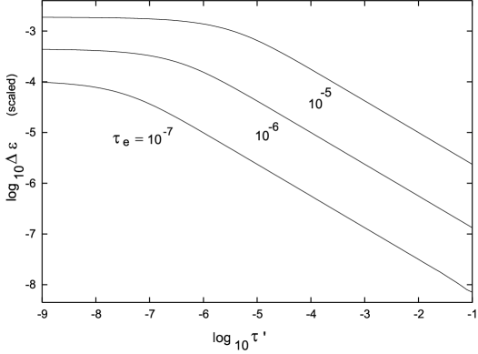
Figure 2: Nonlinear dielectric constant $\Delta\varepsilon_{\rm eff}(\tau,E_{0})$ (divided by a constant $B_{0}$) vs reduced temperature $\tau^{\prime}=\tau-\tau_{\rm c}>0$ in applied electric field $E_{0}$ for $\tau_{\rm e}=10^{-5},10^{-6},$ and $10^{-7}$, where $\tau_{\rm e}\propto E_{0}^{1.6}$ from (3.20).

(i) Nonlinear response: The nonlinear dielectric constant $\Delta\varepsilon_{\rm eff}=\varepsilon_{\rm eff}(E_{0})-\varepsilon_{\rm eff}(0)$ has been observed to become positive and grow near the critical point in polar binary mixtures $[12$-$15]$. Because small-scale fluctuations are insensitive to electric field, such critical anomaly arises from nonlinear effects at long wavelengths ($q<\kern-12.0pt\lower 5.0pt\hbox{$\displaystyle{\sim}$}\xi^{-1}$ for weak field and $q<\kern-12.0pt\lower 5.0pt\hbox{$\displaystyle{\sim}$}k_{\rm e}$ for strong field). Its calculation is therefore much easier than that of $\varepsilon_{\rm eff}(0)$. Use of the structure factor (3.17) yields

$$\Delta\varepsilon_{\rm eff} \cong \frac{1}{16\pi}(2A_{\rm s}/5-\varepsilon_{2}+\varepsilon_{2}^{2}/A_{\rm s})K_{0}^{-2}g_{{\rm e}}\xi\quad(\tau\gg\tau_{{\rm e}})$$ (3.29)

$$\cong \frac{1}{16\pi}(A_{\rm s}-\varepsilon_{2})K_{0}^{-1}k_{{\rm e}}\hskip 65.44142pt(0<\tau^{\prime}<\kern-12.0pt\lower 5.0pt\hbox{$\displaystyle{\sim}$}\tau_{{\rm e}}),$$ (3.30)

In the first line we have $K_{0}\propto\xi^{\eta}$ and $\Delta\varepsilon_{\rm eff}\propto E_{0}^{2}\xi^{1-2\eta}$, while in the second line $K_{0}\propto k_{\rm e}^{-\eta}$ and $\Delta\varepsilon_{\rm eff}\propto E_{0}^{(1+\eta)/(2-\eta)}$. Here we set $\tau^{\prime}=\tau-\tau_{{\rm c}}>0$. Then $\tau^{\prime}\cong\tau$ for weak field. If $\Delta\varepsilon_{\rm eff}$ is positive for any $\tau^{\prime}$, we need to require $A_{\rm s}>\varepsilon_{2}$. Previously we calculated (3.29) without the terms involving $\varepsilon_{2}$ [8]. For general $\tau^{\prime}/\tau_{\rm e}$ we find the scaling,

$$\Delta\varepsilon_{\rm eff}=B_{0}\tau_{\rm e}^{\nu(1+\eta)}{F}_{\rm non}(k_{\rm e}\xi),$$ (3.31)

where $B_{0}$ is a constant, ${F}_{\rm non}(x)\sim x^{1-2\eta}$ for $x\ll 1$, and ${F}_{\rm non}(x)\rightarrow 1$ for $x\gg 1$. Here $x=k_{\rm e}\xi\cong(\tau_{\rm e}/\tau^{\prime})^{\nu}$. If we neglect the contributions involving $\varepsilon_{2}$ and set $\eta=0$, ${F}_{\rm non}(x)$ is calculated in a universal form,

$${F}_{\rm non}(x)=\bigg{(}\frac{1}{x}+\frac{1}{2x^{3}}\bigg{)}\sqrt{1+x^{2}}-\frac{1}{2x^{4}}\ln({x}+\sqrt{1+x^{2}})-\frac{4}{3x}.$$ (3.32)

In Fig.2 we plot $\Delta\varepsilon_{\rm eff}/B_{0}=\tau_{\rm e}^{\nu}{F}_{\rm non}(k_{\rm e}\xi)$ vs $\tau^{\prime}$ by neglecting $\eta$. For weak field $\tau_{{\rm e}}\ll\tau$, we predict $\Delta\varepsilon_{\rm eff}\propto\tau^{-z_{\rm non}}E_{0}^{2}$ at the critical density or composition, where $z_{\rm non}=\nu(1-2\eta)=\gamma-2\beta\cong 0.58$ using $\gamma+2\beta=2-\alpha=3\nu$ [4, 5, 8]. For strong field $\tau_{{\rm e}}>\kern-12.0pt\lower 5.0pt\hbox{$\displaystyle{\sim}$}\tau^{\prime}$, $\Delta\varepsilon_{\rm eff}$ should saturate into (3.30).

In the experiments, $z_{\rm non}$ was around 0.4 and the coefficient $\Delta\varepsilon_{\rm eff}/[\tau^{-z_{\rm non}}E_{0}^{2}]$ was proportional to $(\varepsilon_{\rm A}-\varepsilon_{\rm B})^{4}/\varepsilon^{2}$ for various binary mixtures [13, 14]. The latter aspect is in accord with (3.29) if $\varepsilon_{1}\sim\varepsilon_{\rm A}-\varepsilon_{\rm B}$ and $A_{\rm s}-5(\varepsilon_{2}-\varepsilon_{2}^{2}/A_{\rm s})/2\sim A_{\rm s}$. We also note that a weak tendency of saturation of $\Delta\varepsilon_{\rm eff}$ was detected at $\tau=3\times 10^{-4}$ with increasing $E_{0}$ above $60$ kV$/$cm, but it was attributed to a negative critical temperature shift [15]. These results and Debye-Kleboth’s data suggest that $|\varepsilon_{2}|$ is considerably smaller than $A_{\rm s}$ at least in polar mixtures.

3.4 Critical electrostriction

We consider equilibrium of pure fluids in which $\langle{{\mbox{\boldmath$E$}}}\rangle={\mbox{\boldmath$E$}}_{0}({\mbox{\boldmath$r$}})$ varies slowly in space. In equilibrium the chemical potential defined by the following is homogeneous [1],

$$\mu(\tau,M,E_{0})=\langle{\delta F/\delta n}\rangle=\mu(\tau,M,0)-\frac{1}{8\pi n_{\rm c}}\varepsilon_{1}E_{0}^{2}={\rm const}.$$ (3.33)

Here we set $\psi=(n-n_{\rm c})/n_{\rm c}$. When ${\mbox{\boldmath$E$}}_{0}$ varies slowly compared with the correlation length, an inhomogeneous average density variation is induced as

$$\langle{\delta n}\rangle({\mbox{\boldmath$r$}})\cong n_{\rm c}K_{T}{\varepsilon}_{1}E_{0}({\mbox{\boldmath$r$}})^{2}/8\pi,$$ (3.34)

where $K_{T}=(\partial n/\partial\mu)_{T}/n^{2}\sim\tau^{-\gamma}/k_{\rm B}T_{\rm c}n_{\rm c}$ is the isothermal compressibility. Experimentally, the above relation was confirmed optically for SF₆ around a wire conductor [35], and was used to determine $\mu(T,M)$ for ³He in a cell within which a parallel-plate capacitor was immersed [36].

This problem should be of great importance on smaller scales particularly in near-critical polar binary mixtures. For example, let us consider a spherical particle with charge $Ze$ and radius $R$ placed at the origin of the reference frame. The fluid is in a one-phase state and is at the critical density or composition far from the particle, so $\tau>0$. In the Ginzburg-Landau scheme (3.2) and (3.9) yield

$$(a_{0}\tau+u_{0}\psi^{2}-K_{0}\nabla^{2})\psi=h(r)\xi_{+0}^{-3}\cong A_{0}\xi_{+0}r^{-4},$$ (3.35)

where $A_{0}=\varepsilon_{1}Z^{2}e^{2}/8\pi\varepsilon_{0}^{2}k_{\rm B}T\xi_{+0}$. The $h(r)=A_{0}(\xi_{+0}/r)^{4}$ is a dimensionless space-dependent ordering field. We may assume $\varepsilon_{1}>0$ and $A_{0}>0$. For polar binary mixtures and/or for colloidal particles with $Z\gg 1$, $A_{0}$ can well exceed 1 (see Section 4). In the space region, where $\xi<(\partial\ln h(r)/\partial r)^{-1}\sim r$, the usual scaling relations hold locally at each point and the renormalization yields the coefficients $a_{0}$, $u_{0}$, and $K_{0}$ dependent on $\tau$ and $h(r)$ [22]. However, $\xi<r$ is violated at small $r$ for $\xi>R$, where the gradient term in (3.35) ($\propto\nabla^{2}\psi$) is indispensable. The linear relation $\psi\cong\Gamma\xi_{0}^{-3}\tau^{-\gamma}h(r)$ given in (3.34) holds for $h(r)<\tau^{\beta\delta}$ and $r>\xi$, where the former condition is rewritten as $r>\xi_{+0}A_{0}^{1/4}\tau^{-\beta\delta/4}$. As $\tau\rightarrow 0$, the profile $\psi(r)$ becomes very complicated depending on $A_{0}$, $\xi/R$, and the boundary condition at $r=R$. Detailed discussions will appear shortly.

3.5 Electric birefringence and dichroism

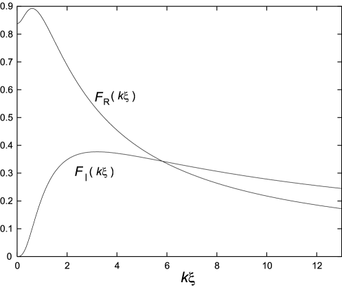
Figure 3: Two scaling functions corresponding to form birefringence and dichroism [8]. The $k$ is the wave number of probing light and $\xi$ is the correlation length.

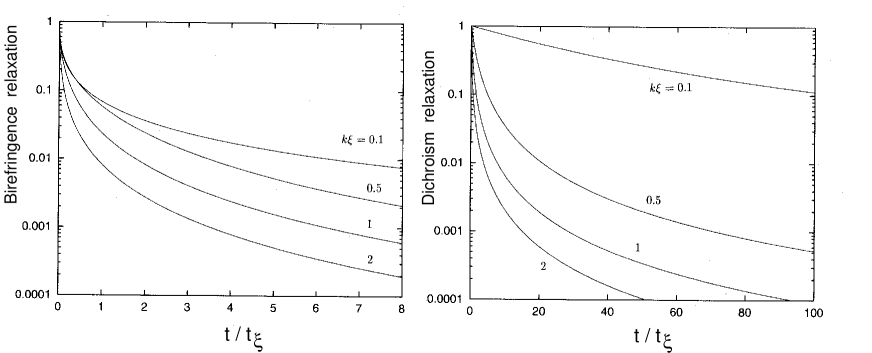
Figure 4: Normalized birefringence ${\rm Re}\Delta n(t)/{\rm Re}\Delta n(0)$ and dichroism ${\rm Im}\Delta n(t)/{\rm Im}\Delta n(0)$ vs $t/t_{\xi}$ on semilogarithmic scales for $k\xi=0.1,0.5,1$, and 2.

The anisotropy of the structure factor in (3.17) has not yet been measured in near-critical fluids, but it gives rise to critical anomaly in electric birefringence (Kerr effect) $[16$-$19]$ and dichroism. These effects can be sensitively detected even in the weak field regime $\tau_{\rm e}\ll\tau$ and even for not large $\varepsilon_{1}$ using high-sensitivity optical techniques. We assume that a laser beam with optical frequency $\omega$ is passing through a near-critical fluid along the $x$ axis, while an electric field $E_{0}$ is applied along the $z$ axis. In (1.5) we have $\Delta\varepsilon_{yz}=0$ and the difference $\Delta n=(\Delta\varepsilon_{zz}-\Delta\varepsilon_{yy})/2n(\omega)$ is written as [23, 24]

$$\Delta n=\frac{A_{{\rm op}}}{2n(\omega)}\int_{\mbox{\boldmath$q$}}\frac{q_{y}^{2}-q_{z}^{2}}{q^{2}-k^{2}-i0}I({\mbox{\boldmath$k$}}-{\mbox{\boldmath$q$}}),$$ (3.36)

where $k=\omega/n(\omega)$ is the laser wave number in the fluid and

$$A_{{\rm op}}=(\partial\varepsilon(\omega)/\partial\psi)^{2}/\varepsilon(\omega).$$ (3.37)

Here $A_{{\rm op}}$ is different from the static coefficient $A_{\rm s}$ in (3.14). In fact $A_{\rm op}\ll A_{\rm s}$ for polar fluid mixtures where $\varepsilon(0)\gg\varepsilon(\omega)$ at optical frequency $\omega$ [40]. When $\tau\gg\tau_{{\rm e}}$, substitution of (3.18) into (3.36) gives the steady state result,

$$\Delta n=\frac{A_{{\rm op}}}{32\pi^{2}n(\omega)}K_{0}^{-2}g_{{\rm e}}\xi\bigg{[}F_{\rm R}(k\xi)+iF_{\rm I}(k\xi)\bigg{]},$$ (3.38)

where the two scaling functions are plotted in Fig.3 and are given by

$$F_{\rm R}(x) = \frac{\pi}{4x^{2}}\bigg{(}1+\frac{1}{4x^{2}}\bigg{)}\bigg{[}\bigg{(}\frac{3}{2x}+2x\bigg{)}\tan^{-1}(2x)-3\bigg{]},$$

$$F_{\rm I}(x) = \frac{\pi}{4x}\bigg{[}\bigg{(}1+\frac{1}{x^{2}}+\frac{3}{16x^{2}}\bigg{)}\ln(1+4x^{2})-\frac{3}{4x^{2}}-\frac{5}{2}\bigg{]}.$$ (3.39)

For $x\ll 1$ we have $F_{\rm R}(x)\cong 4\pi/15$ and $F_{\rm I}(x)\cong\pi x^{3}/3$. In the long wavelength limit ($k\xi\ll 1$), we find $\Delta\varepsilon_{\rm eff}/n(\omega)\Delta n=3(A_{\rm s}-5\varepsilon_{2}/6)/A_{{\rm op}}$ from (3.29) and (3.38), so $\Delta\varepsilon_{\rm eff}$ and $\lim_{k\xi\rightarrow 0}\Delta n$ should have the same critical behavior. Experimentally, however, $\Delta n\propto\tau^{-z_{{\rm op}}}$ with $z_{{\rm op}}\cong 0.65-0.85>z_{\rm non}$ was obtained [14, 18].

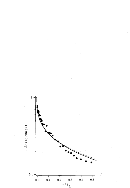
Figure 5: Comparison of the theoretical decay function (bold line) defined by (3.41) and data (dots) taken from Ref.[18]. The stretched exponential function $\exp(-2.3x^{1/3})$ (dotted line) is a good approximation in the initial relaxation.

In transient electric birefringence, applied electric field is switched off (at $t=0$) and the subsequent relaxation $\Delta n(t)$ (for $t>0$) is measured. For near-critical binary mixtures, this experiment has been carried out by applying a rectangular pulse of electric field $[16$-$19]$. If the pulse duration time $\Delta t$ is much longer than the relaxation time $t_{\xi}$ of the critical fluctuations, the fluid can reach a steady state while the field is applied. Here $t_{\xi}=6\pi{\bar{\eta}}\xi^{3}/k_{\rm B}T_{\rm c}$ with ${\bar{\eta}}$ being the shear viscosity. A remarkable finding is that $\Delta n(t)$ follows a stretched exponential relaxation at short times. We hereafter explain our theory for weak field $\tau_{\rm e}\ll\tau$ [8].

We assume that the relaxation of the structure factor obeys

$$I({\mbox{\boldmath$q$}},t)=I_{0}(q)-I_{0}(q)^{2}g_{\rm e}\hat{q}_{z}^{2}\exp(-2\Gamma_{q}t)+\cdots,$$ (3.40)

where $\Gamma_{q}=t_{\xi}^{-1}K_{0}(q\xi)$ is the relaxation rate with $K_{0}(x)=(3/4)[1+x^{2}+(x^{3}-x^{-1})\tan^{-1}x]$ being the Kawasaki function [22]. Thus $\Gamma_{q}=Dq^{2}$ for $q\xi\ll 1$ with the diffusion constant $D=k_{\rm B}T_{\rm c}/6\pi{\bar{\eta}}\xi$. Here we neglect the term proportional to $\tau_{\rm c}$ in (3.18) because it does not contribute to $\Delta n$. We substitute (3.40) into (3.36) to obtain $\Delta n(t)$ as a function of $k\xi$ and $t/t_{\xi}$, where the initial value $\Delta n(0)$ is given by (3.38). In Fig.4 we plot its normalized real and imaginary parts for various $k\xi$. The imaginary part decays slower than the real part. In the limit $k\xi\rightarrow 0$, it becomes real and is of the form,

$$\lim_{k\xi\rightarrow 0}\frac{\Delta n(t)}{\Delta n(0)}=G(t/t_{\xi})=\frac{4}{\pi}\int^{\infty}_{0}dy{y^{2}\over(1+y^{2})^{2}}\exp[-2K_{0}(y)t/t_{\xi}],$$ (3.41)

where the scaling function $G(x)$ behaves as

$$G(x) \cong 1-2.3x^{1/3}\cong\exp(-2.3x^{1/3})\quad\qquad(x\ll 1)$$ (3.42)

$$\cong 0.2x^{-3/2}~{}\hskip 85.35826pt\quad\quad\qquad(x\gg 1).$$

In Fig.5 data on butoxyetbaranol + water [18] are compared with (3.41) for $t<t_{\xi}$. The agreement is excellent. It demonstrates that the theoretical $G(t)$ is nearly stretched-exponential for $G(t)>\kern-12.0pt\lower 5.0pt\hbox{$\displaystyle{\sim}$}0.1$ or for $t/t_{\xi}<\kern-12.0pt\lower 5.0pt\hbox{$\displaystyle{\sim}$}0.5$. As another theory, Piazza et al. [17] derived a stretched exponential decay of $\Delta n(t)$ on the basis of a phenomenological picture on the distribution of large clusters.

Let us consider the case $k\xi\ll 1$, where (3.41) is a good approximation for $t<\kern-12.0pt\lower 5.0pt\hbox{$\displaystyle{\sim}$}1/Dk^{2}$. At $t\sim 1/Dk^{2}$, $G(t/t_{\xi})$ becomes a very small number of order $0.2(k\xi)^{3}$. In the later time region $t>\kern-12.0pt\lower 5.0pt\hbox{$\displaystyle{\sim}$}(Dk^{2})^{-1}$, (3.41) cannot be used and the fluctuations with wave numbers of order $(Dt)^{-1/2}$ give rise to the following birefringence signal,

$$\frac{{\rm Re}\Delta n(t)}{{\rm Re}\Delta n(0)}\cong 0.2(t/t_{\xi})^{-3/2}(Dk^{2}t)^{-1}.$$ (3.43)

Data of birefringence relaxation in Ref.[19] indicated that the decay becomes faster than predicted by (3.41) at long times. The same tendency can be seen in Fig.4. In future such data should be compared with the theoretical curves for finite $k\xi$. We note that transient electric dichroism has not yet been measured for near-critical fluids, but was measured for a polymer solution[27].

3.6 Interface instability induced by electric field

An interface between two immiscible fluids becomes unstable against surface undulations in perpendicularly applied electric field. This is because the electrostatic energy is higher for perpendicular field than for parallel field. In classic papers [37] the instability on an interface between conducting and nonconducting fluids (such as Hg and air) was treated. In helium systems, where an interface can be charged with ions, the critical field is much decreased and intriguing surface patterns have been observed [38].

We will derive this instability in the simplest manner [39]. Let a planar interface be placed at $z=z_{0}$ in a near-critical fluid without ions in weak field, $\tau<0$ and $|\tau|\gg\tau_{\rm e}$. If the interface is displaced by a small height $\zeta(x,y)$, we may set ${\partial}\psi/\partial z=\Delta\psi\delta(z-z_{0}-\zeta)$ in (3.13), where $\Delta\psi$ is the order parameter difference between the two phases. This means that the effective surface charge density is given by $-\varepsilon_{1}\Delta\psi E_{0}$. If $z_{0}$ is far from the boundaries, we obtain

$${F}_{\rm dip}=\frac{1}{8\pi}C_{\rm e}{\int}d{\mbox{\boldmath$r$}}_{\perp}{\int}d{\mbox{\boldmath$r$}}^{\prime}_{\perp}[|{\zeta({\mbox{\boldmath$r$}}_{\perp})-\zeta({\mbox{\boldmath$r$}}^{\prime}_{\perp})|^{2}+|{\mbox{\boldmath$r$}}_{\perp}-{\mbox{\boldmath$r$}}^{\prime}_{\perp}|^{2}}]^{-1/2},$$ (3.44)

where ${\mbox{\boldmath$r$}}_{\perp}=(x,y)$, ${{\mbox{\boldmath$r$}}}^{\prime}_{\perp}=(x^{\prime},y^{\prime})$, and

$$C_{\rm e}=A_{\rm s}E_{0}^{2}(\Delta\psi)^{2}/4\pi.$$ (3.45)

We expand the integrand of (3.44) in powers of $[\zeta({\mbox{\boldmath$r$}}_{\perp})-\zeta({{\mbox{\boldmath$r$}}_{\perp}}^{\prime})]^{2}$. The first correction is negative and bilinear in $\zeta$. In terms of the Fourier transformation $\zeta_{\small{\mbox{\boldmath$k$}}}$ we have

$$\Delta{F}_{\rm dip} = -\frac{1}{16\pi}C_{\rm e}{\int}d{{\mbox{\boldmath$r$}}}_{\perp}{\int}d{{\mbox{\boldmath$r$}}}^{\prime}_{\perp}\frac{1}{{|}{{\mbox{\boldmath$r$}}}_{\perp}-{{{\mbox{\boldmath$r$}}}_{\perp}}^{\prime}{|}^{3}}\left[\zeta({\mbox{\boldmath$r$}}_{\perp})-\zeta({{\mbox{\boldmath$r$}}}^{\prime}_{\perp})\right]^{2}$$ (3.46)

$$= -\frac{1}{2}C_{\rm e}{\int}_{\mbox{\boldmath$k$}}k\mid\zeta_{\small{\mbox{\boldmath$k$}}}\mid^{2},$$

where $k$ is the two-dimensional wave vector with $k=|{\mbox{\boldmath$k$}}|$ and $\int_{\mbox{\boldmath$k$}}=(2\pi)^{-2}\int d{\mbox{\boldmath$k$}}$. We have used the formula ${\int}d{{\mbox{\boldmath$r$}}}_{\perp}[1-\exp(i{\small{\mbox{\boldmath$k$}}}\cdot{{\mbox{\boldmath$r$}}}_{\perp})]/r_{\perp}^{3/2}=4\pi k$. Including gravity we write the total free energy change due to the surface deformation as

$$\Delta F_{\rm surface}=\frac{1}{2}\int_{\mbox{\boldmath$k$}}[\sigma k^{2}+g\Delta\rho-C_{\rm e}k]\mid\zeta_{\small{\mbox{\boldmath$k$}}}\mid^{2},$$ (3.47)

where $\sigma$ is the surface tension, $g$ is the gravitational acceleration, and $\Delta\rho$ is the mass density difference between the two phases. The coefficient in front of $\mid\zeta_{\small{\mbox{\boldmath$k$}}}\mid^{2}$ is minimum at $k=(C_{\rm e}/2\sigma)^{1/2}$ and an instability is triggered for $C_{\rm e}>2(\sigma g\Delta\rho)^{1/2}$. For polar mixtures this criterion is typically $E_{0}>|\tau|^{\nu/2-3\beta/4}$kV$/$cm on earth.

4 Near-critical fluids with ions

We will discuss the effects of ions doped in binary mixtures. It has long been known that even a small fraction of ions (salt) with $c\ll 1$ dramatically changes the liquid-liquid phase behavior in polar binary mixtures, where $c$ is the mass or mole fraction of ions. For small $c$, the UCST coexistence curve shifts upward as

$$(\Delta T)_{\rm c}=A_{1}c+O(c^{2})$$ (4.1)

with large positive coefficient $A_{1}$, expanding the region of demixing. For example, $A_{1}/T_{\rm c}\sim 10$ with $T_{\rm c}\sim 300$K when NaCl was added to cyclohexane$+$methyl alcohol [41] and to triethylamine+water [42]. Similar large impurity effects were observed when water was added to methanol+cyclohexane [43]. In some polar mixtures, even if they are miscible at all $T$ at atmosphere pressure without salt, addition of a small amount of salt gives rise to reentrant phase separation behavior [44, 45].

We consider two species of ions with charges, $Ze$ and $-e$, at very low densities, $n_{1}({\mbox{\boldmath$r$}})$ and $n_{2}({\mbox{\boldmath$r$}})$, in a near-critical binary mixture. The average densities are written as $\langle{n_{1}}\rangle_{\rm s}={\bar{n}}$ and $\langle{n_{2}}\rangle_{\rm s}=Z{\bar{n}}$, where $\langle{\cdots}\rangle_{\rm s}$ denotes taking the space average. The charge neutrality condition yields $Z\langle{n_{1}}\rangle_{\rm s}=\langle{n_{2}}\rangle_{\rm s}$. The Debye wave number $\kappa$ and the Bjerrum length $\ell_{\rm B}$($=7\AA$ for water at $300$K) are defined by

$$\kappa=[4\pi(Z^{2}+Z)\bar{n}e^{2}/\varepsilon k_{\rm B}T]^{1/2},\quad\ell_{\rm B}=e^{2}/\varepsilon k_{\rm B}T.$$ (4.2)

4.1 Ginzburg-Landau theory

We set ${\mbox{\boldmath$p$}}={\chi}(\psi){\mbox{\boldmath$E$}}$ from the beginning. Then the electric potential $\phi$ satisfies $-\nabla\cdot\varepsilon\nabla{\phi}=4\pi\rho$ with $\varepsilon=1+4\pi\chi$ and $\rho=e(Zn_{1}-n_{2})$. We assume that the free energy $F$ in (2.2) in the fixed charge condition is of the form,

$$F=F_{0}\{\psi\}+k_{\rm B}T\int d{\mbox{\boldmath$r$}}\bigg{[}n_{1}\ln n_{1}+n_{2}\ln n_{2}+(w_{1}n_{1}+w_{2}n_{2})\psi\bigg{]}+\frac{1}{8\pi}\int d{\mbox{\boldmath$r$}}\varepsilon{\mbox{\boldmath$E$}}^{2},$$ (4.3)

where the first term depends only on $\psi$ and is given by (3.2), and the terms proportional to $w_{1}$ and $w_{2}$ arise from an energy decrease due to microscopic polarization of the fluid around individual ions. In the neighborhood of an ion of species $\alpha$ $(\alpha=1,2$), the electric field and the polarization are given by ${\mbox{\boldmath$E$}}_{\rm ind}=-\nabla(Z_{\alpha}e/\varepsilon r)$ and ${\mbox{\boldmath$p$}}_{\rm ind}=\chi{\mbox{\boldmath$E$}}_{\rm ind}$ in terms of the local $\chi$ and $\varepsilon$, where we write $Z_{1}=Z$ and $Z_{2}=-1$. The resultant electrostatic energy density is localized near the ion $(\propto r^{-4}$) and its space integral is $\int d{\mbox{\boldmath$r$}}\varepsilon{\mbox{\boldmath$E$}}_{\rm ind}^{2}/8\pi=Z_{\alpha}^{2}e^{2}/2\varepsilon r_{\alpha}$, where $r_{\alpha}$ is the lower cutoff representing an effective radius of an ion of species $\alpha$. Here the screening length is assumed to be much longer than $r_{\alpha}$. Due to the polarization, the decrease of the electrostatic energy (solvation free energy per ion) is given by the Born formula[40, 46],

$$\Delta E_{\alpha}=(1/\varepsilon-1)Z_{\alpha}^{2}e^{2}/2r_{\alpha}.$$ (4.4)

Neglecting $\psi$-dependence of $r_{\alpha}$ we estimate $w_{\alpha}$ as

$$w_{\alpha}=(k_{\rm B}T)^{-1}\frac{\partial}{\partial\psi}(\Delta E_{\alpha})=-\varepsilon_{1}Z_{\alpha}^{2}\ell_{\rm B}/2\varepsilon_{0}r_{\alpha}.$$ (4.5)

The last term in (4.3) is the electrostatic free energy $\Delta F$ arising from slowly-varying fluctuations and depends on the boundary condition. As a clear illustration, if all the quantities are functions of $z$ only in the charge-fixed condition, we have

$$\Delta F=2\pi S\int_{0}^{L}dz[\sigma_{\rm ex}-w(z)]^{2}/\varepsilon(z),$$ (4.6)

where $\sigma_{\rm ex}$ is the capacitor charge density and $w(z)=\int_{0}^{z}dz^{\prime}\rho(z^{\prime})$. Though neglected here, electrostriction should also be investigated around charged particles (see Subsection 3.4), which can well produce a shift of the critical composition.

In this model the chemical potentials $\mu_{\alpha}=\delta F/\delta n_{\alpha}$ of the ions are given by

$$\mu_{\alpha}=k_{\rm B}T(\ln n_{\alpha}+1+w_{\alpha}\psi)+Z_{\alpha}e\phi.$$ (4.7)

In equilibrium $\mu_{\alpha}$ become homogeneous, leading to ion distributions,

$$n_{\alpha}({\mbox{\boldmath$r$}}) = n_{\alpha 0}\exp[-w_{\alpha}\psi({\mbox{\boldmath$r$}})-Z_{\alpha}e\phi({\mbox{\boldmath$r$}})/k_{\rm B}T]$$ (4.8)

$$\cong n_{\alpha 0}[1-w_{\alpha}\psi({\mbox{\boldmath$r$}})-Z_{\alpha}e\phi({\mbox{\boldmath$r$}})/k_{\rm B}T].$$

The second line holds when the exponents in the first line are small. Let us use the second line to derive Debye-H$\ddot{\rm u}$ckel-type relations. Then $n_{\alpha 0}\cong\langle{n_{\alpha}}\rangle_{\rm s}[1+w_{\alpha}\langle{\psi}\rangle_{\rm s}+Z_{\alpha}e\langle{\phi}\rangle_{\rm s}/k_{\rm B}T]$. The potential $\phi$ satisfies

$$\varepsilon_{0}(\kappa^{2}-\nabla^{2})\phi=\varepsilon_{1}\nabla\psi\cdot\nabla\phi+{4\pi}e[Zn_{10}-n_{20}-Z{\bar{n}}(w_{1}-w_{2})\psi].$$ (4.9)

The right hand side consists of new contributions dependent on $\psi$, where the first term is important in the presence of applied field. We here notice the following.
(i) In applied electric field we can examine the ions distribution accumulated near the boundaries using (2.4) and (4.8) (or (4.9)).
(ii) When $w_{1}\neq w_{2}$, charge distributions arise around domains or wetting layers. Let the interface thickness ($\sim\xi$) be shorter than the Debye length $\kappa^{-1}$. For a spherical domain with radius $R$, for example, the electric potential $\phi(r)$ is a function of the distance $r$ from the center of the sphere and then

$$\Delta\phi=\phi(0)-\phi(\infty)=[1-e^{-\kappa R}(1+\kappa R)]\Phi_{\rm sat}.$$ (4.10)

For $\kappa R\gg 1$, $\Delta\phi$ saturates into

$$\Phi_{\rm sat}=-[k_{\rm B}T/e(Z+1)](w_{1}-w_{2})\Delta\psi,$$ (4.11)

where $\Delta\psi$ is the difference of $\psi$ between the two phases. For $\kappa R\ll 1$ we find $\Delta\phi\cong(\kappa R)^{2}\Phi_{\rm sat}$. The same potential difference $\Phi_{\rm sat}$ arises across a planar interface. For example, if $w_{1}-w_{2}\sim 3$, $Z=1$, and $\Delta\psi\sim 10^{-1}$, we have $|\Phi_{\rm sat}|\sim 10^{-2}$V.
(iii) In slow relaxation of $\delta\psi$, the deviations $\delta\mu_{\alpha}=k_{\rm B}T(\delta n_{\alpha}/\langle{n_{\alpha}}\rangle_{\rm s}+w_{\alpha}\delta\psi)+Z_{\alpha}e\delta\phi$ should quickly relax to zero. Then the deviations $\delta n_{\alpha}$ are written in terms of $\delta\psi$ as

$$\delta n_{1}+\delta n_{2}=-{\bar{n}}(w_{1}+Zw_{2})\delta\psi,$$ (4.12)

$$(\kappa^{2}-\nabla^{2})\rho=\bigg{[}Ze\bar{n}(w_{1}-w_{2})\nabla^{2}+\frac{1}{4\pi}\varepsilon_{1}\kappa^{2}{\bf E}_{0}\cdot\nabla\bigg{]}\delta\psi,$$ (4.13)

where we allow the presence of electric field $E_{0}$ to derive (4.22) below.

4.2 Ion effects on phase transition

We consider small fluctuations in a one-phase state without electric field ($E_{0}=0)$. The fluctuation contributions to $F$ in the bilinear order are written as

$$\frac{\delta F}{k_{\rm B}T} = \int_{\mbox{\boldmath$q$}}\bigg{[}\frac{1}{2}({a_{0}\tau+C_{0}q^{2}})|\psi_{\small{\mbox{\boldmath$q$}}}|^{2}+\sum_{\alpha=1,2}\bigg{(}\frac{|n_{\alpha{\small{\mbox{\boldmath$q$}}}}|^{2}}{2\langle{n_{\alpha}}\rangle_{\rm s}}+w_{\alpha}n_{\alpha{\small{\mbox{\boldmath$q$}}}}\psi_{\small{\mbox{\boldmath$q$}}}^{*}\bigg{)}+\frac{2\pi}{k_{\rm B}T\varepsilon_{0}q^{2}}|\rho_{\small{\mbox{\boldmath$q$}}}|^{2}\bigg{]}$$ (4.14)

$$= \frac{1}{2}\int_{{\mbox{\boldmath$q$}}}\bigg{[}a_{0}\tau+C_{0}q^{2}-\frac{\bar{n}(w_{1}+Zw_{2})^{2}}{1+Z}-\frac{Z\bar{n}(w_{1}-w_{2})^{2}}{(1+Z)(q^{2}+\kappa^{2})}{q^{2}}\bigg{]}|\psi_{\small{\mbox{\boldmath$q$}}}|^{2}.$$

In the first line $n_{\alpha{\small{\mbox{\boldmath$q$}}}}$ and $\rho_{\small{\mbox{\boldmath$q$}}}$ are the Fourier transformations of $\delta n_{\alpha}=n_{\alpha}-\langle{n_{\alpha}}\rangle_{\rm s}$ and the charge density $\rho=e(Zn_{1}-n_{2})$. In the second line we have expressed $n_{\alpha{\small{\mbox{\boldmath$q$}}}}$ in terms of $\psi_{\small{\mbox{\boldmath$q$}}}$ using (4.12) and (4.13) and minimized the first line. We introduce a parameter,

$$\gamma_{\rm p}=|w_{1}-w_{2}|/[(1+Z)(4\pi C_{0}\ell_{\rm B})^{1/2}].$$ (4.15)

This number is independent of the ion density and represents the strength of asymmetry in the ion-induced polarization between the two components. The structure factor at $E_{0}=0$ in the mean field theory is written as

$$1/I_{0}(q)=a_{0}(\tau-\tau_{\rm ion})+C_{0}q^{2}[1-\gamma_{\rm p}^{2}\kappa^{2}/(q^{2}+\kappa^{2})],$$ (4.16)

where

$$\tau_{\rm ion}=(w_{1}+Zw_{2})^{2}\bar{n}/(1+Z){a_{0}}.$$ (4.17)

We draw the following conclusions.
(i) If $\gamma_{\rm p}<1$, $I_{0}(q)$ is maximum at $q=0$ and the critical temperature shift due to ions is given by $T_{\rm c}\tau_{\rm ion}$ in the form of (4.1). As a rough estimate for $Z=1$, we set $a_{0}^{-1}\bar{n}\sim\xi_{+0}^{3}\bar{n}\sim{c}$, where $c$ is the mass or mole fraction. Then $\tau_{\rm ion}\sim(w_{1}+w_{2})^{2}{c}$. If $|w_{1}+w_{2}|\sim 3$, this result is consistent with the experiments [41, 42]. In future experiments let $1/C_{0}I_{0}(q)$ vs $q^{2}$ be plotted; then, the slope is $1-\gamma_{\rm p}^{2}$ for $q\ll\kappa$ and is $1$ for $q\gg\kappa$. This changeover is detectable unless $\gamma_{\rm p}\ll 1$.
(ii) The case $\gamma_{\rm p}=1$ corresponds to a so-called Lifshitz point [47], where $1/I(q)-1/I(0)\propto q^{4}/(q^{2}+\kappa^{2})$.
(iii) If $\gamma_{\rm p}>1$, the structure factor attains a maximum at an intermediate wave number $q_{\rm m}$ given by

$$q_{\rm m}=(\gamma_{\rm p}-1)^{1/2}\kappa\propto{\bar{n}}^{1/2}.$$ (4.18)

The maximum structure factor $I_{0}(q_{\rm m})$ diverges as $\tau\rightarrow\tau_{\rm ion}^{\prime}$, where

$$\tau_{\rm ion}^{\prime}=\tau_{\rm ion}+(\gamma_{\rm p}-1)^{2}\xi_{+0}^{2}\kappa^{2},$$ (4.19)

with the aid of $C_{0}=a_{0}\xi_{+0}^{2}$. A charge-density-wave phase should be realized for $\tau<\tau_{\rm ion}^{\prime}$. It is remarkable that this mesoscopic phase appears however small $\bar{n}$ is (as long as $\gamma_{\rm p}>1$ and $q_{\rm m}L\gg 1$, $L$ being the system length). Here relevant is the coupling of the order parameter and the charge density in the form $\propto\psi\rho$ in the free energy density, which generally exists in ionic systems. This possibility of a mesoscopic phase was already predicted for electrolytes [48], but has not yet been confirmed in experiments.

Furthermore, we note that $\gamma_{p}$ increases with increasing $Z$. As an extreme case, we may add charged colloid particles with $Z\gg 1$ and radius $R$ in a near-critical polar mixture, where $w_{1}$ grows as $Z^{2}$ from (4.5) and

$$\gamma_{\rm p}\cong(\ell_{\rm B}/16\pi C_{0})^{1/2}(\varepsilon_{1}/\varepsilon_{0})Z/R.$$ (4.20)

Note that $Z\xi_{+0}/R$ can be made considerably larger than 1 with increasing $R$. Notice that the ionizable points on the surface is proportional to the surface area $4\pi R^{2}$.

4.3 Nonlinear effects under electric field

In most of the previous experiments, a pulse of strong electric field has been applied. For example, the field strength was $E_{0}=10^{4}$V$/$cm and the pulse duration time was $\Delta t=1$ms at $T\sim 300$K [13, 15]. Let us set $Z=1$. As can be seen from the general relation (2.18), we can neglect ion accumulation at the capacitor plates if

$$\sigma_{\rm ex}=\varepsilon E_{0}/4\pi\gg e{\bar{n}}v_{\rm dri}\Delta t\quad{\rm or}\quad\Delta t\ll t_{\rm dri}.$$ (4.21)

Here $v_{\rm dri}=\zeta^{-1}eE_{0}$ is the drift velocity, $\zeta$ is the friction coefficient related to the diffusion constant by $D_{\rm i}=k_{\rm B}T/\zeta$, and $t_{\rm dri}=(\kappa^{2}D_{\rm i})^{-1}$ is the drift time. For $\Delta t>t_{\rm dri}$ the electric field far from the boundaries are shielded if $\sigma_{\rm ex}<e{\bar{n}}L$. Typical experimental values are $D_{\rm i}\sim 10^{-6}$cm${}^{2}/$s, $\zeta\sim 10^{-8}$g$/$s, $\varepsilon\sim 50$, and $E_{0}=10^{4}$V$/$cm, leading to $v_{\rm dri}\sim 1$ cm$/$s. Then the condition (4.21) becomes ${\bar{n}}\Delta t\ll 10^{12}$cm^-3s and can well hold in experiments [49]. Under this condition and in a one-phase state, the bulk region remains homogeneous and the electric field is not yet shielded. If we are interested in slow motions of $\psi$, we may assume (4.12) and (4.13) to obtain the decay rate of $\psi_{\small{\mbox{\boldmath$q$}}}$ in the form $\Gamma_{\small{\mbox{\boldmath$q$}}}=L_{0}q^{2}/I({\mbox{\boldmath$q$}})$ ($L_{0}$ being the kinetic coefficient) with

$${I({\mbox{\boldmath$q$}})}^{-1}={I_{0}(q)}^{-1}+[-{\varepsilon_{2}}+A_{\rm s}{q_{z}^{2}}/({q^{2}+\kappa^{2}})](E_{0}^{2}/4\pi k_{\rm B}T),$$ (4.22)

where $I_{0}(q)$ is given by (4.16). If the pulse duration time $\Delta t$ is much longer than the relaxation time $1/\Gamma_{\small{\mbox{\boldmath$q$}}}$, the structure factor is given by $I({\mbox{\boldmath$q$}})$. Here ${\hat{q}}_{z}^{2}=q_{z}^{2}/q^{2}$ in (3.17) is replaced by ${q_{z}^{2}}/({q^{2}+\kappa^{2}})$ in the presence of ions due to the Debye screening. Let us consider the nonlinear dielectric constant in (3.29) and the electric birefringence $\lim_{k\xi\rightarrow 0}\Delta n$ in (3.36) on the order of $E_{0}^{2}$. For $\kappa\xi<1$ the ion effect is small, but for $\kappa\xi>1$ they should behave as

$$\Delta\varepsilon_{\rm eff}/A_{\rm s}\sim\Delta n/A_{\rm op}\propto E_{0}^{2}\kappa^{-1}.$$ (4.23)

This crossover occurs for $c\sim{\bar{n}}\xi_{+0}^{3}>\tau^{2\nu}$ in the weak field regime $\tau\gg\tau_{\rm e}$.

We also comment on the Joule heating. While the ions are drifting, the temperature increasing rate is given by

$$C\frac{d}{dt}T=2{\bar{n}}v_{\rm dri}eE_{0}=2{\bar{n}}e^{2}E_{0}^{2}/\zeta=\varepsilon E_{0}^{2}/4\pi t_{\rm dri},$$ (4.24)

where $C$ is the specific heat per unit volume at constant volume and composition. For $\Delta t>t_{\rm dri}$ the temperature will increase by $(\Delta T)_{\rm Joule}\sim\varepsilon E_{0}^{2}/4\pi C$. By setting $C\sim k_{\rm B}\xi_{+0}^{-3}$, we obtain $d\tau/dt\sim 10^{-19}{\bar{n}}\sim 10^{-6}t_{\rm dri}^{-1}$ s^-1 at $E_{0}=10^{4}$V$/$cm. The heating is negligible for very small ${\bar{n}}\Delta t$ or for not very small $\tau$.

As other nonlinear problems involving ions, we mention transient relaxation of the charge distribution after application of dc field, response to oscillating field, and effects of charges on wetting layers and interfaces between the two phases.

5 Liquid crystals in electric field

In liquid crystals near the isotropic-nematic transition, the order parameter is the symmetric, traceless, orientation tensor $\psi={\{}Q_{ij}\}$ (which should be distinguished from the electric charge $Q$ on a capacitor plate). The polarization and the electric induction are written as ${\mbox{\boldmath$p$}}=\stackrel{{\scriptstyle\leftrightarrow}}{{{{\chi}}}}\cdot{\mbox{\boldmath$E$}}$ and ${\mbox{\boldmath$D$}}=\stackrel{{\scriptstyle\leftrightarrow}}{{{\varepsilon}}}\cdot{\mbox{\boldmath$E$}}$, respectively, where the polarizability tensor $\stackrel{{\scriptstyle\leftrightarrow}}{{{{\chi}}}}$ depends on $Q_{ij}$ and the local dielectric tensor $\stackrel{{\scriptstyle\leftrightarrow}}{{{\varepsilon}}}=1+4\pi\stackrel{{\scriptstyle\leftrightarrow}}{{{\chi}}}$ reads

$$\varepsilon_{ij}=\varepsilon_{0}\delta_{ij}+\varepsilon_{1}Q_{ij}+\varepsilon_{21}Q^{2}\delta_{ij}+\varepsilon_{22}(Q^{2})_{ij}+\cdots,$$ (5.1)

where $Q^{2}=\sum_{ij}Q^{2}_{ij}$ hereafter. In the nematic phase we may set $Q_{ij}=S(n_{i}n_{j}-\delta_{ij}/3)$ in terms of the amplitude $S$ and the director $n$. Then,

$$\varepsilon_{ij}=\varepsilon_{0}^{\prime}(S)\delta_{ij}+\varepsilon_{1}^{\prime}(S)n_{i}n_{j},$$ (5.2)

where $\varepsilon_{0}^{\prime}=\varepsilon_{0}+S^{2}(2\varepsilon_{21}/3+\varepsilon_{22}/9)$ and $\varepsilon_{1}^{\prime}=\varepsilon_{1}S+\varepsilon_{22}S^{2}/3$. These relations are analogous to (1.2) for near-critical fluids. An important difference is that the tensor ${\{}Q_{ij}\}$ is not conserved and its average is sensitive to applied electric field, while the average order parameter in near-critical fluids is fixed or conserved.

5.1 Pretransitional growth

Here we examine the effect of the field-induced dipolar interaction. If we assume no mobile charges inside the fluid, the free energy functional is given by $F=F_{0}+\int d{\mbox{\boldmath$r$}}{\mbox{\boldmath$E$}}\cdot{\mbox{\boldmath$D$}}/8\pi$ at fixed capacitor charge, where

$$F_{0}=\int d{\mbox{\boldmath$r$}}[\frac{A(T)}{2}Q^{2}+\lambda\sum_{j}Q_{jj}+\frac{L_{1}}{2}\sum_{ijk}[\nabla_{k}Q_{ij}]^{2}+\frac{L_{2}}{2}\sum_{ijk}\nabla_{i}Q_{ij}\nabla_{k}Q_{kj}+\cdots]$$ (5.3)

is the Ginzburg-Landau free energy for ${\{}Q_{ij}\}$ and $\lambda$ is a space-dependent Legendre multiplier ensuring $\sum_{j}Q_{jj}=0$ [20]. For weakly first order phase transition, the coefficient $A(T)=a_{1}(T-T_{0})$ becomes small as $T$ approaches $T_{0}$. In $F_{0}$ the higher order terms are not written explicitly. Analogously to (3.9) we find

$$\delta F=\delta F_{0}-\int d{\mbox{\boldmath$r$}}{\mbox{\boldmath$E$}}\cdot\delta{\stackrel{{\scriptstyle\leftrightarrow}}{{{\varepsilon}}}}\cdot{\mbox{\boldmath$E$}}/8\pi.$$ (5.4)

Thus,

$$\frac{\delta}{\delta Q_{ij}}F=[A(T)Q_{ij}+\lambda\delta_{ij}+\cdots]-\frac{\varepsilon_{1}}{8\pi}E_{i}E_{j},$$ (5.5)

where the gradient term is omitted. At fixed capacitor potential, on the other hand, the appropriate free energy is $G=F_{0}-\int d{\mbox{\boldmath$r$}}{\mbox{\boldmath$E$}}\cdot{\mbox{\boldmath$D$}}/8\pi$ but $\delta G/\delta Q_{ij}$ is of the same form as $\delta F/\delta Q_{ij}$ in (5.5). In equilibrium disordered states with $T>T_{0}$, we set $\langle{\delta F/\delta Q_{ij}}\rangle=0$ to obtain

$$\langle{Q_{ij}}\rangle=\frac{\varepsilon_{1}}{8\pi}(E_{0i}E_{0j}-\frac{1}{3}E_{0}^{2}\delta_{ij})\frac{1}{A(T)}+\cdots,$$ (5.6)

where ${\mbox{\boldmath$E$}}_{0}$ is the average electric field assumed to be along the $z$ axis. On the other hand, analogously to (3.27), the macroscopic static dielectric constant is given by

$$\varepsilon_{\rm eff}=\langle{{\varepsilon_{zz}}}\rangle-\int_{\mbox{\boldmath$q$}}\frac{1}{\varepsilon_{0}q^{2}}\langle{|\sum_{j}q_{j}{\varepsilon}_{jz}({\small{{\mbox{\boldmath$q$}}}})|^{2}}\rangle,$$ (5.7)

where ${{\varepsilon}_{ij}}({\small{{\mbox{\boldmath$q$}}}})$ are the Fourier transformation of ${{\varepsilon}}_{ij}({\mbox{\boldmath$r$}})$. As $T\rightarrow T_{0}$, the average $\langle{{\varepsilon_{zz}}}\rangle$ yields the dominant contribution to the nonlinear dielectric constant [20],

$$\Delta\varepsilon_{\rm eff}\cong\varepsilon_{1}^{2}E_{0}^{2}/12\pi{A(T)},$$ (5.8)

in agreement with the experiments [21]. The contribution from the second term in (5.7) is smaller than that in (5.8) by $(\varepsilon_{1}/\varepsilon_{0})^{2}k_{\rm B}TA(T)^{1/2}/L_{1}^{3/2}$ for $L_{2}\sim L_{1}$.

The electrostatic free energy $\Delta F=F-F_{0}$ up to of order $Q^{2}$ is written as

$$\Delta F=-\frac{E_{0}^{2}}{8\pi}\int d{\mbox{\boldmath$r$}}\varepsilon_{zz}(\stackrel{{\scriptstyle\leftrightarrow}}{{{Q}}})+A_{\rm s}\frac{E_{0}^{2}}{8\pi}\int_{\mbox{\boldmath$q$}}\frac{1}{q^{2}}|\sum_{j}{q_{j}}Q_{jz}({\mbox{\boldmath$q$}})|^{2},$$ (5.9)

where $A_{\rm s}=\varepsilon_{1}^{2}/\varepsilon_{0}$ and the dipolar interaction, the second term, is expressed in terms of the Fourier transformations $Q_{ij}({\mbox{\boldmath$q$}})$. The correlation functions of $Q_{ij}({\mbox{\boldmath$q$}})$ in disordered states depend on the direction $q^{-1}{\mbox{\boldmath$q$}}$ even in the limit $q\rightarrow 0$. For simplicity, for $q_{z}=0$ we obtain

$$\lim_{q\rightarrow 0}\langle{Q_{iz}({\mbox{\boldmath$q$}})Q_{jz}({\mbox{\boldmath$q$}})^{*}}\rangle=\frac{k_{\rm B}T}{r}\bigg{[}{\delta_{ij}}-\frac{q_{i}q_{j}}{q^{2}}\frac{r_{\rm e}}{r+r_{\rm e}}\bigg{]}\qquad(i,j=x,y),$$ (5.10)

where $r=2A(T)-(2\varepsilon_{21}+\varepsilon_{22})E_{0}^{2}/4\pi$ and $r_{\rm e}=A_{\rm s}E_{0}^{2}/4\pi$.

5.2 Director fluctuations in nematic states

We consider nematic states considerably below the transition, where we may neglect the fluctuations of the amplitude $S$ [20]. Hereafter we rewrite $\varepsilon_{0}^{\prime}$ and $\varepsilon_{1}^{\prime}$ in (5.2) as $\varepsilon_{0}$ and $\varepsilon_{1}$ for simplicity. If $\varepsilon_{0}$ is positive, the average orientation of the director can be along the $z$ axis from minimization of the first term in (5.8). Then the deviation $\delta{\mbox{\boldmath$n$}}$ perpendicular to the $z$ axis undergo large fluctuations at small wave numbers. In electric field $\Delta F$ in (5.9) becomes

$$\Delta F=\frac{1}{8\pi}E_{0}^{2}\int_{\mbox{\boldmath$q$}}\bigg{[}\varepsilon_{1}|\delta{\mbox{\boldmath$n$}}({\mbox{\boldmath$q$}})|^{2}+A_{\rm s}^{\prime}\frac{1}{q^{2}}|{\mbox{\boldmath$q$}}\cdot\delta{\mbox{\boldmath$n$}}({\mbox{\boldmath$q$}})|^{2}\bigg{]},$$ (5.11)

where $A_{\rm s}^{\prime}=A_{\rm s}S^{2}$. For general $q$ we obtain the correlation functions,

$$G_{ij}({\mbox{\boldmath$q$}})=\langle{\delta n_{i}({\mbox{\boldmath$q$}})\delta n_{j}({\mbox{\boldmath$q$}})^{*}}\rangle=k_{\rm B}T\frac{\delta_{ij}}{r_{2}}+k_{\rm B}T\frac{q_{i}q_{j}}{q_{\perp}^{2}}\bigg{(}\frac{1}{r_{1}}-\frac{1}{r_{2}}\bigg{)}\quad(i,j=x,y),$$ (5.12)

where $q_{\perp}^{2}=q_{x}^{2}+q_{y}^{2}$, and

$$r_{1}=K_{3}q_{z}^{2}+K_{1}q_{\perp}^{2}+\frac{1}{4\pi}\bigg{(}\varepsilon_{1}+A_{\rm s}^{\prime}\frac{q_{\perp}^{2}}{q^{2}}\bigg{)}E_{0}^{2},\quad r_{2}=K_{3}q_{z}^{2}+K_{2}q_{\perp}^{2}+\frac{1}{4\pi}\varepsilon_{1}E_{0}^{2}.$$ (5.13)

The $K_{1}$, $K_{2}$, and $K_{3}$ are the Frank constants. If $\varepsilon_{1}>\kern-12.0pt\lower 5.0pt\hbox{$\displaystyle{\sim}$}A_{\rm s}^{\prime}$, the correlation length $\xi$ is of the following order,

$$\xi\sim(4\pi K/\varepsilon_{1})^{1/2}E_{0}^{-1},$$ (5.14)

where $K$ represents the magnitude of the Frank constants and $k_{\rm B}T/K$ is a microscopic length. The scattered light intensity is proportional to the following [20],

$$\langle{|{\mbox{\boldmath$f$}}\cdot\stackrel{{\scriptstyle\leftrightarrow}}{{{\varepsilon}}}({\small{\mbox{\boldmath$q$}}})\cdot{\mbox{\boldmath$i$}}|^{2}}\rangle=k_{\rm B}T\varepsilon_{1}^{2}\bigg{[}|{\mbox{\boldmath$a$}}|^{2}/r_{2}+(1/r_{1}-1/r_{2})|{\mbox{\boldmath$q$}}\cdot{\mbox{\boldmath$a$}}|^{2}/{q_{\perp}^{2}}\bigg{]},$$ (5.15)

where $i$ and $f$ represent the initial and final polarizations. The vector $a$ is defined by

$$a_{x}=i_{z}f_{x}+f_{z}i_{x},\quad a_{y}=i_{z}f_{y}+f_{z}i_{y},\quad a_{z}=0.$$ (5.16)

If $A_{\rm s}^{\prime}>0$, the intensity depends on $q^{-1}{\mbox{\boldmath$q$}}$ even in the limit $q\rightarrow 0$.

In nematic states the average $\langle{\varepsilon_{ij}}\rangle$ is anisotropic, leading to large intrinsic birefringence. We here consider form dichroism arising from the director fluctuations, where the laser wave vector $k$ is along the $x$ axis and the average director is along the $z$ axis. We assume the relation $\varepsilon_{ij}=\varepsilon_{0}\delta_{ij}+\varepsilon_{1}n_{i}n_{j}$ at optical frequencies using the same notation as in (5.2). As a generalization of (1.5), the fluctuation contribution to the dielectric tensor for the electromagnetic waves is of the form,

$$\Delta{\stackrel{{\scriptstyle\leftrightarrow}}{{{{\varepsilon}}}}}=\frac{1}{\varepsilon_{0}}\int_{\mbox{\boldmath$q$}}\frac{1}{q^{2}-k^{2}-i0}\langle{[\stackrel{{\scriptstyle\leftrightarrow}}{{{\varepsilon}}}({\small{{\mbox{\boldmath$k$}}}-\small{{\mbox{\boldmath$q$}}}})\cdot(k^{2}{\stackrel{{\scriptstyle\leftrightarrow}}{{{I}}}}-{\mbox{\boldmath$q$}}{\mbox{\boldmath$q$}})\cdot\stackrel{{\scriptstyle\leftrightarrow}}{{{\varepsilon}}}({\small{{\mbox{\boldmath$q$}}}-\small{{\mbox{\boldmath$k$}}}})]_{\perp}}\rangle,$$ (5.17)

where $[\cdots]_{\perp}$ denotes taking the tensor part perpendicular to $k$. This expression reduces to (1.5) if $\stackrel{{\scriptstyle\leftrightarrow}}{{{\varepsilon}}}$ is diagonal and (1.2) holds. Here $\Delta{{\varepsilon}}_{yz}=0$ and the imaginary part of $\Delta n/n\cong(\Delta{\varepsilon_{zz}}-\Delta{\varepsilon_{yy}})/2\varepsilon_{0}$ becomes

$$\frac{{\rm Im}\Delta n}{n}=\frac{k^{3}}{32\pi^{2}}(\varepsilon_{1}/\varepsilon_{0})^{2}\int d\Omega\bigg{[}G_{xx}({\mbox{\boldmath$\ell$}})+{{\hat{q}}_{z}^{2}}G_{yy}({\mbox{\boldmath$\ell$}})-\sum_{i,j=x,y}{{\hat{q}}_{i}{\hat{q}}_{j}}G_{ij}({\mbox{\boldmath$\ell$}})\bigg{]},$$ (5.18)

where ${\mbox{\boldmath$\ell$}}={\mbox{\boldmath$k$}}-k\hat{\mbox{\boldmath$q$}}$ and $\int d\Omega\cdots$ denotes integration over the direction $\hat{\mbox{\boldmath$q$}}=q^{-1}{\mbox{\boldmath$q$}}$. Using (5.12) we can make the following order estimations,

$$\frac{{\rm Im}\Delta n}{n} \sim 10^{-2}(\varepsilon_{1}/\varepsilon_{0})^{2}(k_{\rm B}T/K)\xi^{2}k^{3}\hskip 56.9055pt(k\xi\ll 1)$$ (5.19)

$$\sim 10^{-2}(\varepsilon_{1}/\varepsilon_{0})^{2}(k_{\rm B}T/K)k\hskip 73.97733pt(k\xi>\kern-12.0pt\lower 5.0pt\hbox{$\displaystyle{\sim}$}1).$$

The form dichroism here is much larger than that in (3.38) for near-critical fluids. As far as I am aware, there was one attempt to measure anisotropy of the turbidity in an oriented nematic state [50].

5.3 Orientation around a charged particle

As another example, we place a charged particle with radius $R$ and charge $Ze$ in a nematic state, where $n$ is aligned along the $z$ axis or ${\mbox{\boldmath$n$}}\rightarrow{\mbox{\boldmath$e$}}_{z}$ far from the particle. Let the density of such charged particles be very low and its Coulomb potential be not screened over a long distance $\lambda$ (which is the Debye screening length if low concentration salt is doped). From (5.4) the free energy change due to the orientation change ${\delta}{\mbox{\boldmath$n$}}$ is given by

$$\delta F=-\int d{\mbox{\boldmath$r$}}\bigg{[}K\nabla^{2}{\mbox{\boldmath$n$}}+\frac{\varepsilon_{1}}{4\pi}({\mbox{\boldmath$E$}}\cdot{\mbox{\boldmath$n$}}){\mbox{\boldmath$E$}}\bigg{]}\cdot{\delta}{\mbox{\boldmath$n$}},$$ (5.20)

where we assume the single Frank constant $K$ ($K_{1}=K_{2}=K_{3}=K$). If the coefficient $\varepsilon_{1}$ is considerably smaller than $\varepsilon_{0}$, the electric field $E$ near the particle is of the form $-\nabla(Ze/\varepsilon_{0}r)$. Then, for $\varepsilon_{1}>0$ (or $\varepsilon_{1}<0$), $n$ tends to be parallel (or perpendicular) to $\hat{\mbox{\boldmath$r$}}=r^{-1}{\mbox{\boldmath$r$}}$ near the charged particle. We assume that $n$ is appreciably distorted from ${\mbox{\boldmath$e$}}_{z}$ in the space region $R<\kern-12.0pt\lower 5.0pt\hbox{$\displaystyle{\sim}$}r<\kern-12.0pt\lower 5.0pt\hbox{$\displaystyle{\sim}$}\ell<\lambda$. For $\varepsilon_{1}>0$ the decrease of the electrostatic energy is estimated as

$$\Delta F\cong-\varepsilon_{1}\frac{Z^{2}e^{2}}{2\varepsilon_{0}^{2}}\bigg{(}\frac{1}{R}-\frac{1}{\ell}\bigg{)},$$ (5.21)

analogously to (4.4). For $\varepsilon_{1}<0$, $\varepsilon_{1}$ in (5.21) should be replaced by $|\varepsilon_{1}|/3$ (because the angle average of $({\mbox{\boldmath$e$}}_{z}\cdot{\hat{\mbox{\boldmath$r$}}})^{2}$ is $1/3$). The Frank free energy is estimated as

$$F_{0}\sim\pi K\ell.$$ (5.22)

We determine $\ell$ by minimizing $F_{0}+\Delta F$ to obtain

$$\ell=(|\varepsilon_{1}|/{2\pi\varepsilon_{0}^{2}K})^{1/2}Ze.$$ (5.23)

The condition of strong orientation deformation is given by $R<\ell$ or

$$R/Z<(|\varepsilon_{1}|/{2\pi\varepsilon_{0})^{1/2}(\ell_{\rm B}}k_{\rm B}T/K)^{1/2}.$$ (5.24)

If this does not hold, the distortion of $n$ becomes weak.

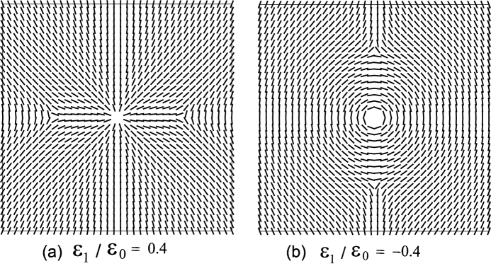
Figure 6: The director field in two dimensions for $\varepsilon_{1}/\varepsilon_{0}=0.4$ in (a) and for $\varepsilon_{1}/\varepsilon_{0}=-0.4$ in (b) around a charged wire at the origin. It tends to be along the $y$ axis (in the vertical direction) far from the origin. The spacing between the adjacent bars is $2\ell_{\rm B}$.

Fig.6 illustrates the deformation of $n$ in two dimensions. We have numerically solved

$${\mbox{\boldmath$n$}}\times\bigg{[}K\nabla^{2}{\mbox{\boldmath$n$}}+\frac{\varepsilon_{1}}{4\pi}({\mbox{\boldmath$E$}}\cdot{\mbox{\boldmath$n$}}){\mbox{\boldmath$E$}}\bigg{]}={\mbox{\boldmath$0$}},$$ (5.25)

under $-\nabla\cdot\stackrel{{\scriptstyle\leftrightarrow}}{{{\varepsilon}}}\cdot\nabla\phi=4\pi\rho$ by assuming ${\mbox{\boldmath$n$}}=(\cos\theta,\sin\theta)$ (or $n_{z}=0$). A charge is placed in the hard-core region $(x^{2}+y^{2})^{1/2}<R$. In three dimensions this is the case of an infinitely long charged wire with radius $R$ and charge density $\sigma$, in which all the quantities depend only on $x$ and $y$. The solution can be characterized by the three normalized quantities, $\varepsilon_{1}/\varepsilon_{0}$, $\sigma^{*}\equiv\sigma/(\varepsilon_{0}K)^{1/2}$, and $R/\ell_{\rm B}$. Here we set $\sigma^{*}=2.4$ and $R/\ell_{\rm B}=2$. We discretize the space into a $200\times 200$ lattice in units of $\ell_{\rm B}$ under the periodic boundary condition in the $x$ direction, so the system width is $L=200\ell_{\rm B}$. The electric potential vanishes at $y=0$ and $L$.

6 Concluding remarks

(i) The Ginzburg-Landau theory in Section 2 generally describes how the electrostatic interactions arise depending on the boundary condition (in the presence or absence of the capacitor plates). It can be used to investigate electric field effects at various kinds of phase transitions in fluids and solids.
(ii) A brief review has been given on the dielectric properties and the electric field effects in near-critical fluids and liquid crystals. The Debye-Kleboth experiment on the critical temperature shift was performed many years ago and they neglected the dipolar interaction in their theoretical interpretation. As regards the nonlinear dielectric constant $\Delta\varepsilon_{\rm eff}$ and the birefringence $\Delta n$, we cannot explain their experimental exponents, $z_{\rm non}\sim 0.4$ and $z_{\rm op}\cong 0.65-0.8$, whereas the common exponent $\nu(1-2\eta)\cong 0.58$ has been predicted for them. To resolve these issues, scattering experiments to check the anisotropic structure factor (3.17) are most needed.
(iii) New predictions have also been made on the critical temperature shift due to electric field, the nonlinear dielectric constant, the ion effects in binary mixtures, and the fluctuation intensities and the form dichroism in liquid crystals. In particular, in near-critical polar mixtures with ions, we have examined charge distributions and potential differences around two-phase interfaces, the critical temperature shift due to ions, and the scattering intensity. The condition for a charge-density-wave phase has been examined for general multivalent ions.
(iv) Effects of oscillating electric field are also worth studying particularly for ionic systems. Appreciable critical anomaly can be seen in the frequency-dependence of the dielectric constant [49]. Large dynamic electric birefringence was observed in polyelectrolyte solutions [51]. By this method we can neglect accumulation of ions at the boundaries (but the Joule heating may not be negligible).
(v) In Section 5 we have examined the deformation of the nematic order around a charged particle. The charge-induced orientation is intensified with decreasing the particle radius $R$ and/or increasing the charge number $Z$. This is in marked contrast to the surface anchoring of a neutral particle [52, 53], which can be achieved for large radius because the penalty of the Frank free energy needs to be small. For charged colloidal suspensions, furthermore, the counterions themselves can induce large deformation of the nematic order (because of their small size) and tend to accumulate near the large particles. These aspects should be examined in future.
(vi) Stronger electric field effects have been observed in polymeric systems than in low-molecular-weight fluids. As such effects, we mention field-induced anisotropy in light scattering from a polymer solution [32], lamellar alignment in diblock copolymers [54], and large dielectric response in a surfactant sponge phase [55].

Acknowledgments

I would like to thank S.J. Rzoska for valuable discussions on the electric field effects in fluids. Thanks are also due to K. Orzechowski for guidance of the ion effects in binary mixtures and for showing Refs.$[41$-$43]$. G.G. Fuller informed me of Ref.[50].

References

- [1] L.D. Landau and E.M. Lifshitz, Electrodynamics of Continuous Media (Pergamon, 1984), Chap II.
- [2] P. Debye and K. Kleboth, J. Chem. Phys., 42, 3155 (1965).
- [3] D. Bedeaux and P. Mazur, Physica 67, 23 (1973).
- [4] G. Stell and J.S. Hoye, Phys. Rev. Lett. 33, 1268 (1974); J.S. Hoye and G. Stell, J. Chem. Phys. 81, 3200 (1984).
- [5] J. Goulon, J.L. Greffe and D.W. Oxtoby, J. Chem. Phys. 70, 4742 (1979).
- [6] J.V. Sengers, D. Bedeaux, P. Mazur and S.C. Greer, Physica, 104A, 573 (1980).
- [7] D. Beaglehole, J. Chem. Phys. 74, 5251 (1981).
- [8] A. Onuki and M. Doi, Europhys. Lett. 17, 63 (1992).
- [9] A. Onuki, Europhys. Lett. 29, 611 (1995).
- [10] G. Zalczer and D. Beysens, J. Chem. Phys. 92, 6747 (1990).
- [11] J. Malecki and J. Zioło, Chem Phys. 35, 187 (1978).
- [12] W. Pyzuk, Chem Phys. 50, 281 (1980); Europhys. Lett. 17, 339 (1992).
- [13] S.J. Rzoska, J. Chrapeć and J. Zioło , Physica A 139, 569 (1980); S.J. Rzoska, A. D. Rzoska, M. Grny and J. Zioło, Phys. Rev. E 52, 6325 (1995).
- [14] S.J. Rzoska, Phys. Rev. E 48, 1136 (1993).
- [15] K. Orzechowski, Physica B 172, 339 (1991); Chem. Phys. 240, 275 (1999).
- [16] W. Pyzuk, H. Majgier-Baranowska, and J. Zioło, Chem Phys. 59, 111 (1981).
- [17] R. Piazza, T. Bellini, V. Degiorgio, R.E. Goldstein, S. Leibler and R. Lipowsky, Phys. Rev. B 38, 7223 (1988).
- [18] T. Bellini and V. Degiorgio, Phys. Rev. B 39, 7263 (1989).
- [19] S.J. Rzoska, V. Degiorgio, T. Bellini and R. Piazza, Phys. Rev. E 49, 3093 (1994).
- [20] P.G. de Gennes and J. Prost, The Physics of Liquid Crystals (Oxford, 1993).
- [21] W. Pyzuk, I. Stomka, J. Chrapeć, S.J. Rzoska, and J. Zioło, Chem Phys. 121, 255 (1988); A. Drozd-Rzoska, Phys. Rev. E 59, 5556 (1999).
- [22] A. Onuki, Phase Transition Dynamics (Cambridge, 2002).
- [23] A. Onuki and K. Kawasaki, Physica A 11, 607 (1982).
- [24] A. Onuki and M. Doi, J. Chem. Phys. 85 1190 ( 1986).
- [25] Y.C. Chou and W.I. Goldburg, Phys. Rev. Lett. 47, 1155 (1981); D. Beysens and M. Gbadamassi, Phys. Rev. Lett. 47, 846 (1981); D. Beysens, R. Gastand and Decrupppe, Phys. Rev. A 30, 1145 (1984).
- [26] N.J. Wagner, G.G. Fuller, and W.B. Russel, J. Chem. Phys. 89, 1580 (1988)
- [27] D. Wirtz, D.E. Werner and G.G. Fuller, J. Chem. Phys. 101, 1679 (1994).
- [28] R. Kretschmer and K. Binder, Phys. Rev. B 20, 1065 (1979).
- [29] B. Groh and S. Dietrich, Phys. Rev. E 53, 2509 (1996); 57, 4535 (1998).
- [30] T. Garel and S. Doniach, Phys. Rev. B 26, 325 (1982).
- [31] Y. Yoshida and A. Ikushima, J. Phys. Soc. Jpn. 45, 1949 (1978).
- [32] D. Wirtz, K. Berend, and G.G. Fuller, Macromolecules 25, 7234 (1992); D. Wirtz and G.G. Fuller, Phys. Rev. Lett. 71, 2236 (1993).
- [33] A. Aharony, Phys. Rev. B 8, 3363 (1973).
- [34] M.E. Fisher and J.S. Langer, Phys. Rev. Lett. 20, 665 (1968).
- [35] G. Zimmerli, R.A. Wilkinson, R.A. Ferrell and M.R. Moldover, Phys. Rev. E 59, 5862 (1999).
- [36] M. Barmartz and F. Zhong, Proceedings of the 2000 NASA/JPL Workshop on Fundamental Physics in Microgravity, Solvang, June 19-21, 2000.
- [37] J.I. Frenkel, Phys. Z. Sowjetunion 8, 675 (1935) [Zh.Eksp.Teor.Fiz. 6, 347 (1936)]; L. Tonks, Phys. Rev. 48 , 562 (1935); G.I. Taylor and A.D. McEwan, J. Fluid Mech. 22, 1 (1965).
- [38] L.P. Gorkov and D.M. Chernikova, Pis’ma Zh. Eksp. Teor. Fiz. 18, 119 (1973) [JETP Lett. 18, 68 (1973)]; M. Wanner and P. Leiderer, Phys. Rev. Lett. 42, 315 (1979); D. Savignac and P. Leiderer, Phys. Rev. Lett. 49, 1869 (1992).
- [39] A. Onuki, Physica A, 217, 38 (1995).
- [40] J.N. Israelachvili, Intermolecular and Surface Forces (Academic, 1985).
- [41] E.L. Eckfeldt and W.W. Lucasse, J. Phys. Chem. 47, 164 (1943).
- [42] B.J. Hales, G.L. Bertrand, and L.G. Hepler, J. Phys. Chem. 70, 3970 (1966).
- [43] J.L. Tveekrem and D.T. Jacobs, Phys. Rev. A 27, 2773 (1983).
- [44] T. Narayanan and A. Kumar, Phys. Rep. 249, 135 (1994); J. Jacobs, A Kumar, M.A. Anisimov, A.A. Povodyrev and J.V. Sengers, Phys. Rev. E 58, 2188 (1998).
- [45] K. Yoshida, M. Misawa, K. Maruyama, M. Imai, and M. Furusaka, J. Chem. Phys. 113, 2343 (2000).
- [46] M. Born, Z. Phys. 1, 45 (1920).
- [47] J.F. Joanny and L. Leibler, J. Phys. (France) 51, 545 (1990); P.M. Chaikin and T.C. Lubensky, Principles of Condensed Matter Physics (Cambridge, 1995).
- [48] V.M. Nabutovskii, N.A. Nemov, and Yu.G. Peisakhovich, Phys. Lett. A, 79, 98 (1980); Sov. Phys. JETP 52, 111 (1980) Zh.Eksp.Teor.Fiz. 79, 2196 (1980); Mol. Phys. 54, 979 (1985).
- [49] K. Orzechowski, private communication and the paper in this conference.
- [50] D. Langevin and M.-A. Bouchiat, J. de Physique C1, 36, 197 (1975).
- [51] U. Krmer and H. Hoffmann, Macromolecules, 24, 256 (1991).
- [52] E. M. Terentjev, Phys. Rev. E 51, 1330 (1995).
- [53] P. Poulin, H. Stark, T. C. Lubensky,snd D. A. Weitz, Science 275 1770 (1997).
- [54] K. Amundson, E. Helfand, X. Quan, S.D. Hudson, and S.D. Smith, Mcromolecules, 27, 6559 (1994); A. Onuki and J. Fukuda, Mcromolecules, 28, 8788 (1995).
- [55] M.E. Cates, P. van der Schoot, and C.-Y.D. Lu, Europhys. Lett. 29, 689 (1995).