Measurement of Two-Qubit States by a Two-Island Single Electron Transistor

Abstract

We solve the master equations of two charged qubits measured by a single-electron transistor (SET) consisted of two islands. We show that in the sequential tunneling regime the SET current can be used for reading out results of quantum calculations and providing evidences of two-qubit entanglement, especially when the interaction between the two qubits is weak.

Quantum information processing in solid state nanostructures has attracted wide spread attention because of the potential scalability of such devices. Within this context, quantum measurement in mesoscopic systems is a crucial issue and is being carefully analyzed both experimentally Nakamura ; Fujisawa ; Wiel ; Aassime and theoretically Gurvitz ; Goan ; Makhlin ; Kane ; Loss ; Korotkov ; Tanamoto ; Miranowicz , so that proper measurements can be designed to extract the maximal amount of information contained in a solid state qubit (or qubits). One prominent example is a single-electron transistor (SET), whose current is particularly sensitive to the charge degrees of freedom through gate potential variations on its central island(s). Indeed, with a radio-frequency SET, electrons can be counted at frequencies up to 100 MHz Aassime , so that if the states of a qubit can be distinguished by charge locations, an SET can be used to measure the qubit states.

Recently, two-qubit coherent evolution and possibly entanglement have been observed in capacitively coupled Cooper pair boxes Pashkin . The realization and detection of two-qubit entanglement are crucial milestones for the study of solid state quantum computing. In this Letter we study a novel scheme for the quantum measurement of two charge qubits ($N\!=\!2$), which can be extended to the detection of moderately larger number of qubits ($N\!>\!2$). Specifically, the target qubits being constantly measured are double dot charge qubits Tanamoto , whose states are the different spatial distributions of the excess electron on the double dot. The quantum detector is a two-island SET ($N\!=\!2$), with each island coupled to a qubit capacitively, as illustrated in Fig. 1. Our objective is to demonstrate the capability of this two-island SET in detecting and differentiating two-qubit quantum states. In particular, we develop a master equation formalism from microscipic Hamiltonian to describe the readout current of the SET in its sequential tunneling regime. Under the condition that the relaxation time of SET current is sufficiently long compared to the period of qubit oscillations, we clarify three major issues regarding the capability of the two-island SET layout: whether the two-qubit eigenstates $\{|00\rangle,|01\rangle,|10\rangle,{\rm and}|11\rangle\}$ can be distinguished; whether entangled states and product states can be distinguished; and whether Zeno effect can be seen in the two qubits.

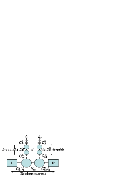
Figure 1: Qubits are capacitively coupled to a two-island SET, which acts as a charge detector. $N(\geq\!2)$ qubits are arranged between source and drain.

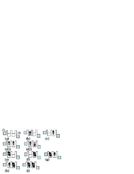
Figure 2: Electronic states in the detector.

The Hamiltonian for the combined two qubits and the two-island SET can be written as follows:

$$H=H_{\rm qb}+H_{\rm set}+H_{\rm int}.$$ (1)

where $H_{\rm qb}$, $H_{\rm set}$, and $H_{\rm int}$ are the Hamiltonians of the two qubits, the SET, and the interaction between the qubits and the SET, respectively. $H_{\rm qb}$ describes the two interacting (left and right, as illustrated in Fig. 1) qubits, each consisted of two tunnel-coupled quantum dots (QDs) and containing one excess charge Tanamoto :

$$H_{\rm qb}\!=\!\sum_{\alpha\!=\!L,R}(\Omega_{\alpha}\sigma_{\alpha x}\!+\!\Delta_{\alpha}\sigma_{\alpha z})\!+\!J\sigma_{Lz}\sigma_{Rz}$$ (2)

where $\Omega_{L}(\Omega_{R}$) and $\Delta_{L}(t)[\Delta_{R}(t)]$ are the inter-QD (but intra-qubit) tunnel coupling and energy difference in the left (right) qubit. Here we use the spin notation such that $\sigma_{\alpha x}\equiv a_{\alpha}^{\dagger}b_{\alpha}+b_{\alpha}^{\dagger}a_{\alpha}$ and $\sigma_{\alpha z}\equiv a_{\alpha}^{\dagger}a_{\alpha}-b_{\alpha}^{\dagger}b_{\alpha}$ ($\alpha=L,R$), where $a_{\alpha}$ and $b_{\alpha}$ are the annihilation operators of an electron in the upper and lower QDs of each qubit. $J$ is a coupling constant between the two qubits, originating from capacitive couplings in the QD system Tanamoto . $|\!\uparrow\rangle$ and $|\!\downarrow\rangle$ refer to the two single-qubit states in which the excess charge is localized in the upper and lower dot, respectively. $\Delta_{\alpha}$ ($\alpha=L,R)$ are bias gate voltages applied on the qubits, which can be used to tune the qubit energy splittings and are used for the manipulation of these charge qubits during quantum calculations Tanamoto . The SET part of the Hamiltonian $H_{\rm set}$ is written as:

$$H_{\rm set}\!=\!\!\!\!\sum_{\alpha\!=L,R}\!\left[\sum_{i_{\alpha},s}E_{i_{\alpha}}c_{i_{\alpha}s}^{\dagger}c_{i_{\alpha}s}\!+\!\sum_{s}E_{d_{\alpha}s}d_{\alpha s}^{\dagger}d_{\alpha s}\!+\!U_{\alpha}n_{\alpha\uparrow}n_{\alpha\downarrow}\right]$$ (3)

$$+\sum_{\alpha\!=\!{\small L,R}}\sum_{i_{\alpha},s}\!V_{\alpha s}\left(c_{i_{\alpha}s}^{\dagger}d_{\alpha s}\!+\!d_{\alpha s}^{\dagger}c_{i_{\alpha}s}\right)$$

$$+\sum_{s}V_{Ms}\left(d_{Ls}^{\dagger}d_{Rs}\!+\!d_{Rs}^{\dagger}d_{Ls}\right).$$

Here $c_{i_{L}s}$($c_{i_{R}s}$) is the annihilation operator of an electron in $i_{L}$th ($i_{R}$th) level ($i_{L}(i_{R})=1,...,n)$, in the left(right) electrode, $d_{Ls}$($d_{Rs}$) is the electron annihilation operator of the left (right) SET island, $s\in\{\uparrow,\downarrow\}$ is the electron spin, and $n_{\alpha s}\equiv d_{\alpha s}^{\dagger}d_{\alpha s}$ is the number of electron on each island. Here we assume only one energy level on each island. $V_{Ls}$($V_{Rs}$) and $V_{Ms}$ are the tunneling strength of electrons between left (right) electrode and the left (right) island and that between the two islands. $U_{L}(U_{R})$ is the on-site Coulomb energy of double occupancy in the left (right) island. Finally, the interaction between the qubits and the SET, described by $H_{\rm int}$, are capacitive couplings between the qubits and the two SET islands:

$$H_{\rm int}=\sum_{s}\left(E_{\rm int}^{L}d_{Ls}^{\dagger}d_{Ls}\sigma_{Lz}\!+\!E_{\rm int}^{R}d_{Rs}^{\dagger}d_{Rs}\sigma_{Rz}\right).$$ (4)

Consequently, the energy level of an SET island is raised by $E_{\rm int}^{\alpha}\!\sim eC_{\rm int}^{\alpha}C_{\rm A}^{\alpha}/C_{\rm S}^{\alpha}/(C_{\rm A}^{\alpha}C_{\rm int}^{\alpha}\!+\!C_{\rm B}^{\alpha}[C_{\rm A}^{\alpha}\!+\!C_{\rm int}^{\alpha}])$ if the charge in the corresponding qubit is located in the lower QD Makhlin . The electronic states of the qubits also influence the tunneling rates $\Gamma^{\alpha}(E)\!=\!2\pi\rho_{\alpha}(E)|V_{\alpha}(E)|^{2}$ ($\rho_{\alpha}$ are densities of states of the electrodes). If we define $\{|A\rangle\!\equiv\!|\!\downarrow\downarrow\rangle$, $|B\rangle\!\equiv\!|\!\downarrow\uparrow\rangle$, $|C\rangle\!\equiv\!|\!\uparrow\downarrow\rangle$, $|D\rangle\!\equiv\!|\!\uparrow\uparrow\rangle\}$, the tunneling rates have the relations; $\Gamma^{L}_{A}\!=\!\Gamma^{L}_{B}\!<\!\Gamma^{L}_{C}\!=\!\Gamma^{L}_{D}$ and $\Gamma^{R}_{A}\!=\!\Gamma^{R}_{C}\!<\!\Gamma^{R}_{B}\!=\!\Gamma^{R}_{D}$.

Now we can construct the equations of the qubits-SET density matrix elements governed by the above-mentioned Hamiltonian at $T\!=\!0$, following the procedure developed by Gurvitz Gurvitz . The possible electronic states in the detector are shown in Fig. 2. The method is applicable as long as the energy-levels of the islands is inside the chemical potential $\mu_{L}$ of the left electrode and $\mu_{R}$ of the right electrode, and the tunneling rates are much smaller than the difference $\mu_{L}-$ $\mu_{R}$, i.e. $\mu_{L}-\mu_{R}\gg\{\Gamma^{L},\Gamma^{R},V_{M}$} Stoof . We consider the following two transport processes separately. The first case is when the double-occupied states are inside the range of $\mu_{L}$ and $\mu_{R}$ and all electronic states in Fig.2 take part in the tunneling (finite $U$ model). The second case is when double occupancy of electrons [(e)-(i)] is prohibited (infinite $U$ model). Experimentally, these two cases are interchangeable by tuning applied island gate voltages Double .

The wave function $|\Psi(t)\rangle$ of the qubits-SET system can be expanded over the electronic states of the qubits and the island states of the SET shown in Fig. 2. Assuming that there is no magnetic field and the tunneling is independent of spin, after a lengthy calculation, we obtain 352 equations for density matrix elements $\rho_{u_{1}u_{2}}^{z_{1}z_{2}}(t)$ ($u_{1},u_{2}$ indicate quantum states of the detector (Fig. 2) and $z_{1},z_{2}=A,B,C,D$ are those of the qubits) as num_of_eq :

$$\dot{\rho}_{aa}^{AA}\! = \!-2\Gamma^{L}\rho_{aa}^{AA}\!-\!i\Omega_{R}(\rho_{aa}^{BA}\!-\!\rho_{aa}^{AB})\!-\!i\Omega_{L}(\rho_{aa}^{CA}\!-\!\rho_{aa}^{AC})$$

$$+\Gamma^{R}(\rho_{cc\uparrow}^{AA}\!+\!\rho_{cc\downarrow}^{AA}),$$

$$\dot{\rho}_{aa}^{AB}\! = \!(i[\!-\!J_{A}\!+\!J_{B}]\!-\!2\Gamma^{L})\rho_{aa}^{AB}\!-i\Omega_{R}(\rho_{aa}^{BB}\!-\!\rho_{aa}^{AA})$$

$$\!-\!i\Omega_{L}(\rho_{aa}^{CB}\!-\!\rho_{aa}^{AD})\!+\!\Gamma^{R}(\rho_{cc\uparrow}^{AB}\!+\!\rho_{cc\downarrow}^{AB}),$$

$$......$$

$$\dot{\rho}_{ii}^{CD}\! = \!\!2(i[\!-\!E_{d_{L}}^{C}\!-\!E_{d_{R}}^{C}\!+\!E_{d_{L}}^{D}\!+\!E_{d_{R}}^{D}\!-\!J_{C}\!+\!J_{D}]\!-\!\Gamma^{R^{\prime}})\rho_{ii}^{CD}$$ (5)

$$-i\Omega_{R}(\rho_{ii}^{DD}\!-\!\rho_{ii}^{CC})\!-\!i\Omega_{L}(\rho_{ii}^{AD}\!-\!\rho_{ii}^{CB})$$

$$+\Gamma^{L^{\prime}}(\rho_{hh\uparrow}^{CD}\!+\!\rho_{hh\downarrow}^{CD}),$$

where $J_{A}=\Delta_{L}\!+\!\Delta_{R}\!+\!J$, $J_{B}=\Delta_{L}\!-\!\Delta_{R}\!-\!J$, $J_{C}=-\Delta_{L}\!+\!\Delta_{R}\!-\!J$, $J_{D}=-\Delta_{L}\!-\!\Delta_{R}\!+\!J$, $E_{d_{L}}^{A}=E_{d_{L}}^{B}=E_{d_{L}}\!+\!E_{\rm int}^{L}$, $E_{d_{L}}^{C}=E_{d_{L}}^{D}=E_{d_{L}}\!-\!E_{\rm int}^{L}$, $E_{d_{R}}^{A}=E_{d_{R}}^{C}=E_{d_{R}}\!+\!E_{\rm int}^{R}$, $E_{d_{R}}^{B}=E_{d_{R}}^{D}=E_{d_{R}}\!-\!E_{\rm int}^{R}$. $\Gamma^{\alpha^{\prime}}\!=\!0$ in infinite $U$ model and $\Gamma^{\alpha^{\prime}}\!=\!\Gamma^{\alpha}$ in finite $U$ model. The readout current $I(t)\!=\!e\dot{N}_{R}(t)$ can then be written as Gurvitz

$$I(t)\! = \!\!\!\!\!\!\!\!\!\!\sum_{z=A,B,C,D}\!\!\!\!\!\!\!\!\!e\{\Gamma^{R}[\rho_{cc\uparrow}^{zz}\!+\!\rho_{cc\downarrow}^{zz}\!+\!\rho_{d_{\uparrow\uparrow}d_{\uparrow\uparrow}}^{zz}\!\!\!+\!\rho_{d_{\downarrow\uparrow}d_{\downarrow\uparrow}}^{zz}\!\!\!+\!\rho_{d_{\uparrow\downarrow}d_{\uparrow\downarrow}}^{zz}\!\!\!+\!\rho_{d_{\downarrow\downarrow}d_{\downarrow\downarrow}}^{zz}\!\!$$ (6)

$$\!+\! \!2\rho_{ff}^{zz}\!+\!\rho_{gg\uparrow}^{zz}\!+\!\rho_{gg\downarrow}^{zz}\!\!+\!\!2(\rho_{hh\uparrow}^{zz}\!+\!\rho_{hh\downarrow}^{zz})]\!+\!2\Gamma^{R^{\prime}}\!\rho_{ii}^{zz}\}.$$

For simplicity we consider two identical qubits, with $E_{d_{L}}\!=\!E_{d_{R}}$ and $E_{\rm int}\equiv E_{\rm int}^{L}\!=\!E_{\rm int}^{R}$.

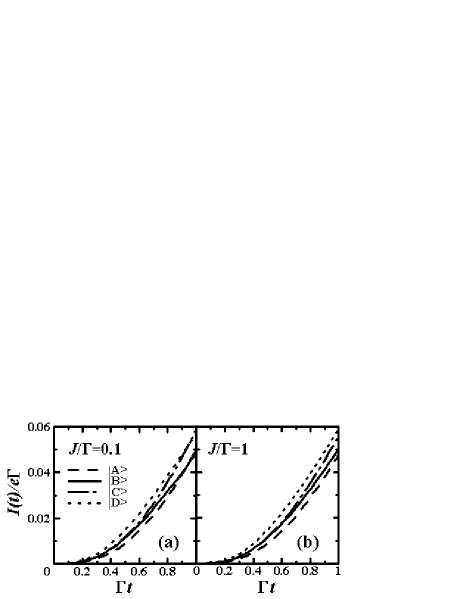
Figure 3: Time dependent readout current characteristics of the infinite $U$ model for $|A\rangle=|\downarrow\downarrow\rangle$, $|B\rangle=|\downarrow\uparrow\rangle$, $|C\rangle=|\uparrow\downarrow\rangle$, $|D\rangle=|\uparrow\uparrow\rangle$ as initial states ($t=0$), where $\Omega_{L}=\Omega_{R}=0.75\Gamma$, $V_{M}=0.5\Gamma$, $E_{\rm int}^{L}=E_{\rm int}^{R}=0.2\Gamma$, $\Gamma^{L}_{A}\!=\!\Gamma^{L}_{B}\!=\Gamma^{R}_{A}\!=\!\Gamma^{R}_{C}=0.8\Gamma$, $\Gamma^{L}_{C}\!=\!\Gamma^{L}_{D}=\Gamma^{R}_{B}\!=\!\Gamma^{R}_{D}=1.2\Gamma$. (a) $J=0.1\Gamma$, (b) $J=\Gamma$.

We monitor the onset of the readout current to extract information of the qubit states. The current begins to flow at $t=0$ and after a transient region saturates to a steady state value. In the meantime, the qubits oscillate with frequencies $\sqrt{\Omega_{\alpha}^{2}+\Delta_{\alpha}^{2}}$. The interaction with the dissipative current degrades the coherent oscillations and makes the charge distribution uniform in the qubits at $t\rightarrow\infty$. Conversely, in the absence of the qubits, the current saturates around $t\sim\Gamma^{-1}$ where $\Gamma\!\equiv\!\Gamma^{L}\Gamma^{R}/(\Gamma^{L}\!+\!\Gamma^{R})$, while the qubit charge oscillations modify the SET current through an effective gate potential on the islands. Figure 3 shows the time-dependent current characteristics of the infinite $U$ model near $t\sim 0$. At small $t$ state $|A\rangle$ suppresses the current the most while state $|D\rangle$ the least. The measurement time $t_{m}$ that is required to resolve the states of qubits is estimated as $t_{\rm m}^{-1}\!\sim\!{\rm min}\{E_{\rm int},\Gamma_{A}^{L}\!-\!\Gamma_{D}^{L}\}$ ($\sim 0.5^{-1}\Gamma$ in Fig. 3). The relative magnitude of the current changes after the coherent motions of qubits ($t>1/\Omega_{\alpha}$). Thus the SET current can be used to distinguish the four product states during $t_{\rm m}<t<1/\Omega_{\alpha}$. If the coherent oscillation of the qubits remains after $t>\Gamma^{-1}$, as in the present model phonon , we can discuss the quantum states of qubits using the steady current formula ($t\rightarrow\infty$) through the SET without the qubits Gurvitz :

$$I_{\rm set}=\frac{e\Gamma V_{M}^{2}}{\epsilon_{d}^{2}\Gamma/(\Gamma^{L}\!+\!\Gamma^{R})\!+\!V_{M}^{2}\!+\!\Gamma^{L}\Gamma^{R}/4},$$ (7)

where $\epsilon_{d}\equiv E_{d_{L}}-E_{d_{R}}$ is the energy difference of the two islands. If $V_{M}\gg{\Gamma,\epsilon_{d},\Omega_{\alpha}}$, the coupling between the two islands is strong and the current mainly reflects the bonding-antibonding state in the detector, which is not suitable for qubit measurements. We thus focus on the regime of $V_{M}<\Omega_{\alpha},\Gamma$. Since $E_{d_{L}}^{A}\!-\!E_{d_{R}}^{A}\!=\!E_{d_{L}}^{D}\!-\!E_{d_{R}}^{D}\!=\!0$ and $E_{d_{L}}^{B}\!-\!E_{d_{R}}^{B}\!=\!E_{d_{R}}^{C}\!-\!E_{d_{L}}^{C}\!=\!2E_{\rm int}$, the different effects between $|A\rangle$ and $|D\rangle$ and that between $|B\rangle$ and $|C\rangle$ come from the differences in the tunneling rates. Moreover, the difference of $|A\rangle$ and $|D\rangle$ from $|B\rangle$ and $|C\rangle$ becomes obvious in the $E_{\rm int}>V_{M}$ region. Thus we call $E_{\rm int}>V_{M}$ strong measurement regime, where the four product states can be distinguished, in contrast to the weak measurement regime of $E_{\rm int}<V_{M}$.

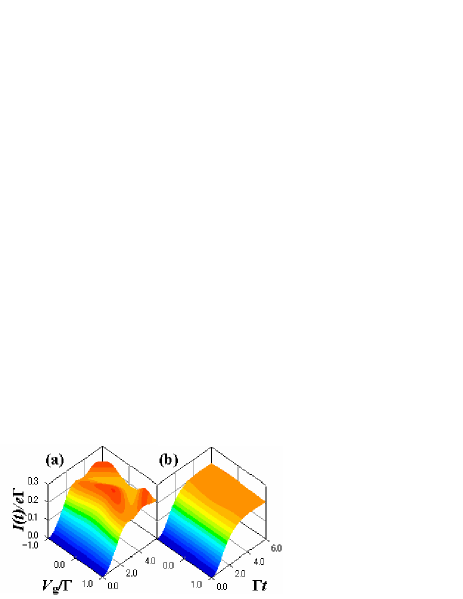
Figure 4: Time dependent readout current characteristics starting from :(a) $|B\rangle$, (b) singlet state in the infinite $U$ model for weak measurement case ($E_{\rm int}\!=\!0.2\Gamma<\!V_{M}\!=\!0.5\Gamma$) as a function of $V_{\rm g}\!=\!V_{\rm g}^{L}\!=\!V_{\rm g}^{R}$. Parameters are the same as those in Fig.3.

We can distinguish the current of pure entangled states and that of pure product states by changing bias voltages $V_{g}^{\alpha}=\Delta_{\alpha}$ in the regime of $J/\Gamma\ll 1$, where the current depends on the change of qubit oscillation frequency ($\sim\sqrt{\Omega_{\alpha}^{2}+\Delta_{\alpha}^{2}}$). Figure 4(a) shows the current corresponding to the qubit $|B\rangle$ state in the weak measurement regime of the infinite $U$ model. We also obtained similar results for the other product states $|A\rangle$, $|C\rangle$, and $|D\rangle$. In contrast, the readout current for a two-qubit entangled state is more uniform compared with the product states as entangled states generally have less distinct charge distributions. For example, the density matrix elements for a singlet state $(|\!\!\uparrow\downarrow\rangle\!-\!|\!\!\downarrow\uparrow\rangle)/\sqrt{2}=(|C\rangle\!-\!|B\rangle)/\sqrt{2}$ of two free qubits ($H_{\rm int}=0$) satisfy $\dot{\rho}^{BB}\!+\!\dot{\rho}^{CC}\!-\!\dot{\rho}^{BC}\!-\!\dot{\rho}^{CB}\!=0$ ($\Delta_{L}=\Delta_{R}$), which suggests that entangled states such as the singlet state are less effective in influencing the readout current. We believe this ineffectiveness is related to the fact that logical states encoded in entangled states are less susceptible to environmental decoherence Palma . Indeed, the readout current of this entangled state is found to be uniform as shown in Fig. 4(b). We obtained similar results for the other Bell states, and there is no significant difference between the infinite $U$ model and the finite $U$ model in the weak measurement regime.

In the strong measurement regime ($E_{\rm int}>V_{M}$), the current is more sensitive to the charge distributions in the qubits, and there are differences between the infinite $U$ model and finite $U$ model. We can distinguish the four products more easily through the SET current, as shown in Fig. 5(a)-(d). However, currents for the entangled states in the infinite $U$ model show several similar peaks that reflect the qubit oscillations and cannot be easily distinguished from the product states. On the other hand, the finite $U$ model shows distinct uniform structure compared with the current of the product states [Fig. 5(e) and (f)]. This shows that, in the finite $U$ model, redistribution of the electrons through the two islands of the detector is energetically favorable under the rather uniform electric field generated by the entangled qubits. Figure 6(a) shows that the concurrence (a measure of entanglement Wootters derived from reduced density matrix of two qubits after tracing over the detector components) of the two qubits disappears quickly in the cases of strong measurement. While the coherence quickly degrades, we can see the emergence of the Zeno effect, in which a continuous measurement slows down transitions between quantum states due to the collapse of the wavefunctions into observed states Gurvitz ; Korotkov . For instance, Fig. 6 (b) shows that, as $E_{\rm int}$ increases, the oscillations of density matrix elements of the qubits (e.g. $\rho^{DD}$) are delayed, which is a clear evidence of the slowdown described by the Zeno effect in the two qubits.

Our numerical results above are applicable to a wide range of pure product and entangled states. For example, in the entangled states $\cos\theta|\!\uparrow\downarrow\rangle+e^{i\varphi}\sin\theta|\!\uparrow\downarrow\nobreak\rangle$, we found that the uniformity of the readout current holds approximately up to $|\theta\pm\pi/4|,|\varphi|<\pi/12$. The pure entangled states are more robust beyond the spatial distribution of the wave functions. Although the product states $\!\prod_{\alpha\!=\!L,R}[\cos(\frac{\theta_{\alpha}}{2}){\rm e}^{-i\frac{\varphi_{\alpha}}{2}}|\uparrow\rangle_{\alpha}\!+\!\sin(\frac{\theta_{\alpha}}{2}){\rm e}^{i\frac{\varphi_{\alpha}}{2}}|\downarrow\rangle_{\alpha}]$ seem to have similarly uniform wave functions when $\theta_{L}=\pm\theta_{R}$ and $\varphi_{L}=\pm\varphi_{R}=0,\pi$ (compared to the entangled states mentioned above), the corresponding currents reflect the coherent oscillations of the qubits when the gate bias changes between $V_{g}^{L}=V_{g}^{R}$ and $V_{g}^{L}=-V_{g}^{R}$.

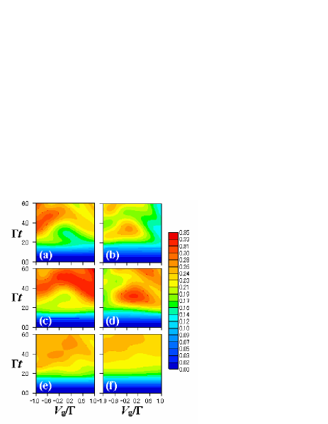
Figure 5: Time dependent readout current characteristics in the finite $U$ model ($U\!=\!2\Gamma$)for strong measurement case ($E_{\rm int}\!=\!0.8\Gamma>\!V_{M}\!=\!0.5\Gamma$) as a function of $V_{\rm g}\!=\!V_{\rm g}^{L}\!=\!V_{\rm g}^{R}$. The initial states are (a) $|A\rangle$, (b) $|B\rangle$,(c) $|C\rangle$,(d) $|D\rangle$, (e) triplet state, (f) singlet state. Parameters other than $E_{\rm int}$ are the same as those in Fig.3.

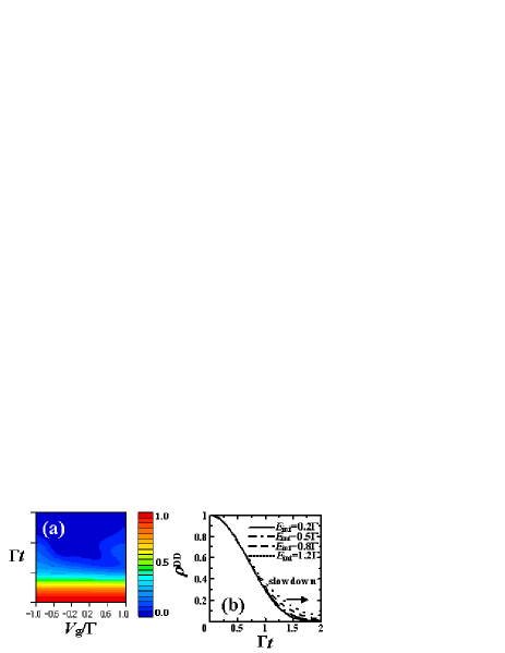
Figure 6: (a) The concurrence of the singlet state. (b) Example of Zeno effect: oscillation of $\rho^{DD}(t)$ is delayed, where the initial state is $|D\rangle$ state ($\rho^{DD}(0)\!=\!1$). Similar effects can be seen in other initial states. Parameters are the same as those in Fig.5.

Since the detection scheme discussed here is based on measuring small current differences in the transient regime, it is important to analyze whether the present day technology can achieve the necessary sensitivity. The state of the art technology allows the measurement of 1 pA current with dynamics in the GHz frequency range with repeated measurement techniques Nakamura ; Fujisawa ; Gardelis . According to our Figs. 3-5, our scheme requires measuring a 0.1 pA current that changes in the nanosecond time scale (assuming a $\Gamma$ in the order of 100 MHz, a reasonable figure because $E_{\rm int}$ would be in the order of 100 MHz if all capacitances are 100 aF), which is at the edge of the current measurement technology. Thus, with a similar design of repeated measurement Nakamura ; Fujisawa ; Gardelis , our detection scheme should be experimentally feasible in the near future.

In conclusion, we have solved master equations and described various time-dependent measurement processes of two charge qubits. The current through the two-island SET is shown to be an effective means to measure results of quantum calculations and entangled states.

We acknowledge discussions with N. Fukushima, S. Fujita, and M. Ueda.

References

(1)
Y. Nakamura et al., Phys. Rev. Lett. 88 047901 (2002).
(2)
T. Fujisawa et al., Phys. Rev. Lett. 88, 236802 (2002).
Phys. Rev. B 63 081304 (2001).
(3)
W. G. van der Wiel et al., Rev. Mod. Phys. 75 1 (2003).
(4)
A. Aassime et al., Phys. Rev. Lett. 86, 3376 (2001).
Schoelkopf et al., Scicence 280, 1238 (1998).
(5)
S. A. Gurvitz and Ya. S. Prager, Phys. Rev. B 53, 15932 (1996).
B. Elattari and S. A. Gurvitz, Phys. Rev. Lett. 84, 2047 (2000).
(6)
H. S. Goan, et al.
Phys. Rev. B 63, 125326 (2001).
(7)
Y. Makhlin et al.,
Rev. Mod. Phys. 73, 357 (2001).
(8)
B. E. Kane et al.,
Phys. Rev. B 61, 2961 (2000).
(9)
D. Loss and E.V. Sukhorukov, Phys. Rev. Lett. 84, 1035 (2000).
(10)
A.N. Korotkov, Phys. Rev. B 60, 5737 (1999);
Phys. Rev. A 65, 052304 (2002).
(11)
T. Tanamoto, Phys. Rev. A 64, 062306 (2001); ibid61, 022305 (2000).
(12)
A. Miranowicz et al., Phys. Rev. A 65 062321 (2002);
Y. Liu et al.,
Phys. Rev. A 65, 042326 (2002).
(13) Yu.A. Pashkin et al.,
Nature 421, 823 (2003).
(14)
T. H. Stoof and Yu. V. Nazarov, Phys. Rev. B 53 1050 (1996).
(15) One limitation of the present formulation is that we cannot
treat the boundary region where the energy of a double occupied island equals
the Fermi energy of an electrode.
(16) We included , , , , ,
, ,
, , , ,
, ,
, , where each
has real and imaginary parts.
(17)
We ignore other origins of decoherence, such as phonons, or trapped charges
that
generate the fluctuations.
(18) G.M. Palma et al., Proc. R. Soc. Lond. 452, 567
(1996); P. Zanardi, Phys. Rev. A 57, 3276 (1998); D. Lidar
et al., Phys. Rev. Lett. 81, 2594 (1998).
(19)
W. K. Wootters, Phys. Rev. Lett. 80, 2245 (1998).
(20)
S. Gardelis et al., Phys. Rev. B 67, 073302 (2003)