Comment on “Frustrating interactions and broadened magnetic interactions in the edge–sharing CuO₂ chains in La₅Ca₉Cu₂₄O₄₁”

Abstract

Using Monte Carlo techniques, we show that the two–dimensional anisotropic Heisenberg model reproducing nicely inelastic neutron scattering measurements on La₅Ca₉Cu₂₄O₄₁ (Matsuda et al. [Phys. Rev. B 68, 060406(R) (2003)]) seems to be insufficient to describe correctly measurements on thermodynamic quantities like the magnetization or the susceptibility. Possible reasons for the discrepancy are suggested.

Recently, Matsuda et al.mat reported results of careful inelastic neutron scattering experiments on La₅Ca₉Cu₂₄O₄₁. From standard spinwave analysis, it is concluded that the experimental data can be well reproduced by a two–dimensional anisotropic spin-1/2 Heisenberg model with antiferromagnetic nearest–neighbor interactions, $J_{c1}$ (= 0.2meV), and ferromagnetic next–nearest–neighbor couplings, $J_{c2}$ ($=-0.18$meV), between the Cu ions in the CuO₂ chains, as well as antiferromagnetic couplings $J_{ac1}$ (= 0.681meV) and $J_{ac2}$ ($=0.5J_{ac1}=0.3405$meV) between nearest and next–nearest neighboring Cu ions in adjacent chains, respectively (see Fig. 1 in Ref. mat, ). The uniaxial anisotropy of the spins along the $b$ axis is written in the form of a single–ion interaction $D$ (= $-0.211$meV), summing over the anisotropy contributions of the different couplings.

This model reproduces the measured dispersion relations along the CuO₂ chains, i.e. along the $c$ axis, and perpendicular to these chains, along the $a$ axis. It is supposed to describe, at low temperatures, the long–range ferromagnetic order in the chains and an antiferromagnetic order perpendicular to the chains.

We performed Monte Carlo simulations on the model in its classical limit with unit vectors as the spins, where the uniaxial anisotropy along the $b$ axis is described either by a single–ion anisotropy,mat $D\sum(S_{j}^{z})^{2}$, or by anisotropic exchange interactions distributing the total anisotropy in various ways among the different couplings. We used exactly the interaction strengths determined in Ref. mat, . To compare the simulational data to previous measurements amm on the magnetization and specific heat of La₅Ca₉Cu₂₄O₄₁, we included external fields $H_{b,c}$ along the $b$ and $c$ axes, and we recorded especially sublattice magnetizations, the total magnetization, the susceptibility, and the specific heat. We took care that reliable equilibrium data were obtained, using at least $5\times 10^{5}$ Monte Carlo steps per spin in each run. We studied finite–size effects, simulating square lattices with the linear dimension ranging from 10 to 100. The square lattice is constructed in such a way that its principal axes are given by the two directions along which $J_{ac1}$ acts between a reference site and the two sites in one of the adjacent chains. Thence the relatively strong coupling $J_{ac1}$ connects nearest–neighbor spins on that lattice, and the CuO₂ chains run diagonally through the lattice. This geometry shows most directly the relation of the model by Matsuda et al. to much studied anisotropic Heisenberg models with nearest–neighbor interactions on square lattices.

Our main findings may be summarized as follows:

(i) For vanishing field and at low temperatures, one obtains, indeed, antiferromagnetic order, i.e. the model describes a ferromagnetic ordering of the spins along the CuO₂ chains and an antiferromagnetic ordering perpendicular to the chains, due to the fairly strong antiferromagnetic couplings $J_{ac1}$ and $J_{ac2}$. The frustrated intrachain couplings $J_{c1}$ and $J_{c2}$, tending to compensate each other, play only a minor role, connecting next–nearest and more distant spins on the square lattice. The transition from the antiferromagnetic to the paramagnetic phase occurs at about $T_{N}=11.5\pm 0.5$K (shifting to somewhat lower temperatures when assigning the uniaxial anisotropy mainly to the intrachain couplings). This apparent agreement with the experimentally observed transition temperature of $10.5$K (Ref. mat, ) resp. $9.7$K (Ref. amm, ) is, however, misleading. Quantum fluctuations are known to reduce the transition temperature in closely related two–dimensional anisotropic spin-1/2 antiferromagnetic quantum Heisenberg models by a factor of about 1.5 in the extreme Ising limit, as compared to $T_{N}$ in the corresponding classical models with unit vectors; for weaker anisotropy the factor tends to increase.cuc ; ser Therefore we conclude that the transition temperature of the anisotropic Heisenberg model mat is expected to be too low compared to the measured $T_{N}$.

(ii) Well above the transition temperature, say, at $1.5\,T_{N}<T<3.0\,T_{N}$, the ratio $r$ of the static susceptibilities (defined by the magnetizations divided by the magnetic fields) along the $b$ and $c$ axes, resp., is found to be almost independent of temperature, both in experiments amm and in the simulations, see Fig. 1. For the anisotropic Heisenberg model, we find that the ratio is also largely independent of the strength of the field (considering fields smaller than the spin–flop field at zero temperature, $H_{b}^{\text{sf}}$= 1.81meV), with $r\approx 1.02$ (approaching one at higher temperatures). The measured ratio is appreciably larger, $r\approx 1.3$, see Fig. 1 in Ref. amm, . This discrepancy may be, however, misleading because the ratio $r$ obtained in the simulations has to be multiplied by the ratio of the squares of the corresponding $g$–factors, $(g_{b}/g_{c})^{2}$, for a correct comparison with the experiments.klin ; mat2 Indeed, the $g$–factor is anisotropic, with $g_{b}/g_{c}\approx 1.14$ for this material.klin ; exp Thence the simulational findings for the ratio $r$ of the magnetizations in differently oriented fields on the anisotropic Heisenberg model with a rather weak anisotropy seems to be consistent with the pertinent experiments.

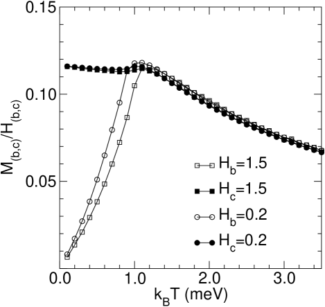
Figure 1: Total magnetization $M_{(b,c)}$ divided by the strength of the differently oriented fields $H_{(b,c)}$ as a function of temperature as obtained from Monte Carlo simulations of the classical version of the Hamiltonian by Matsuda et al. with a single ion anisotropy, Ref. mat, , for a system with 60 $\times$ 60 spins. Note that $H_{(b,c)}$ is expressed in units of meV.

(iii) Applying the field along the $b$ axis, we evaluated the susceptibility $\chi_{b}=\partial M_{b}/\partial H_{b}$ at temperatures below $T_{N}$. Typically, at constant temperature, $\chi_{b}$ displays as a function of $H_{b}$ a strong, delta–like peak at $H_{b}^{\text{sf}}$, signalling the transition from the antiferromagnetic to the spin–flop phase and, at a larger field, $H_{b}^{\text{pm}}$, an additional weak maximum indicating the transition from the spin–flop phase to the paramagnetic phase, see Fig. 2. The spin–flop field $H_{b}^{\text{sf}}$ is nearly independent of temperature below about $0.7\,T_{N}$, decreasing then rather sharply to zero as $T$ approaches $T_{N}$. The upper transition field, $H_{b}^{\text{pm}}$, decreases quite strongly with increasing temperature already at low temperatures. These findings on the anisotropic Heisenberg model are in marked contrast with the observed behavior amm ; klin of $\chi_{b}$ for La₅Ca₉Cu₂₄O₄₁. Experimentally, one also obtains two anomalies in $\chi_{b}$, but a sharp, cusp–like singularity with a rather low maximal height at a small field followed by a broad and higher maximum at larger fields. The location of the upper characteristic field depends, below $T_{N}$, only weakly on temperature. At the lower characteristic field the breakdown of antiferromagnetic order is observed in neutron scattering experiments;klin this field goes to zero as one approaches $T_{N}$. Experimentally, there seems to be no evidence for a transition from the antiferromagnetic phase to a spin–flop phase at the lower characteristic field. The origin and nature of that transition has still to be clarified. At any rate, the results on $\chi_{b}$ for the anisotropic Heisenberg model deviate clearly from the measured behavior.

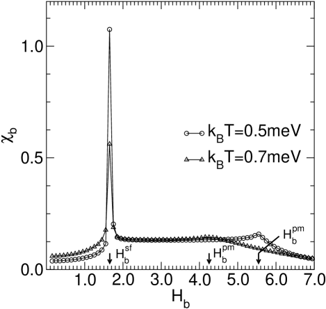
Figure 2: Susceptibility $\chi_{b}=\partial M_{b}/\partial H_{b}$ at $k_{B}T=$ 0.5meV and 0.7meV as determined in simulations of the classical version of the Hamiltonian by Matsuda et al. for a system with 60 $\times$ 60 spins.

From the comparison between the thermodynamic measurements amm ; klin on La₅Ca₉Cu₂₄O₄₁ and the simulational data on the classical version of the model suggested in Ref. mat, , it follows that the model, describing nicely the dispersion relations, seems to be incomplete, missing important ingredients of the real material. Perhaps, as already indicated before,mat the holes induced by the Ca ions may play an important role. A first, simplified modelling of that aspect in the framework of an Ising model has been proposed recently. sel ; hol Furthermore, the couplings of spins in neighboring $ac$–planes may be relevant. Of course, extending the model of Matsuda et al.mat to three dimensions is not expected to resolve the discrepancy about the presence of the spin–flop phase. Finally, structural distortions in La₅Ca₉Cu₂₄O₄₁ may even call for a description going beyond pure spin models.

- (1) M. Matsuda, K. Kakurai, J. E. Lorenzo, L. P. Regnault, A. Hiess, and G. Shirane, Phys. Rev. B 68, 060406(R) (2003).
- (2) U. Ammerahl, B. Büchner, C. Kerpen, R. Gross, and A. Revcolevschi, Phys. Rev. B 62, R3592 (2000).
- (3) A. Cuccoli, T. Roscilde, V. Tognetti, R. Vaia, and P. Verrucchi, Phys. Rev. B 67, 104414 (2003).
- (4) P. A. Serena, N. Garcia, and A. Levanyuk, Phys. Rev. B 47, 5027 (1993).
- (5) R. Klingeler, PhD thesis, RWTH Aachen (2003).
- (6) M. Matsuda, private communication.
- (7) V. Kataev, K.-Y. Choi, M. Grüninger, U. Ammerahl, B. Büchner, A. Freimuth, and A. Revcolevschi, Phys. Rev Lett. 86, 2882 (2002).
- (8) W. Selke, V. L. Pokrovsky, B. Büchner, and T. Kroll, Eur. Phys. J. B 30, 83 (2002).
- (9) M. Holtschneider and W. Selke, Phys. Rev. E 68, 026120 (2003).