Quantum phase transition in a two-channel-Kondo quantum dot device

Abstract

We develop a theory of electron transport in a double quantum dot device recently proposed in Ref. OGG, for the observation of the two-channel Kondo effect. Our theory provides a strategy for tuning the device to the non-Fermi-liquid fixed point, which is a quantum critical point in the space of device parameters. We explore the corresponding quantum phase transition, and make explicit predictions for behavior of the differential conductance in the vicinity of the quantum critical point.

I Introduction

The magnetic screening of a localized spin by spins of itinerant electrons PWA_book leads to the Kondo effect – an anomaly in low-temperature conduction properties. This screening becomes effective below some characteristic temperature, the Kondo temperature $T_{K}$. Above $T_{K}$ electrons are weakly scattered by the magnetic impurity, but below $T_{K}$ the scattering becomes strong. In the simplest Kondo systems, only one electron mode (the $s$-wave mode, say) participates in the screening of a localized spin with $S=1/2$. In this case, the low-temperature electronic properties are adequately described by Fermi liquid theory Nozieres , and the thermodynamic and transport characteristics are analytical functions of $T/T_{K}$. In more complicated systems (such as, e.g., paramagnetic metals) many electron modes may participate in screening of an $S=1/2$ localized moment LM . The peculiarities of such a ”multichannel” Kondo model were long recognized LM ; NB . At the same time it was understood that even a small deviation from symmetry between channels leads at low temperatures to the Kondo screening by just one channel, the one for which the exchange integral with the impurity is the largest NB .

The peculiarity of a symmetric multichannel Kondo problem is in its non-Fermi-liquid (NFL) behavior at low temperatures NB . The low-temperature asymptotes of the thermodynamic and transport characteristics display power-law behavior with fractional values of the exponents. A complete temperature dependence of the thermodynamic characteristics (such as the local spin susceptibility) is known now from the exact Bethe-ansatz solution of the Kondo problem Bethe ; AJ . Details of the low-temperature electron scattering problem were also understood in the framework of conformal field theory Tsvelik ; AL .

Experimental observation of the non-Fermi-liquid behavior in a Kondo system, however, is difficult because the channel symmetry is not “protected” – in general, there are no conservation laws prescribing such a symmetry. This has lead to various propositions to observe such a behavior in systems where the role of spin is taken over by another degree of freedom, while the “real” spin labels the channels, making the channel symmetry robust. One such idea deals with an atomic defect which occupies two equivalent lattice sites, thus forming a pseudospin CZ . However, the equivalence of sites is not a protected symmetry; its violation Aleiner , equivalent to a “Zeeman splitting” of the pseudospin states, destroys the Kondo effect.

Another object which under certain conditions can be described by the two-channel Kondo model (2CK) model, is a large quantum dot, or a metallic island connected by a single-mode channel to a conducting electrode Matveev . If one neglects the finite level spacing in the island, then a pseudospin labeling of the charge states of the island may be introduced, while real spin again plays the part of the channel index. In this setup the degeneracy with respect to the pseudospin orientation is easily achieved by tuning the gate voltage to the vicinity of the Coulomb blockade degeneracy point. At temperatures $T$ higher than the level spacing $\delta E$ in the island, the system is then described by the 2CK model Matveev . Since $T_{K}$ for this system can be of the order GHL of the charging energy $E_{C}$, while typically $\delta E\ll E_{C}$, the NFL regime is easily realized. When an additional electrode is attached to the island, one can study the transport properties of the resulting device. The disadvantage of such realization of a 2CK system is that there is no mapping between the conductance across the island FM and the electron scattering cross-section in the generic two-channel Kondo model Tsvelik ; AL .

Small quantum dots with large level spacing have proved to be suitable for the observation of the Kondo effect kondo_exp . In the usual geometry consisting of a dot with two attached electrodes, however, only the conventional Fermi-liquid (FL) behavior is observable at low temperatures. The reason lies in the structure of the matrix of exchange constants that couple the dot’s spin to the spins of itinerant electrons real ; tutorial . Typically, the eigenvalues of this matrix are vastly different real , and their ratio is not tunable by conventional means.

A device that circumvents this problem was proposed recently in Ref. OGG, , and involves several dots. A two-dot device is sufficient for the realization of the 2CK model. The key idea of Ref. OGG, is to replace one of the electrodes in the standard configuration by a very large quantum dot $2$, see Fig. 1, characterized by a level spacing $\delta E_{2}$ and a charging energy $E_{2}$. At $T\gg\delta E_{2}$, particle-hole excitations within this dot are allowed, and electrons of dot $2$ participate in the screening of the smaller dot’s spin. At the same time, as long as $T\ll E_{2}$, the number of electrons in the dot $2$ is fixed. As a result, the electrons in dot $2$ provide for a separate channel which does not mix with the channels provided by the electrodes $L$ and $R$. In this case, the exchange constants for two channels may be tuned to become equal OGG : the asymmetry between the channels is controlled by the ratio of the conductances of the dot-leads and dot-dot junctions.

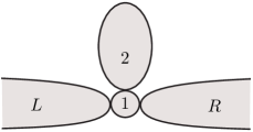
Figure 1: Device proposed in Ref. OGG, . Level spacing in the larger dot ($2$) must be negligibly small to allow for the NFL behavior of the device at low temperatures.

In principle, a setup having just one lead and two dots would allow one to study thermodynamic properties, such as magnetic susceptibility, in the 2CK regime. The existing technology kondo_exp , however, enables one to measure transport rather than thermodynamic properties. Therefore, two leads are needed to perform conductance measurements. In this paper, we assume that one of the electrodes is coupled weakly to the small dot and serves as a probe of the 2CK system formed by the two dots and the remaining electrode. We propose a detailed strategy for tuning the device to the NFL regime, and discuss various manifestations of NFL-related physics in the transport properties of the system.

II The Model

According to the discussion above, the device we consider consists of two quantum dots coupled to two conducting leads via single-mode junctions. The model Hamiltonian of such a device can be written as a sum of three parts,

$$H=H_{d}+H_{l}+H_{t}.$$ (1)

The first term here, $H_{d}$, describes an isolated system of two quantum dots, $1$ and $2$, connected via a single mode junction,

$$H_{d} = E_{1}\left(\sum_{s}d^{\dagger}_{s}d^{\phantom{\dagger}}_{s}-N\right)^{2}$$ (2)

$$+ \sum_{ks}\xi_{k}^{\phantom{\dagger}}\psi^{\dagger}_{2ks}\psi^{\phantom{\dagger}}_{2ks}+E_{2}\left(\sum_{ks}\psi^{\dagger}_{2ks}\psi^{\phantom{\dagger}}_{2ks}\right)^{2}$$

$$+ \sum_{ks}(t_{2}^{\phantom{\dagger}}\psi^{\dagger}_{2ks}d^{\phantom{\dagger}}_{s}+{\rm H.c.})$$

The last two terms in Eq. (1) represent the free electrons with spin $s=\pm 1$ in leads $R$ and $L$, and the tunneling between the leads and dot $1$, see Fig. 1,

$$H_{l} = \sum_{\alpha ks}\xi_{k}^{\phantom{\dagger}}c^{\dagger}_{\alpha ks}c^{\phantom{\dagger}}_{\alpha ks},\quad\alpha=R,L\,;$$ (3)

$$H_{t} = \sum_{\alpha ks}t_{\alpha}^{\phantom{\dagger}}c^{\dagger}_{\alpha ks}d^{\phantom{\dagger}}_{s}+{\rm H.c.}$$ (4)

In Eq. (2) the smaller dot (dot $1$) is described by a single-level system equivalent to the Anderson impurity model. The parameter $E_{1}$ represents charging energy, while the parameter $N$ is adjustable by tuning the potential on the capacitively coupled gate electrode. We neglect the finite level spacing $\delta E_{2}$ in the dot $2$, but account for its finite charging energy $E_{2}$ (we do not write explicitly the gate potential applied to the dot $2$, as it corresponds to a trivial shift of the chemical potential).

Since the relevant energies ($\omega\lesssim T_{K}$) for the Kondo effect are negligibly small compared to the Fermi energy, the electronic dispersion relation $\xi_{k}$ in Eqs. (2),(3) can be linearized: $\xi_{k}=v_{F}k$, where $k$ is measured from the Fermi momentum $k_{F}$. The linearization leads to an energy-independent density of states $\nu$, which will be assumed throughout this paper. Finally, we treat the tunneling amplitudes $t_{2},t_{R},t_{L}$ as real numbers and neglect their dependences on $k$. This is well justified for relevant values of $k$, $|k|\lesssim T/v_{F}$.

Instead of working with the operators $c_{R,L}$, it is convenient to introduce their linear combinations $\psi_{0,1}$,

$$\left(\begin{array}[]{c}\psi_{1ks}\\ \psi_{0ks}\end{array}\right)=\left(\begin{array}[]{cc}\cos\theta_{0}&\sin\theta_{0}\\ -\sin\theta_{0}&\cos\theta_{0}\end{array}\right)\left(\begin{array}[]{c}c_{Rks}\\ c_{Lks}\end{array}\right),$$ (5)

where the angle $\theta_{0}$ is determined by the equation

$$\tan\theta_{0}=t_{L}/t_{R}\;.$$ (6)

(So far there are no restrictions on the value of $t_{L}/t_{R}$.) The Hamiltonian (1)-(4) then assumes the “block-diagonal” form

$$H = H_{0}\{\psi_{0}\}+H_{1}\{\psi_{1},\psi_{2},d\},$$ (7)

$$H_{0} = \sum_{ks}\xi_{k}^{\phantom{\dagger}}\psi^{\dagger}_{0ks}\psi^{\phantom{\dagger}}_{0ks},$$ (8)

$$H_{1} = H_{d}\{\psi_{2},d\}+\sum_{ks}\xi_{k}^{\phantom{\dagger}}\psi^{\dagger}_{1ks}\psi^{\phantom{\dagger}}_{1ks}$$

$$~{}~{}~{}~{}~{}~{}~{}+\sum_{ks}(t_{1}^{\phantom{\dagger}}\psi^{\dagger}_{1ks}d^{\phantom{\dagger}}_{s}+{\rm H.c.}),$$

where $H_{d}\{\psi_{2},d\}$ is given by Eq. (2), and $t_{1}=\sqrt{t_{L}^{2}+t_{R}^{2}}$.

At low energies ($T\ll E_{1,2}$) the Hamiltonian $H_{1}$ involving the $\psi_{1}$ and $\psi_{2}$ operators, see Eq. (II), can be simplified further. Indeed, at $N\approx 1$ the small dot is occupied by a single electron, and, therefore, carries a spin $S=1/2$. The tunneling terms in Eqs. (2) and (II) mix the states with a single electron in in dot $1$ with states having $0$ or $2$ electrons in that dot. Because of the high energy cost ($\sim E_{1}$), these transitions are virtual, and, provided that the conductances of the corresponding junctions are small, can be taken into account perturbatively in the second order in tunneling amplitudes. A new OGG and important element here compared to the conventional treatment of the Anderson impurity model is that at $T\ll E_{2}$ only those excitations that conserve the number of electrons in dot $2$ are allowed. The resulting effective Hamiltonian which acts within the strip of energies $|\omega|\lesssim\min\{E_{1},E_{2}\}$, has the form of the 2CK model NB ; Bethe ; AJ ; Tsvelik ; AL ; CZ ,

$$H_{2CK}=\sum_{\gamma ks}\xi_{k}^{\phantom{\dagger}}\psi^{\dagger}_{\gamma ks}\psi^{\phantom{\dagger}}_{\gamma ks}+\sum_{\gamma}J_{\gamma}\left({\bf s}_{\gamma}\cdot{\bf S}\right)+BS^{z}.$$ (10)

Here the channel index $\gamma=1$ and $\gamma=2$ represents the leads and dot $2$, respectively, $\bf S$ is the spin-1/2-operator describing the doubly-degenerate ground state of dot $1$,

$${\bf s}_{\gamma}=\sum_{kk^{\prime}ss^{\prime}}\psi^{\dagger}_{\gamma ks}\frac{{\bm{\sigma}}_{ss^{\prime}}}{2}\psi^{\phantom{\dagger}}_{\gamma k^{\prime}s^{\prime}}$$

is the spin density in channel $\gamma$, and $\bm{\sigma}=(\sigma^{x},\sigma^{y},\sigma^{z})$ are the Pauli matrices. The exchange amplitudes $J_{\gamma}$ in Eq. (10) are estimated as

$$\nu J_{\gamma}=4\nu t_{\gamma}^{2}/E_{1}.$$ (11)

In derivation of Eq. (10), we assumed that the gate voltage is tuned precisely to $N=1$ (which corresponds to a particle-hole symmetric situation). As we discuss in Section V below, this assumption does not lead to qualitative changes in the results. We also included in the Hamiltonian the effect of an external magnetic field (hereinafter we omit the Bohr magneton $\mu_{B}$; the field $B$ is measured in the units of energy).

III Tunneling conductance

In order to study the out-of-equilibrium transport across the device we add to our Hamiltonian a term

$$H_{V}=\frac{eV}{2}\left(\hat{N}_{L}-\hat{N}_{R}\right),\quad\hat{N}_{\alpha}=\sum_{ks}c_{\alpha ks}^{\dagger}c_{\alpha ks}^{\phantom{\dagger}},$$ (12)

which describes a finite bias voltage $V$ applied between the left ($\alpha=L$) and right ($\alpha=R$) electrodes. The differential conductance $dI/dV$ can be evaluated in a closed form for arbitrary $V$ when one of the leads, say $L$, serves as a weakly coupled probe tutorial , i.e., $t_{L}\ll t_{R}$. Under this condition the angle $\theta_{0}$ in Eqs. (5) and (6) is small:

$$\theta_{0}\approx t_{L}/t_{R}\ll 1.$$ (13)

Application of the transformation Eq. (5) to Eq. (12), yields, to the linear order in $\theta_{0}$,

$$H_{V}=\frac{eV}{2}\left(\hat{N}_{0}-\hat{N}_{1}\right)+eV\theta_{0}\sum_{ks}(\psi^{\dagger}_{0ks}\psi^{\phantom{\dagger}}_{1ks}+{\rm H.c.}),$$ (14)

where

$$\hat{N}_{0}=\sum_{ks}\psi^{\dagger}_{0ks}\psi^{\phantom{\dagger}}_{0ks},\quad\hat{N}_{1}=\sum_{ks}\psi^{\dagger}_{1ks}\psi^{\phantom{\dagger}}_{1ks}.$$

The first term on the right-hand side of Eq. (14) can be interpreted as a voltage bias between the reservoirs of $0$- and $1$-particles, cf. Eq. (12), while the second term has an appearance of the $k$-conserving tunneling. Since the tunneling amplitude is proportional to the small parameter $\theta_{0}\ll 1$, see Eq. (13), one can use perturbation theory to calculate the current across the device tutorial .

Similar to the representation of $H_{V}$ in the form of Eq. (14), the current operator

$$\hat{I}=\frac{d}{dt}\frac{e}{2}\left(\hat{N}_{R}-\hat{N}_{L}\right)$$

also splits naturally into two contributions,

$$\hat{I}=\hat{I}_{0}+\delta\hat{I}.$$ (15)

Here

$$\hat{I}_{0} = \frac{d}{dt}\frac{e}{2}\left(\hat{N}_{1}-\hat{N}_{0}\right)$$

$$= ie^{2}V\theta_{0}\sum_{ks}\psi_{0ks}^{\dagger}\psi_{1ks}^{\phantom{\dagger}}+{\rm H.c.},$$

is a current between the reservoirs of $0$- and $1$-particles, and

$$\delta\hat{I}=-e\theta_{0}\frac{d}{dt}\sum_{ks}\psi^{\dagger}_{0ks}\psi^{\phantom{\dagger}}_{1ks}+{\rm H.c.}$$ (17)

It is easy to show tutorial that in the leading (second) order in $\theta_{0}$ the operator $\delta\hat{I}$ does not contribute to the average current across the device. The remaining contribution $\langle\hat{I}_{0}\rangle$ corresponds to the $k$-conserving tunneling between two bulk reservoirs containing $0$- and $1$-particles, see Eqs. (14) and (III). Its evaluation yields tutorial

$$\frac{dI}{dV}=G_{0}\sum_{s}\frac{1}{2}\int d\omega(-df/d\omega)\left[-\pi\nu{\rm Im}T_{1s}(\omega+eV)\right]$$ (18)

for the differential conductance. Here $f(\omega)$ is the Fermi function ($\omega$ is the energy measured from the Fermi level),

$$G_{0}=\frac{2e^{2}}{h}(2\theta_{0})^{2}\approx\frac{8e^{2}}{h}\frac{t_{L}^{2}}{t_{R}^{2}},$$ (19)

and $T_{1s}$ is the t-matrix for the particles of channel $\gamma=1$ [evaluated with the equilibrium Hamiltonians Eq. (II) or Eq. (10)]. The t-matrix is related to the exact retarded Green function $G_{ks,k^{\prime}s^{\prime}}=\delta_{ss^{\prime}}G_{ks,k^{\prime}s}$ of these particles according to

$$G_{ks,k^{\prime}s}=G^{0}_{k}+G^{0}_{k}T_{1s}^{\phantom{0}}G^{0}_{k^{\prime}},\quad G^{0}_{k}=(\omega-\xi_{k}+i0)^{-1}.$$

Here we took into account the conservation of the total spin, which implies that $G_{ks,k^{\prime}s^{\prime}}$ is diagonal in $s,s^{\prime}$. In our model with $t_{1}$ independent of $k$ (and, consequently, $J_{1}$ independent of $k$ and $k^{\prime}$), the t-matrix is also independent of $k,k^{\prime}$. Note that the linear response ($V\to 0$) counterpart of Eq. (18), the linear conductance

$$G=G_{0}\sum_{s}\frac{1}{2}\int d\omega(-df/d\omega)\left[-\pi\nu{\rm Im}T_{1s}(\omega)\right],$$ (20)

remains valid tutorial for an arbitrary relation between $t_{L}$ and $t_{R}$, in which case $G_{0}=(2e^{2}/h)\sin^{2}(2\theta_{0})$.

IV Transport at finite temperature and bias

Equation (18) provides a direct link between the measurable quantity, the differential conductance $dI/dV$, and the properties of the 2CK model, Eq. (10). In the channel-symmetric case $J_{1}=J_{2}=J$ the NFL behavior manifests itself in a nonanalytic dependence of the t-matrix on energy and temperature AL , which leads to a rather unusual scaling of the differential conductance at low bias and temperature ($|eV|,T\ll T_{K}$):

$$\frac{1}{G_{0}}\frac{dI}{dV}=\frac{1}{2}\left[1-\sqrt{\frac{\pi T}{T_{K}}}F_{\rm 2CK}\left(\frac{|eV|}{\pi T}\right)\right].$$ (21)

The function $F_{\rm 2CK}(x)$ here is a universal (parameter-free) scaling function AL with the asymptotes

$$F_{\rm 2CK}(x)=\left\{\begin{array}[]{lr}1+cx^{2},&x\ll 1\\ \displaystyle\frac{3}{\sqrt{\pi}}\sqrt{x},&x\gg 1\end{array}\right.,$$ (22)

where $c$ is a numerical coefficient of the order of $1$. The limit $eV/T\to 0$ of Eq. (21) yields

$$G=G_{0}\frac{1}{2}\left(1-\sqrt{\pi T/T_{K}}\right)$$ (23)

for the linear conductance (this result is valid for arbitrary value of $t_{L}/t_{R}$). The estimate scales of the Kondo temperature $T_{K}$ introduced in Eqs. (21) and (23) reads CZ

$$T_{K}\sim E_{0}(\nu J)e^{-1/J\nu},\qquad E_{0}=\min\{E_{1},E_{2}\}.$$ (24)

The validity of Eqs. (21) and (23) is limited by the requirements that both the Zeeman energy $B$ and the level spacing $\delta E_{2}$ are small compared to $T$, and that the exchange constants in Eq. (10) are equal to each other: $J_{1}=J_{2}$. When the system is tuned away from this special point, at a finite

$$\Delta=\nu J_{1}-\nu J_{2},$$ (25)

the conductance changes drastically. In the ideal case of $T=0$ and $\delta E_{2}=0$, the conductance has a step-like dependence on $\Delta$,

$$G(\Delta)=G_{0}\theta(\Delta).$$ (26)

The discontinuity in Eq. (26) reflects a quantum phase transition between two different Fermi liquid (FL) states, in which the spin of the dot $1$ forms a singlet with either the collective spin of the electrons in the leads (FL1, $\Delta>0$) or with that of the dot $2$ (FL2, $\Delta<0$). At the critical point $\Delta=0$, the system exhibits NFL behavior down to $T=0$. In agreement with the general theory of quantum phase transitions Sachdev , the $T\to 0$ asymptotics at $|\Delta|\neq 0$ corresponds to the FL, whereas the NFL behavior Eq. (23) is preserved at temperatures well above certain $\Delta$-dependent crossover scale $T_{\Delta}$, see Fig. 2. By the same token, the step in the $\Delta$-dependence of $G(\Delta)$, Eq. (26), is smeared at finite temperatures.

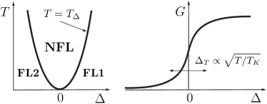
Figure 2: Quantum phase transition between two FL states. The NFL behavior is preserved at $|\Delta|\neq 0$, provided the temperature exceeds the crossover scale $T_{\Delta}$, see Eq. (31). The width $\Delta_{T}$ of step in the conductance $G(\Delta)$ scales with temperature as $\sqrt{T}$, see Eq. (34).

In order to estimate scales the energy scale $T_{\Delta}$ we consider the renormalization group (RG) flow of the effective exchange constants as the high-energy cutoff $D$ is reduced from its initial value $D_{0}\sim E_{0}$. We are interested in the case when the bare value of $\Delta$ is small,

$$|\Delta|\ll{\cal J},$$

where

$${\cal J}=\nu(J_{1}+J_{2})/2\,.$$ (27)

The evolution of the effective coupling constants ${\cal J}^{*},\Delta^{*}$ with the decrease of $D$ is then described by the Poor Man’s scaling equations PWA_book

$$\frac{d{\cal J}^{*}}{d\zeta}=({\cal J}^{*})^{2},\quad\frac{d\Delta^{*}}{d\zeta}=2{\cal J}^{*}\Delta^{*},\quad\zeta=\ln\frac{D_{0}}{D}$$ (28)

with the initial conditions

$${\cal J}^{*}(D_{0})={\cal J},\quad\Delta^{*}(D_{0})=\Delta.$$

Equations (28) are valid as long as $\Delta^{*}\ll{\cal J}^{*}\ll 1$ and yield the relation $\Delta^{*}/\Delta=({\cal J}^{*}/{\cal J})^{2}$. By the time ${\cal J}^{*}$ has grown to be of the order of $1$ at $D\sim T_{K}$, the value of $\Delta^{*}$ characterizing the channel asymmetry reaches

$$\Delta^{*}(T_{K})\sim\Delta/{\cal J}^{2}.$$ (29)

This can be viewed as the initial (at $D\sim T_{K}$) value of the coupling constant of the relevant NB ; ALPC channel-symmetry-breaking perturbation. The perturbation will eventually drive the system away from the 2CK fixed point at $D\to 0$. However, if $\Delta^{*}(T_{K})\ll 1$, then one expects the behavior of the system in a broad range of energies to be still governed by the vicinity of the 2CK fixed point. The channel anisotropy is a relevant operator with scaling dimension $1/2$, see Ref. ALPC, . Hence, the dependence of the corresponding coupling constant $\Delta^{*}$ on $D$ is described by

$${\Delta^{*}(D)\over\Delta^{*}(T_{K})}\propto\left({T_{K}\over D}\right)^{1/2}.$$ (30)

The condition $\Delta^{*}(T_{\Delta})\sim 1$, together with Eq. (29), then gives the estimate

$$T_{\Delta}\sim[\Delta^{*}(T_{K})]^{2}T_{K}\sim\left({\Delta^{2}}/{{\cal J}^{4}}\right)T_{K}.$$ (31)

The RG flow stops at $D\sim\max\{T,|eV|\}$. Consequently, at $\max\{T_{\Delta},|eV|\}\ll T\ll T_{K}$, the channel asymmetry yields a small correction to the conductance Eq. (23). The correction is first order in the corresponding perturbation, hence proportional to $\Delta^{*}(T)\sim(T_{\Delta}/T)^{1/2}$, and its sign is determined by the sign of $\Delta$:

$$\delta G/G_{0}\propto{\rm sgn}(\Delta)\left(\frac{T_{\Delta}}{T}\right)^{1/2}.$$ (32)

On the other hand, for $T,|eV|\ll T_{\Delta}$ the system is a Fermi liquid, see Fig. 2. Substitution of the t-matrix in the form

$$-\pi\nu{\rm Im}~{}T_{1s}=\theta(\Delta)-{\rm sgn}(\Delta)\frac{3\omega^{2}+\pi^{2}T^{2}}{2T_{\Delta}^{2}}$$

[cf. Ref. AL, ] into Eq. (18) then yields

$$\frac{1}{G_{0}}\frac{dI}{dV}=\theta(\Delta)-{\rm sgn}(\Delta)\left(\frac{\pi T}{T_{\Delta}}\right)^{2}\left[1+\frac{3}{2}\left(\frac{eV}{\pi T}\right)^{2}\right].$$ (33)

Again, the linear response ($V\to 0$) counterpart of Eq. (33) is valid at any ratio $t_{L}/t_{R}$. The temperature dependence of the linear conductance at fixed small values of $\Delta$ is sketched in Fig. 3.

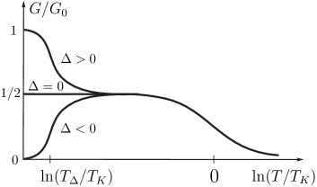
Figure 3: Sketch of the temperature dependence of the linear conductance at fixed values of $\Delta$ and $T_{K}$. For $\Delta<0$ the dependence is nonmonotonic, with a maximum at $T\sim\sqrt{T_{\Delta}T_{K}}$. At $T\gg T_{K}$ the conductance scales as $G/G_{0}\propto[\ln(T/T_{K})]^{-2}$, see, e.g., Ref. tutorial, .

According to Eq. (33), corrections to the zero-temperature limit of the linear conductance, the step-function Eq. (26), are quadratic in temperature – a typical Fermi-liquid result Nozieres . At a finite temperature, the step-function is smeared, see Fig. 2. The characteristic width $\Delta_{T}$ of the smeared step at temperature $T$ is estimated by solving the equation $T_{\Delta}\sim T$ for $\Delta$, which results in

$$\Delta_{T}\sim{\cal J}^{2}\sqrt{T/T_{K}}.$$ (34)

This “sharpening” of the $\Delta$-dependence of the linear conductance with decreasing temperatures (see Fig. 2) can be regarded as a “smoking gun” for non-Fermi-liquid behavior. In fact, it might be easiest to first identify unambiguously the step-like dependence of the conductance on $\Delta$ and then use it to tune the device precisely to the symmetry point in order to observe the distinctive scaling of the differential conductance Eq. (21). Experimentally, the value of $\Delta$ is controlled OGG by the asymmetry of the conductances of the corresponding tunneling junctions, which in turn are controlled by the potentials $V_{g}$ on the gates forming the junctions. In the vicinity of the symmetry point, the dependence of $G$ on $V_{g}$ should have the form of a smeared step-function, whose width $\delta V_{g}$ should scale with temperature as $\sqrt{T}$, see Fig. 2.

V Linear conductance at a finite magnetic field

The magnetic field dependence of the linear conductance across the device also reveals the critical behavior. In this Section we study the dependence $G(B)$ at $T=0$ in the vicinity of the quantum critical point $\Delta=0$. We consider only the Zeeman effect of the magnetic field, and dispense with its orbital effect (this is an adequate approximation for a field applied in the plane of a lateral quantum dot device).

Similar to the effect of a finite temperature, see Fig. 2, the application of a magnetic field at small $\Delta$ results in a crossover from the limiting FL behavior at $B\to 0$ to NFL intermediate regime at higher fields $B\gtrsim B_{\Delta}$. As before, the crossover scale $B_{\Delta}$ can be estimated scales from RG arguments. The scaling dimension ALPC of the operator $S^{z}$ in Eq. (10) at the 2CK fixed point is $1/2$. Accordingly, when the high energy cutoff $D$ is lowered, the effective splitting of the impurity levels $B^{*}$ evolves according to

$${B^{*}(D)/D\over B^{*}(T_{K})/T_{K}}\propto\left(\frac{T_{K}}{D}\right)^{1/2}$$ (35)

with the initial condition $B^{*}(T_{K})\sim B$. The RG flow Eq. (35) terminates once $B^{*}$ has grown to become of the order of $D$, or when $D$ reaches the value $T_{\Delta}$, whichever occurs at a higher value of $D$. The first of the two conditions corresponds to the limitation on the NFL behavior set by the Zeeman splitting, while the second one is due to the channel anisotropy. Therefore, the crossover scale $B_{\Delta}$ can be estimated as that field $B\sim B^{*}(T_{K})$ in Eq. (35), at which $B^{*}(D)\sim D$ and $D\sim T_{\Delta}$ simultaneously. Using Eqs. (35) and (31), we find the relation between the crossover field AJ , the crossover temperature $T_{\Delta}$, and the channel anisotropy parameter $\Delta$

$$B_{\Delta}\sim\sqrt{T_{\Delta}T_{K}}\sim\left({|\Delta|}/{\cal J}^{2}\right)T_{K}.$$ (36)

Note the difference between the $\Delta$–dependence of the crossover temperature $T_{\Delta}$ [Eq. (31)] and the crossover field $B_{\Delta}$.

Having found the crossover scale $B_{\Delta}$, next we investigate the dependence of the conductance $G$ on the field $B$. First of all, we note that at $\Delta\neq 0$ the low-energy properties of the Hamiltonian Eq. (10) are those of a Fermi liquid.NB The effect of any local perturbation, such as the exchange interaction with the spin of the dot $1$ in Eq. (10), on the ground state of the Fermi liquid is completely characterized by the scattering phase shifts $\delta_{\gamma s}$ at the Fermi level. (Recall that $s=\pm 1$ for spin-up/down and $\gamma=1,2$ labels the two channels.) The t-matrix that enters Eq. (20) is then given by the standard scattering theory expression

$$-\pi\nu T_{\gamma s}(0)=\frac{1}{2i}\left(e^{2i\delta_{\gamma s}}-1\right).$$ (37)

Obviously, the phase shifts are defined only mod $\pi$ (that is, $\delta_{\gamma s}$ is equivalent to $\delta_{\gamma s}+\pi$ ). The ambiguity is removed by setting the values of the phase shifts corresponding to $J_{\gamma}=0$ in Eq. (10) to zero. With this convention, the invariance of the Hamiltonian (10) with respect to the particle-hole transformation $\psi_{\gamma ks}\to\psi^{\dagger}_{\gamma,-k,-s}$ translates into the relation

$$\delta_{\gamma s}+\delta_{\gamma,-s}=0$$ (38)

for the phase shifts, which suggests a representation

$$\delta_{\gamma s}=s\delta_{\gamma}.$$ (39)

Substitution of Eqs. (37) and (39) into Eq. (20) yields

$$G/G_{0}=\frac{1}{2}\sum_{s}\sin^{2}\delta_{1s}=\sin^{2}\delta_{1}$$ (40)

for the linear conductance at $T=0$. In the limit $B/T_{K}\to+0$ and at $\Delta\neq 0$, the ground state of the Hamiltonian (10) is a singlet. Therefore, the total spin in a very large but finite region of space surrounding the dot $1$ is zero. By the Friedel sum rule, this implies relation $\sum_{\gamma s}s\delta_{\gamma s}=\pi$. Taking, in addition, Eq. (39) into account, one obtains relation

$$\delta_{1}+\delta_{2}=\pi/2,$$ (41)

valid at any value of $B/B_{\Delta}$, as long as $B\ll T_{K}$.

Below the crossover, $B\ll B_{\Delta}$, the values of the phase shifts are determined by the vicinity of the stable Fermi-liquid fixed points NB , $\delta_{1}=\pi/2$, $\delta_{2}=0$ at $\Delta>0$ and $\delta_{1}=0$, $\delta_{2}=\pi/2$ at $\Delta<0$. Substitution of these values into Eq. (40) then yields Eq. (26) for the conductance. The corrections to the fixed point values of the phase shifts are linear in $B/B_{\Delta}$,

$$\delta_{1}=\pi/2-\delta_{2}=(\pi/2)\theta(\Delta)-{\rm sgn}(\Delta)(B/B_{\Delta}),$$ (42)

yielding

$$G/G_{0}=\theta(\Delta)-{\rm sgn}(\Delta)(B/B_{\Delta})^{2},\quad B\ll B_{\Delta}$$ (43)

[cf. Eq. (33)].

Above the crossover, i.e., for $B_{\Delta}\ll B\ll T_{K}$, the departure of the phase shifts from the 2CK fixed point values $\delta_{1,2}=\pi/4$ is controlled by the properties of the fixed point. To account for a finite value of $B/T_{K}$, we generalize Eq. (41):

$$\delta_{1}+\delta_{2}=\pi\left[1/2+M(B)\right].$$

The zero-temperature magnetization $M(B)$ here is known exactly from the Bethe-ansatz solution Bethe ; AJ ; SS . Using the asymptote SS $M(B)\propto(B/T_{K})\ln(T_{K}/B)$, we find

$$\delta_{1}={\pi\over 4}+\,a\,{\rm sgn}(\Delta){B_{\Delta}\over B}-b{B\over T_{K}}\ln{T_{K}\over B}.$$ (44)

Here $a$ and $b$ are positive numerical coefficients of the order of $1$. The second term on the right-hand side of Eq. (42) is the first-order correction in the channel-symmetry-breaking perturbation. This correction is similar to Eq. (32) with temperature $T$ replaced by the energy scale $D^{*}(B)\sim B^{2}/T_{K}$ at which the RG flow defined by Eq. (35) terminates. Equations (44) and (40) yield the asymptote of the conductance at $B_{\Delta}\ll B\ll T_{K}$,

$$\frac{G}{G_{0}}=\frac{1}{2}+\,a\,{\rm sgn}(\Delta)\frac{B_{\Delta}}{B}-b\frac{B}{T_{K}}\ln\frac{T_{K}}{B}.$$ (45)

The shape of $G(B)$ is qualitatively similar to that of $G(T)$, see Eqs. (23),(32), and (33), although the precise functional form is rather different.

Interestingly, in the case of small channel anisotropy, $T_{\Delta}\ll T_{K}$, there is an approximate symmetry with respect to the change of sign of $\Delta$:

$$G(B,\Delta)+G(B,-\Delta)=2G(B,\Delta\to 0).$$ (46)

Note that this relation is valid at any $B/T_{K}$, provided that $T_{\Delta}/T_{K}\ll 1$.

Strictly speaking, the consideration of this Section is applicable only at zero temperature. However, the results Eqs. (43) and (45) remain valid CZ as long as

$$T\ll B^{2}/T_{K}$$ (47)

At higher temperatures the conductance is described by the corresponding expressions of Section IV. As follows from Eqs. (23) and (45), the limiting value of the linear conductance at the 2CK fixed point, $G=G_{0}/2$, is independent of the order in which the limits $B\to 0$, $T\to 0$ are taken nCK . Hence, the crossover between the field-dominated regime, see Eqs. (43) and (45), and the temperature-dominated one, see Eqs. (23), (32) and (33), is expected to be smooth and featureless.

For arbitrary values of $T_{\Delta}/T_{K}$, the detailed magnetic field dependence of the phase shifts at the Fermi level can be studied using the numerical renormalization group (NRG) Wilson . In this approach one defines a sequence of discretized Hamiltonians and diagonalizes them iteratively to obtain the finite-size spectrum of the model. In the Fermi liquid case ($\Delta\neq 0$) knowledge of the finite-size spectrum is sufficient to identify unambiguously the phase shifts ALPC .

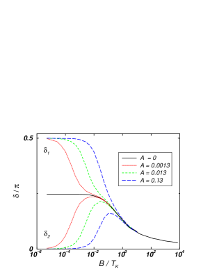
Figure 4: The phase shifts for the 2CK model at different values of the channel asymmetry parameter $A=\Delta/{\cal J}^{2}$. The upper (lower) curves represent $\delta_{1}(\delta_{2})$.

In Fig. 4, we plotted the phase shifts $\delta_{1,2}$ as a function of $B$ for different values of the parameter $A=\Delta/{\cal J}^{2}>0$ that characterizes the asymmetry between the channels. We estimate the crossover scales scales $T_{K}$ and $B_{\Delta}$ as the two values of $B$ in Fig. 4 at which the phase shift $\delta_{2}$ equals $\pi/8$. In order to verify the relation $B_{\Delta}/T_{K}\sim A$, see Eq. (36), we plotted $B_{\Delta}$ vs $A$ on the left panel in Fig. 5. The NRG data also allow us to estimate the scale $T_{\Delta}$, see Eq. (31), as the energy scale at which the first excited state of the NRG spectrum has reached the halfway mark of its crossover evolution between the corresponding two fixed point values, see Fig. 5, right panel. The NRG data are very well described by $B_{\Delta}/T_{K}\approx 0.5A$, $T_{\Delta}/T_{K}\approx 4A^{2}$, in agreement with Eqs. (36) and (31) above.

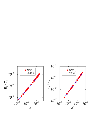
Figure 5: Dependences of the crossover scales $B_{\Delta}$ and $T_{\Delta}$ on the asymmetry parameter $A=\Delta/{\cal J}^{2}$.

Having extracted the phase shifts, we are able to calculate the linear conductance from Eqs. (40) and (46), see Fig. 6. As expected, the conductance develops a signature of a plateau at intermediate values of the field $B_{\Delta}<B<T_{K}$. At very high fields, $B\gg T_{K}$, the conductance scales with $B$ as $1/\ln^{2}(B/T_{K})$.

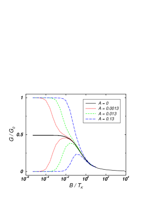
Figure 6: Field dependence of the conductance at different values of the asymmetry parameter $A=\Delta/{\cal J}^{2}$. The upper (lower) curves correspond to $A>0$ ($A<0$).

As usual in NRG calculations, we measured all energies in units of the bandwith $D$. In order to avoid the disturbing finite bandwidth effects, we used two different coupling constants for the high- and low-field regimes: one set of data, that includes the $B\gg B_{\Delta}$ regime, was obtained using ${\cal J}=0.075$, while another set of data, which includes the $B\ll T_{K}$ regime, was obtained using ${\cal J}=0.15$. The two sets were combined by rescaling the magnetic field in units of the Kondo temperature, resulting in a set of continuous curves, as shown in the figures. The overlap of the two sets of data at intermediate fields confirms that in this regime the accuracy of our numerics is remarkably good. Based on the dependence on the finite system size, we estimate the relative error of the calculated phase shifts to be of the order of $2\%$. (The worst case is the low field part of the $A=0$ curve, because of the extremely fragile nature of the intermediate NFL fixed point.)

VI Effect of Potential Scattering

So far we concentrated on the particle-hole symmetric model. In general, however, such symmetry is absent. It is violated by the presence of higher energy levels in dot $1$, and also by deviations of the dimensionless gate voltage $N$ from an integer value. In the absence of particle-hole symmetry, the effective Hamiltonian (10) acquires additional terms leading to potential scattering. Taking into account that the interchannel scattering is blocked at energies well below $E_{1,2}$, we can write this additional perturbation as

$$H_{p}=\sum_{\gamma=1,2}V_{\gamma}\sum_{kk^{\prime}s}\psi^{\dagger}_{\gamma ks}\psi^{\phantom{\dagger}}_{\gamma k^{\prime}s}.$$ (48)

Including $H_{p}$ into our considerations leads to a modification of the limiting values of the conductance in the Fermi-liquid and 2CK fixed points. The dependences of $dI/dV$ on $\Delta,V,T$ and $B$, however, remain the same apart from acquiring a constant background contribution $G_{el}$ due to elastic cotunneling. Here we illustrate this for a specific example of the zero-temperature magnetoconductance.

The potential scattering yields finite spin-independent phase shifts $\delta_{\gamma}^{0}=-\arctan(\pi\nu V_{\gamma})$ even if $J_{\gamma}$ in Eq. (10) are set to $0$. This can be accounted for by a proper modification N of Eq. (39),

$$\delta_{\gamma s}=\delta_{\gamma}^{0}+s\delta_{\gamma},$$ (49)

where the dependence of $\delta_{\gamma}$ on $B$ and $\Delta$ is described by the ”particle-hole symmetric” expressions (42) and (44). Substitution of the phase shifts in the form of Eq. (49) into Eq. (40) results in real

$$G(B,\Delta)=G_{el}+{\widetilde{G}}_{0}F[B/B_{\Delta},B/T_{K},{\rm sgn}(\Delta)],$$ (50)

where $G_{el}=G_{0}\sin^{2}\delta^{0}_{1}$, the function $F$ is a universal function with asymptotes given in Eqs. (43) and (45), and ${\widetilde{G}}_{0}=G_{0}-2G_{el}$. Note that the limiting value of the conductance at the 2CK fixed point, $G_{el}+{\widetilde{G}}_{0}/2$, lies precisely half-way between the two Fermi-liquid limits, $G_{el}$ and $G_{el}+{\widetilde{G}}_{0}$, and that Eq. (46) remains valid even in the presence of the potential scattering Eq. (48).

VII Discussion

The low-temperature properties of a quantum dot device normally are well described by Fermi liquid theory. The special two-dot structure proposed in Ref. OGG, allows, however, for NFL behavior at a special point in the space of parameters of the device. In the context of the physics of quantum phase transitions, this point can be viewed as a critical point separating two Fermi liquid states. In this paper, we developed a detailed theory of the transport properties near such a quantum critical point. Our theory offers a strategy for tuning the device parameters to the critical point characterized by the two-channel Kondo effect physics, by monitoring the temperature dependence of the linear conductance, see Sec. IV. Further confirmation of the 2CK behavior may come from the measurements of the differential conductance, which must display universal behavior, see Sec. IV. We also investigated the effect of magnetic field and of potential scattering on the conductance in the vicinity of the quantum critical point, see Secs. V and VI. The Zeeman splitting allows one to investigate the finite-field crossover between the Fermi liquid and NFL behavior of the conductance. In the vicinity of the NFL point, the linear conductance of the device depends on the magnetic field and temperature only via two dimensionless parameters, $T/T_{\Delta}$ and $B/B_{\Delta}$; the dependence of $T_{\Delta}$ and $B_{\Delta}$ on the channel asymmetry $\Delta$ is given in Eqs. (31) and (36). Note also that potential scattering does not destroy the 2CK behavior, but merely renormalizes the magnitude of the Kondo contribution to the conductance. A finite level spacing in the larger dot $\delta E_{2}$, however, is a hazard. At temperatures below $\delta E_{2}$ the two-dot device inevitably enters into the conventional Fermi-liquid regime.

- (1) Y. Oreg and D. Goldhaber-Gordon, Phys. Rev. Lett. 90, 136602 (2003).
- (2) P.W. Anderson, Basic Notions of Condensed Matter Physics (Addison-Wesley, Reading, 1997).
- (3) P. Nozières, J. Low Temp. Phys. 17, 31 (1974).
- (4) A.I. Larkin and V.I. Melnikov, Zh. Eksp. Teor. Fiz. 61, 1231 (1971) [Sov. Phys. JETP 34, 656 (1972)].
- (5) P. Nozières and A. Blandin, J. Physique 41, 193 (1980).
- (6) P. B. Wiegmann and A. M. Tsvelick, Pis’ma Zh. Eksp. Teor. Fiz. 38, 489 (1983) [JETP Lett. 38, 591 (1983)]; A.M. Tsvelick and P.B. Wiegmann, J. Phys. C 17, 2321 (1983); A.M. Tsvelick, J. Phys. C 18, 159 (1985); N. Andrei and C. Destri, Phys. Rev. Lett. 52, 364 (1984);
- (7) N. Andrei and A. Jerez, Phys. Rev. Lett. 74, 4507 (1995).
- (8) A.M. Tsvelick, J. Phys.: Condens. Matter 2, 2833 (1990).
- (9) I. Affleck and A.W.W. Ludwig, Phys. Rev. B 48, 7297 (1993).
- (10) D.L. Cox and A. Zawadowski, Adv. Phys. 47, 599 (1998).
- (11) I.L. Aleiner, B.L. Altshuler, Y.M. Galperin, and T.A. Shutenko, Phys. Rev. Lett. 86, 2629 (2001).
- (12) K.A. Matveev, Phys. Rev. B 51, 1743 (1995); K.A. Matveev, Zh. Eksp. Teor. Fiz. 99, 1598 (1991) [Sov. Phys. JETP 72, 892 (1991)].
- (13) L.I. Glazman, F.W.J. Hekking, and A.I. Larkin, Phys. Rev. Lett. 83, 1830 (1999).
- (14) A. Furusaki and K.A. Matveev, Phys. Rev. B 52, 16676 (1995).
- (15) D. Goldhaber-Gordon, H. Shtrikman, D. Mahalu, D. Abusch-Magder, U. Meirav, and M.A. Kastner, Nature (London) 391, 156 (1998); S.M. Cronenwett, T.H. Oosterkamp, and L.P. Kouwenhoven, Science 281, 540 (1998); J. Schmid, J. Weis, K. Eberl, and K. von Klitzing, Physica (Amsterdam) 256B-258B, 182 (1998); W.G. van der Wiel, S. De Franceschi, T. Fujisawa, J.M. Elzerman, S. Tarucha, and L.P. Kouwenhoven, Science 289, 2105 (2000).
- (16) M. Pustilnik and L.I. Glazman, Phys. Rev. Lett. 87, 216601 (2001).
- (17) L.I. Glazman and M. Pustilnik, in New Directions in Mesoscopic Physics (Towards Nanoscience), edited by R. Fazio, V.F. Gantmakher, and Y. Imry (Kluwer, Dordrecht, 2003), pp. 93-115 (preprint cond-mat/0302159).
- (18) The definitions of the crossover scales , and adopted in this paper are based on the asymptotic behavior of the linear conductance at low and , see Eqs. (23), (33) and (43), correspondingly.
- (19) S. Sachdev, Quantum Phase Transitions (Cambridge University Press, 1999).
- (20) I. Affleck, A.W.W. Ludwig, H.-B. Pang, and D.L. Cox, Phys. Rev. B 45, 7918 (1992).
- (21) P.D. Sacramento and P. Schlottmann, Phys. Rev. B 43, 13294 (1991)
- (22) Note that if the number of channels is larger than , the value of the conductance at and depends on the order in which the limits are taken. This property is easy to understand in the limit of very large number of channels when the NFL fixed point lies within the reach of perturbation theory NB ; AL ; FR .
- (23) S. Florens and A. Rosch, cond-mat/0311219.
- (24) K.G. Wilson, Rev. Mod. Phys. 47, 773 (1975).
- (25) P. Nozières, J. Physique 39, 1117 (1978).