Dissipation in Josephson qubits

Abstract

Josephson-junction systems have been studied as potential realizations of quantum bits. For their operation as qubits it is crucial to maintain quantum phase coherence for long times. Frequently relaxation and dephasing effects are described in the frame of the Bloch equations. Recent experiments demonstrate the importance of $1/f$ noise, or operate at points where the linear coupling to noise sources is suppressed. This requires generalizations and extensions of known methods and results. In this tutorial we present the Hamiltonian for Josephson qubits in a dissipative environment and review the derivation of the Bloch equations as well as systematic generalizations. We discuss $1/f$ noise, nonlinear coupling to the noise source, and effects of strong pulses on the dissipative dynamics. The examples illustrate the renormalization of qubit parameters by the high-frequency noise spectrum as well as non-exponential decay governed by low-frequency modes.

1 Introduction

Quantum-state engineering requires coherent manipulations of suitable quantum systems. The needed quantum manipulations can be performed if we have sufficient control over the fields which couple to the quantum degrees of freedom, as well as the interactions. The effects of external noise sources have to be minimized in order to achieve long phase coherence times. In this tutorial we review the requirements for suitable physical realizations of qubits – with emphasis on Josephson circuits – and discuss ways to analyze the dissipative effects.

As has been stressed by DVD-Curacao any physical system, considered as a candidate for quantum computation, should satisfy the following five criteria: (i) One needs well-defined two-state quantum systems (qubits). (ii) One should be able to prepare the initial state of the qubits with sufficient accuracy. (iii) A long phase coherence time is needed, sufficient to allow for a large number (depending on details, say, $\geq 10^{4}$) of coherent manipulations. (iv) Control over the qubits’ Hamiltonian is required to perform the necessary unitary transformations. (v) Finally, a quantum measurement is needed to read out the quantum information.

The listed requirements may be satisfied by a system of spins – or quantum degrees of freedom which under certain conditions effectively reduce to two-state quantum systems – which are governed by a Hamiltonian of the form

$$H=H_{\rm ctrl}(t)+H_{\rm meas}(t)+H_{\rm res}\ .$$ (1)

The first term, $H_{\rm ctrl}(t)$, describes the control fields and interactions,

$$H_{\rm ctrl}(t)=-\frac{1}{2}\sum\limits_{i,a}B^{i}_{a}(t)\sigma^{i}_{a}+\sum\limits_{i\neq j;a,b}J^{ij}_{ab}(t)\sigma_{a}^{i}\sigma_{b}^{j}\;.$$ (2)

Here $\sigma_{a}$ (with $a,b=x,y,z$) are Pauli matrices in the basis of states $\left|\uparrow\right\rangle=\left(1\atop 0\right)$ and $\left|\downarrow\right\rangle=\left(0\atop 1\right)$. Full control of the unitary quantum dynamics of individual spins is achieved if the effective ‘magnetic field’ $\vec{B}^{i}(t)$ can be switched arbitrarily at each site $i$. For most purposes control over two of the field components is sufficient, e.g., $H_{\rm ctrl}(t)=-\frac{1}{2}\sum\limits_{i}\left[B^{i}_{z}(t)\sigma^{i}_{z}+B^{i}_{x}(t)\sigma^{i}_{x}\right]$. In order to perform logic operations, e.g. for quantum computing, one also needs two-qubit operations. They can be controlled if the coupling, $J^{ij}_{ab}(t)$, between the qubits can be switched. Examples for a suitable coupling are an Ising $zz$-coupling or a spin-flip $xy$-coupling (see below).

The measurement device and the residual interactions with the environment are accounted for by extra terms $H_{\rm meas}(t)$ and $H_{\rm res}$, respectively. Ideally the measurement device should be switchable as well and be kept in the off-state during manipulations. The residual interaction $H_{\rm res}$ leads to dephasing and relaxation processes. It has to be weak in order to allow for a series of coherent manipulations.

A typical experiment involves preparation of an initial quantum state, switching the fields $\vec{B}^{i}(t)$ and coupling energies $J^{ij}_{ab}(t)$ to effect a specified unitary evolution of the wave function, and the measurement of the final state.

The initial state can be prepared by keeping the system at low temperatures in strong enough fields, $B^{i}_{z}\gg k_{\rm B}T$, for sufficient time such that the residual interaction, $H_{\rm res}$, relaxes each qubit to its ground state, $\left|\uparrow\right\rangle$.

A single-bit operation on a selected qubit $i$ can be performed, e.g., by turning on the field $B^{i}_{x}(t)$ for a time span $\tau$. As a result the spin state evolves according to the unitary transformation

$$U^{i}_{x}\left(\alpha\right)=\exp\left(\frac{iB^{i}_{x}\tau\sigma^{i}_{x}}{2\hbar}\right)=\left(\begin{array}[]{cc}\cos\frac{\alpha}{2}&i\sin\frac{\alpha}{2}\\ i\sin\frac{\alpha}{2}&\cos\frac{\alpha}{2}\end{array}\right)\,,$$ (3)

where $\alpha=B^{i}_{x}\tau/\hbar$. By appropriate choice of the parameters an $\alpha=\pi$- or an $\pi/2$-rotation can be induced, producing a spin flip (NOT-operation) or (starting from the ground state $\left|\uparrow\right\rangle$) an equal-weight superposition of spin states, respectively. Turning on $B^{i}_{z}(t)$ for some time $\tau$ produces another needed single-bit operation, a phase shift between $\left|\uparrow\right\rangle$ and $\left|\downarrow\right\rangle$, described by $U^{i}_{z}\left(\beta\right)=\exp\left(iB^{i}_{z}\tau\sigma^{i}_{z}/2\hbar\right)$ where $\beta=B^{i}_{z}\tau/\hbar$. With a sequence of $x$- and $z$-rotations any unitary transformation of the single-qubit state can be achieved.

A two-bit operation on qubits $i$ and $j$ is induced by turning on the corresponding coupling $J^{ij}_{ab}(t)$. For instance, for the $xy$-coupling $J^{ij}(\sigma_{x}^{i}\sigma_{x}^{j}+\sigma_{y}^{i}\sigma_{y}^{j})$ the result is described, in the basis $\left|\uparrow_{i}\uparrow_{j}\right\rangle$, $\left|\uparrow_{i}\downarrow_{j}\right\rangle$, $\left|\downarrow_{i}\uparrow_{j}\right\rangle$, $\left|\downarrow_{i}\downarrow_{j}\right\rangle$, by the unitary operator

$$U_{\rm 2b}^{ij}\left(\gamma\right)=\left(\begin{array}[]{cccc}1&0&0&0\\ 0&\cos\gamma&i\sin\gamma&0\\ 0&i\sin\gamma&\cos\gamma&0\\ 0&0&0&1\end{array}\right)\,,$$ (4)

with $\gamma\equiv 2J^{ij}\tau/\hbar$. For $\gamma=\pi/2$ the operation leads to a swap of the states $\left|\uparrow_{i}\downarrow_{j}\right\rangle$ and $\left|\downarrow_{i}\uparrow_{j}\right\rangle$ (and multiplication by $i$), while for $\gamma=\pi/4$ it transforms the state $\left|\uparrow_{i}\downarrow_{j}\right\rangle$ into an entangled state $\frac{1}{\sqrt{2}}\left(\left|\uparrow_{i}\downarrow_{j}\right\rangle+i\left|\downarrow_{i}\uparrow_{j}\right\rangle\right)$.

Instead of the sudden switching of $B_{z,x}^{i}(t)$ and $J^{ij}(t)$, discussed above for illustration, one can use other techniques to implement single- or two-bit operations. For instance, ac resonance signals can induce Rabi oscillations between different states of a qubit or qubit pairs. Both switching and ac-techniques have been applied for Josephson qubits, e.g., by Nakamura_Nature and Saclay_Manipulation_Science, Delft_Rabi, respectively.

The coupling to the environment, described by $H_{\rm res}$, leads to dephasing and relaxation processes. In this tutorial we will first derive in Section 2 the proper form of $H_{\rm res}$ for the case where a Josephson charge qubit is coupled to an electromagnetic environment characterized by an arbitrary impedance. In Section 3 we present a systematic perturbative approach, derive the Bloch equations and discuss their validity range. In particular, we find expressions for the relaxation and dephasing rates. In the following Section 4 we use the Bloch equations to study several problems of interest. Section 5 deals with extensions beyond the Bloch-Redfield description.

2 Dissipation in Josephson circuits

         

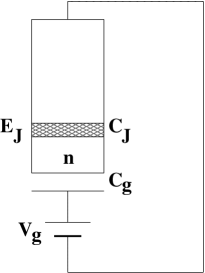
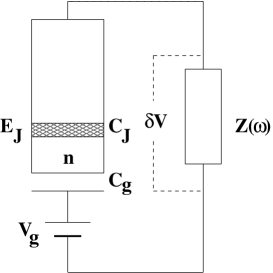
Figure 1: a) A Josephson charge qubit in its simplest design formed by a superconducting single-charge box. b) A qubit with the electromagnetic environment represented by the impedance $Z(\omega)$.

2.1 Josephson qubits, the Hamiltonian and the dissipation

Fig. 1 shows an example of a ‘Josephson charge qubit’ built from superconducting tunnel junctions. All Josephson qubits have in common that they are nanometer-size electronic elements embedded into and manipulated by electrical circuits. The electromagnetic environment, which can not be avoided if we want to control the qubit, leads also to dissipation. This environment plays a crucial role in many contexts, e.g., the physics of the Coulomb blockade in tunnel junctions, for which the appropriate theory is reviewed by Ingold_Nazarov. In the spirit of this analysis we will analyze the effects of the environment on Josephson qubits.

We first consider a superconducting single-charge box shown in Fig. 1a in the absence of dissipation. We further choose parameters such that single-electron tunneling is suppressed and only Cooper-pair charges tunnel across the junction. This situation is realized if the superconducting gap $\Delta$ is larger than the charging energy scale $E_{\rm C}$ (defined below) and the temperature $k_{\rm B}T$. In this case superconducting charge box is described by the Hamiltonian

$$H_{\rm box}=4E_{\rm C}\left(n-\frac{Q_{\rm g}}{2e}\right)^{2}-E_{\rm J}\cos\theta\ .$$ (5)

Here n is the operator counting the number of excess Cooper pairs on the island relative to a neutral reference state. It is conjugate to $\theta$, the phase difference of the superconducting order parameter across the junction. Charge quantization requires that physical quantities are $2\pi$-periodic functions of $\theta$, for instance $e^{i\theta}$, with $e^{i\theta}|n\rangle=|n+1\rangle$. The ‘gate charge’ $Q_{\rm g}\equiv C_{\rm g}V_{\rm g}$ is controlled by the gate voltage, and $E_{\rm C}\equiv e^{2}/2(C_{\rm J}+C_{\rm g})$, which depends on the junction and gate capacitances, is the single-electron charging energy scale. Interactions with charges in the substrate induced by stray capacitances, leads to additional contributions to the gate charge.

Next we account for the dissipation due to electromagnetic fluctuations. They can be modeled by an effective impedance $Z(\omega)$, placed in series with the voltage source (see Fig. 1b) and producing a fluctuating voltage. The sum $V_{\rm g}+\delta V(t)$ couples to the charge in the circuit. For an impedance with open leads the Johnson-Nyquist expression relates the voltage fluctuations between its terminals to $Z(\omega)$. In the present case the impedance is embedded in a circuit, which further modifies the spectrum of voltage fluctuations. Neglecting for a moment the Josephson tunneling (i.e., treating the Josephson junction as a capacitor) we obtain from the fluctuation-dissipation theorem (FDT)

$$S_{V}(\omega)\equiv\frac{1}{2}\int dt\,e^{i\omega t}\langle\left\{\delta V(t),\delta V(0)\right\}\rangle={\rm Re}Z_{\rm t}(\omega)\,\hbar\omega\coth\frac{\hbar\omega}{2k_{\rm B}T}\ .$$ (6)

Here $Z_{\rm t}(\omega)\equiv\left[-i\omega C_{\rm t}+Z^{-1}(\omega)\right]^{-1}$ and $C_{\rm t}^{-1}=C_{\rm J}^{-1}+C_{\rm g}^{-1}$ are the total impedance and capacitance as seen from the terminals of $Z(\omega)$, respectively.

For many purposes it is sufficient to characterize the environment by its noise spectrum and the corresponding response function. In general one should take into account that the environment itself is also a quantum system with many degrees of freedom. As argued before [Caldeira and Leggett (1983)], in a generic setting one can think of a linear environment as of a large set of harmonic oscillators, each of which interacts weakly with the system of interest. I.e., $H_{\rm bath}\equiv\sum_{a}\left[\frac{p_{a}^{2}}{2m_{a}}+\frac{m_{a}\omega_{a}^{2}}{2}x_{a}^{2}\right]$, and the qubit is coupled to the fluctuation variable $\delta V=\sum_{a}\lambda_{a}x_{a}$. The Johnson-Nyquist relation (6) is reproduced if one chooses the bath ‘spectral density’ as $J_{V}(\omega)\equiv{\pi\over 2}\sum_{a}\frac{\lambda_{a}^{2}}{m_{a}\omega_{a}}\delta(\omega-\omega_{a})=\omega\,{\rm Re}Z_{\rm t}(\omega)$. The Hamiltonian of the whole system then reads

$$H=H_{\rm box}-2en{C_{\rm t}\over C_{\rm J}}\,\delta V+H_{\rm bath}+\frac{1}{2\tilde{C}_{\rm t}}\left(2en{C_{\rm t}\over C_{\rm J}}\right)^{2}\ .$$ (7)

The last ‘counter-term’ is introduced to cancel the renormalization of the qubit’s charging energy by the environment. The capacitance $\tilde{C}_{\rm t}$ is defined by $\int_{0}^{\infty}d\omega\,J_{V}(\omega)/\omega\equiv\pi/(2\tilde{C}_{\rm t})$. Because of the analytic properties of response functions it also equals $\tilde{C}_{\rm t}=C_{\rm t}+\lim_{\omega\to\infty}i/(\omega Z(\omega))$. For a pure resistor $Z(\omega)=R$ it reduces to $C_{\rm t}$. The last three terms in (7) can be lumped as

$$H=H_{\rm box}+\sum_{a}\left[\frac{p_{a}^{2}}{2m_{a}}+\frac{m_{a}\omega_{a}^{2}}{2}\left(x_{a}-\frac{\lambda_{a}}{m_{a}\omega_{a}^{2}}\,2en\frac{C_{\rm t}}{C_{\rm J}}\right)^{2}\right]\,.$$

2.2 Reduction to a two-level system

If we bias the superconducting charge box near a degeneracy point of the charging energy, e.g. at a voltage close to $e/C_{\rm t}$, and choose all other parameters (temperature, frequency and strength of control pulses) appropriate, only two charge states play a role, $\left|n=0\right\rangle$ and $\left|n=1\right\rangle$, which we denote as $\left|\uparrow\right\rangle$ and $\left|\downarrow\right\rangle$, respectively. The leakage to higher charge states can be kept at a low level [Fazio et al. (1999)]. In spin notation, the number operator becomes $n=\frac{1}{2}(1-\sigma_{z})$, while $\cos\theta=\frac{1}{2}\sigma_{x}$, and the effective spin Hamiltonian reads

$$H=-\frac{1}{2}B_{z}(V_{\rm g})\;\sigma_{z}-\frac{1}{2}B_{x}\;\sigma_{x}-\frac{1}{2}X\;\sigma_{z}+H_{\rm bath}\ ,$$ (8)

where $X=-\frac{C_{\rm t}}{C_{\rm J}}\,2e\delta V\,$, $B_{x}=E_{\rm J}$, and

$$B_{z}=\frac{2e}{C_{\rm J}+C_{\rm g}}(e-C_{\rm g}V_{\rm g})=4E_{\rm C}\left(1-\frac{Q_{\rm g}}{e}\right)\ .$$ (9)

The spectral density of the fluctuating field $X$ is related to the power spectrum of voltage fluctuations by

$$S_{X}(\omega)=\frac{1}{2}\left(\left\langle X^{2}_{\omega}\right\rangle+\left\langle X^{2}_{-\omega}\right\rangle\right)=\left(2e\,\frac{C_{\rm t}}{C_{\rm J}}\right)^{2}\,S_{V}(\omega)\ .$$ (10)

Here we defined $\left\langle X^{2}_{\omega}\right\rangle\equiv\int dt\,e^{i\omega t}\left\langle X(t)X(0)\right\rangle$. For the calculation of many properties of the two-level system the knowledge of the symmetrized noise correlator, $S_{X}$, is sufficient. In general, however, the anti-symmetric part $A_{X}(\omega)\equiv\frac{1}{2}\,\langle\left[X(t),X(0)\right]\rangle_{\omega}$ is needed as well. It is related to the response function of the bath $\chi(t)=(i/\hbar)\theta(t)\langle[X(t),X(0)]\rangle$, which describes the reaction of the bath to a perturbing force. Namely, if a perturbation $H_{\rm p}=-fX$ is added to the Hamiltonian the bath responds as $\langle X\rangle_{\omega}=\chi(\omega)f(\omega)$. The function $A_{X}(\omega)$ is related to the imaginary part of the response function, $A_{X}(\omega)=\hbar\chi^{\prime\prime}(\omega)$, and in equilibrium the FDT fixes $S_{X}(\omega)=A_{X}(\omega)\coth(\hbar\omega/2k_{\rm B}T)$.

To simplify the comparison with the literature on the Caldeira-Leggett model we include the prefactor in (10) into the definition of the spectral density, $J_{X}(\omega)\equiv(2eC_{\rm t}/C_{\rm J})^{2}J_{V}(\omega)=\chi^{\prime\prime}(\omega)$. The generic low-frequency behavior is a power-law, $J_{X}(\omega)=2\pi\hbar\alpha\omega_{0}^{1-s}\omega^{s}$, where $\omega_{0}$ is a frequency scale and $\alpha$ the dimensionless strength of the dissipation. Of particular interest is the Ohmic case ($s=1$), obtained if $Z(\omega)=R$ and, hence, ${\rm Re}\,Z_{\rm t}(\omega)\approx R$, for $\omega\ll(RC_{\rm t})^{-1}$. In this case we have $J_{X}=2\pi\hbar\alpha\omega\,$ and

$$S_{X}(\omega)=2\pi\hbar^{2}\alpha\omega\coth\frac{\hbar\omega}{2k_{\rm B}T}\,,$$ (11)

with

$$\alpha=\frac{R}{R_{\rm Q}}\,\left(\frac{C_{\rm t}}{C_{\rm J}}\right)^{2}\ ,$$ (12)

and $R_{\rm Q}\equiv(2e)^{2}/h$ is the (superconducting) resistance quantum.

3 Dissipative dynamics

3.1 Bloch equations

The dissipative dynamics of spins has been the subject of extensive research in the context of the nuclear magnetic resonance (NMR). One of the main tools in this field are the Bloch equations. These kinetic equations were first formulated, on phenomenological grounds, by Bloch_Initial for the case of nuclei in a magnetic field $\vec{B}=\vec{B}_{\parallel}+\delta\vec{B}_{\perp}(t)$, which is the sum of a strong static field $\vec{B}_{\parallel}$ in the $z$-direction, and a weak, time-dependent, transverse perturbation $\delta\vec{B}_{\perp}(t)$. The latter may be chosen to oscillate in resonance with the Larmor frequency $B_{\parallel}/\hbar$ to induce spin flips. The Bloch equations describe the dynamics of the magnetization in the ‘anisotropic $\tau$-approximation’:

$$\frac{d}{dt}\vec{M}=-\vec{B}\times\vec{M}-\frac{1}{T_{1}}(M_{z}-M_{0})\vec{z}-\frac{1}{T_{2}}(M_{x}\vec{x}+M_{y}\vec{y})\ .$$ (13)

The two relaxation times, $T_{1}$ and $T_{2}$, characterize the relaxation of the longitudinal component of the magnetization $M_{z}$ to $M_{0}$, which is the equilibrium magnetization in the static field $\vec{B}_{\parallel}$, and the transverse components ($M_{x}$, $M_{y}$) to zero, respectively. Eq. (13) describes the evolution of a two-level system in terms of its ‘magnetization’ $\vec{M}\propto\left\langle\vec{\sigma}\right\rangle$, and at the same time it describes the time evolution of the components of its density matrix, related to the magnetization by $\left\langle\sigma_{z}\right\rangle=\rho_{00}-\rho_{11}$ and $\left\langle\sigma_{x}+i\sigma_{y}\right\rangle=\rho_{10}$. Here $0$ and $1$ denote the ground state, $\left|\uparrow_{z}\right\rangle$, and excited state, $\left|\downarrow_{z}\right\rangle$, in the field $B_{\parallel}$, respectively.

Using the normalization, $\mathop{\rm tr}\hat{\rho}=\rho_{00}+\rho_{11}=1$, one can rewrite Eq. (13) as equations of motion for the density matrix:

$$\dot{\rho}_{00} = -\Gamma_{\uparrow}\rho_{00}+\Gamma_{\downarrow}\rho_{11}\ ,$$

$$\dot{\rho}_{11} = \Gamma_{\uparrow}\rho_{00}-\Gamma_{\downarrow}\rho_{11}\ ,$$

$$\dot{\rho}_{01} = -iB_{\parallel}\rho_{01}-\frac{1}{T_{2}}\rho_{01}\ ,$$ (14)

where the excitation rate $\Gamma_{\uparrow}$ and relaxation rate $\Gamma_{\downarrow}$ are related to $T_{1}$ and the equilibrium value $\langle\sigma_{z}\rangle_{0}$ by $1/T_{1}=\Gamma_{\downarrow}+\Gamma_{\uparrow}$ and $\langle\sigma_{z}\rangle_{0}=T_{1}(\Gamma_{\downarrow}-\Gamma_{\uparrow})$.

A series of papers were devoted to the derivation and generalization of the Bloch equations [Wangsness and Bloch (1953), Bloch (1957), Redfield (1957)]. Below we will illustrate the derivation from the model (8) in several limits of the qubit’s dynamics. We can anticipate two different regimes: The Hamiltonian-dominated regime where the dissipative effects are slow compared to the Larmor precession. In this case it is convenient to describe the dynamics in the eigenbasis of the spin’s Hamiltonian. The other, dissipation-dominated regime, arises, when the total magnetic field is weak. Then the dissipation dominates, and the preferred eigenbasis is that of the dissipative part of the Hamiltonian ($\propto\sigma_{z}$).

3.2 Golden Rule and the Bloch equations

In the eigenbasis of the spin (qubit) the Hamiltonian (8) reads

$$H=-\frac{1}{2}\Delta E\;\sigma_{z}-\frac{1}{2}X\,\left(\cos\eta\;\sigma_{z}-\sin\eta\;\sigma_{x}\right)+H_{\rm bath}\ ,$$ (15)

where $\Delta E\equiv\sqrt{B_{z}^{2}+B_{x}^{2}}\,$ and $\,\tan\eta=B_{x}/B_{z}$. We denote the ground and excited states of the free qubit by $\left|0\right\rangle$ and $\left|1\right\rangle$, respectively. The coupling to the bath is a sum of a transverse ($\propto\sin\eta$) and a longitudinal ($\propto\cos\eta$) term. Only the transverse part can cause spin flips. In the weak-noise limit we consider $X$ as a perturbation and apply Fermi’s golden rule to obtain the relaxation rate, $\Gamma_{\downarrow}=\Gamma_{\left|1\right\rangle\to\left|0\right\rangle}$, and excitation rate, $\Gamma_{\uparrow}=\Gamma_{\left|0\right\rangle\to\left|1\right\rangle}$. E.g., for $\Gamma_{\downarrow}$ we obtain

$$\Gamma_{\downarrow} = \frac{2\pi}{\hbar}\;\frac{\sin^{2}\eta}{4}\;\sum_{i,f}\rho_{i}\;|\left\langle i\right|X\left|f\right\rangle|^{2}\;\delta(E_{i}+\Delta E-E_{f})$$ (16)

$$= \frac{2\pi}{\hbar}\;\frac{\sin^{2}\eta}{4}\;\sum_{i,f}\rho_{i}\;\left\langle i\right|X\left|f\right\rangle\left\langle f\right|X\left|i\right\rangle\;\frac{1}{2\pi\hbar}\int dt\;e^{i\frac{t}{\hbar}\;(E_{i}+\Delta E-E_{f})}$$

$$= \frac{\sin^{2}\eta}{4\hbar^{2}}\;\int dt\;\sum_{i}\rho_{i}\;\left\langle i\right|X(t)X\left|i\right\rangle\;e^{i\frac{t}{\hbar}\;\Delta E}$$

$$= \frac{\sin^{2}\eta}{4\hbar^{2}}\;\langle X^{2}_{\omega=\Delta E/\hbar}\rangle\ .$$

Here $\left|i\right\rangle$ and $\left|f\right\rangle$ are the initial and the final states of the bath and $\rho_{i}$ is the probability for the bath to be initially in the state $\left|i\right\rangle$. Similarly, we obtain

$$\Gamma_{\uparrow}=\frac{\sin^{2}\eta}{4\hbar^{2}}\;\langle X^{2}_{\omega=-\Delta E/\hbar}\rangle\ .$$ (17)

For the relaxation time we thus find

$$\frac{1}{T_{1}}=\Gamma_{\downarrow}+\Gamma_{\uparrow}=\frac{\sin^{2}\eta}{2\hbar^{2}}\;S_{X}(\omega=\Delta E/\hbar)\ ,$$ (18)

and for the equilibrium magnetization

$$\langle\sigma_{z}\rangle_{0}=\frac{\Gamma_{\downarrow}-\Gamma_{\uparrow}}{\Gamma_{\downarrow}+\Gamma_{\uparrow}}=\frac{A_{X}(\omega=\Delta E/\hbar)}{S_{X}(\omega=\Delta E/\hbar)}=\tanh\frac{\Delta E}{2k_{\rm B}T}\ .$$ (19)

The golden rule can also be used to evaluate the dephasing time. Here we skip the derivation since it will be performed in Section 3.5 in the framework of the Bloch-Redfield approximation. The result is

$$T_{2}^{-1}=\frac{1}{2}T_{1}^{-1}+\frac{1}{2\hbar^{2}}\cos^{2}\eta\,S_{X}(\omega=0)\,.$$ (20)

Note that the first term $\propto S(\omega=\Delta E/\hbar)$ in Eq. (20) is the result of the transverse noise, which involves transitions between the qubit’s states with the energy change of $\Delta E$. The second term $\propto S(\omega=0)$ is associated with the longitudinal noise, which does not flip the spin and therefore involves only transitions in the bath without energy transfer. It produces a random contribution to energy differences, and hence to the accumulated phase difference. This contribution to the dephasing rate is sometimes called the “pure-dephasing” rate, $1/T_{2}^{*}$, so that $T_{2}^{-1}=\frac{1}{2}\,T_{1}^{-1}+(T_{2}^{*})^{-1}$.

3.3 Diagrammatic technique

Figure 2: Diagrammatic representation of the propagator $\Pi$.

We proceed with a systematic perturbative analysis of the time evolution of the qubit’s density matrix based on the Keldysh diagrammatic technique. We derive the Bloch equations and the corresponding dissipative times within the so-called Bloch-Redfield approximation, which may be thought of as a generalized golden rule. The systematic extensions allow us to analyze effects of higher orders in the noise and of long-time noise correlations. We will also determine the limits of applicability of the Bloch equations.

First we briefly sketch the derivation of the master equation for the evolution of the density matrix, based on the formalism developed by Schoeller_PRB. With the interaction Hamiltonian

$$H_{\rm int}=-\frac{1}{2}\,X\left(\cos\eta\;\sigma_{z}-\sin\eta\;\sigma_{x}\right)$$ (21)

the time evolution of the density matrix in the interaction representation follows from

$$\rho(t)=Te^{-\frac{i}{\hbar}\int\limits_{t_{0}}^{t}H_{\rm int}(t^{\prime})dt^{\prime}}\rho(t_{0})\;\tilde{T}e^{\frac{i}{\hbar}\int\limits_{t_{0}}^{t}H_{\rm int}(t^{\prime})dt^{\prime}}\ .$$ (22)

Assuming that initially, at $t=t_{0}$, the density matrix is factorized, $\hat{\rho}(t_{0})=\rho_{s}(t_{0})\otimes\rho_{\rm bath}$, we trace Eq. (22) over the bath degrees of freedom and obtain a perturbative expansion for the propagator $\Pi$ of the spin’s density matrix $\rho_{\rm s}(t)=\Pi(t,t_{0})\rho_{\rm s}(t_{0})$. On one hand, the assumption of a factorized initial condition allows us to introduce the characteristics of the bath, e.g. its temperature. On the other hand, it may introduce artifacts. In general we find for $\rho_{\rm s}$ a non-Markovian (nonlocal in time) evolution equation such that the behavior at a time $t$ involves knowledge of $\rho_{\rm s}$ at earlier times. However, often the kernel of this integral equation has a limited range $\tau_{\rm c}$ and does not depend on the initial spin state. Then the simple assumption about the initial density matrix should not influence the long-time evolution.

By tracing out the bath degrees of freedom in Eq. (22) and expanding in $H_{\rm int}$, one obtains a perturbative series. A typical contribution to $\Pi$ is shown in Fig. 2. The upper line contains vertices (the terms $H_{\rm int}$) from the first, time-ordered exponent in Eq. (22), and the lower one contains vertices from the other, inversely time-ordered exponent. As one can see from Eq. (21), each vertex in the diagrams contains one bath operator $X$. The emerging averages of their products reduce, due to Wick’s theorem, in a standard way to pairwise averages, which are shown by the thin lines in the figure. In Fig. 3a the diagrammatic rules for the thin lines are sketched. The horizontal solid lines (see Fig. 3b) describe explicitly the evolution of the spin degree of freedom, each line corresponding to (a $2\times 2$ operator) $\exp[\pm iH_{\rm s}(t-t^{\prime})]$ with different signs for the upper and lower lines.

Figure 3: Basic elements of the diagrammatic technique.

The propagator $\Pi$ satisfies the Dyson equation shown in Fig. 4. Taking the time derivative one arrives at the master (kinetic) equation

$$\frac{d}{dt}\rho_{\rm s}(t) = \frac{i}{\hbar}\left[\rho_{\rm s}(t),H_{\rm s}\right]+\int\limits_{0}^{t}dt^{\prime}\;\Sigma(t-t^{\prime})\;\rho_{\rm s}(t^{\prime})$$ (23)

$$= L_{\rm s}\rho_{\rm s}(t)+\int\limits_{0}^{t}dt^{\prime}\;\Sigma(t-t^{\prime})\;\rho_{\rm s}(t^{\prime})\ .$$

We introduced the Liouville operator $L_{\rm s}\rho_{\rm s}\equiv(i/\hbar)\,\left[\rho_{\rm s},H_{\rm s}\right]$. The self-energy $\Sigma$ is defined as the sum of all irreducible diagrams, i.e., diagrams that can not be divided by cutting the upper and lower solid lines at the same time (see an example in Fig. 5). It is an operator in the space of density matrices, i.e., a tensor of rank four. We denote its components by $\Sigma_{nn^{\prime}\leftarrow mm^{\prime}}$, implying the following action on density matrices: $\displaystyle(\Sigma\rho_{\rm s})_{nn^{\prime}}=\sum_{mm^{\prime}}\Sigma_{nn^{\prime}\leftarrow mm^{\prime}}\,(\rho_{\rm s})_{mm^{\prime}}$.

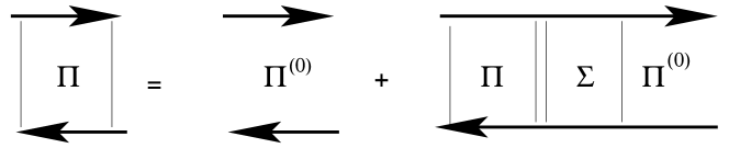
Figure 4: The Dyson equation for the propagator $\Pi$.

Figure 5: A (second-order) contribution to $\Sigma_{nn^{\prime}\leftarrow mm^{\prime}}(t-t^{\prime})$.

3.4 Bloch-Redfield and the rotating-wave approximations

Under certain conditions Eq. (23) may be approximated by a simpler equation which is local in time. Indeed, the self-energy (which in lowest order is proportional to the noise correlator) in the last term on the right hand side decays on time differences $t-t^{\prime}$ of the order of $\tau_{\rm c}$. If this time is much shorter than the dissipative dephasing and relaxation times we may replace the density matrix in the integral from $t^{\prime}$ to $t$ by the leading term

$$\rho_{\rm s}(t^{\prime})\approx e^{-L_{\rm s}(t-t^{\prime})}\;\rho_{\rm s}(t)\ ,$$ (24)

and obtain a Markovian evolution equation

$$\frac{d}{dt}\rho_{\rm s}(t)=L_{\rm s}\,\rho_{\rm s}(t)+\hat{\Gamma}\,\rho_{\rm s}(t)\,.$$ (25)

It involves the ‘Bloch-Redfield tensor’

$$\hat{\Gamma}\equiv\int\limits_{-\infty}^{\infty}dt\;\hat{\Sigma}(t)\;e^{-L_{\rm s}t}\,.$$ (26)

To simplify the Fourier analysis here and in the following, the definition of the self-energy is extended to negative times with $\hat{\Sigma}(t<0)=0$. In the eigenbasis of $H_{\rm s}$ the Liouvillian $L_{\rm s}$ is diagonal, $[L_{\rm s}]_{mm^{\prime}\leftarrow mm^{\prime}}=i(E_{m}-E_{m^{\prime}})\hbar$, and the components of the Bloch-Redfield tensor are related to the self-energy: $\Gamma_{nn^{\prime}\leftarrow mm^{\prime}}=\Sigma_{nn^{\prime}\leftarrow mm^{\prime}}(\hbar\omega=E_{m}-E_{m^{\prime}})$.

To verify the validity of the Bloch-Redfield approximation one should check whether the dissipative times $T_{1}$, $T_{2}$ in the resulting Bloch equations are indeed much longer than the correlation time $\tau_{\rm c}$ of the integrand in Eq. (26) [more precisely, whether the integral is dominated by times shorter than $T_{1}$ and $T_{2}$]. 

In certain cases the equations of motion can be simplified further by employing the rotating-wave approximation (RWA). It is based on the following considerations: if the dissipation is weak and the dynamics of the components of the density matrix close to the unperturbed dynamics, the spectral weight of $\rho_{nn^{\prime}}(t)$ is located in the vicinity of $\omega=(E_{n}-E_{n^{\prime}})/\hbar\equiv\omega_{nn^{\prime}}^{0}$. The rhs of the $nn^{\prime}$-component of the equation of motion (25) contains contributions from all components $mm^{\prime}$ of the density matrix. However, if $\omega_{mm^{\prime}}^{0}\neq\omega_{nn^{\prime}}^{0}$ this contribution averages out fast (on the time scale $\hbar/(\omega_{mm^{\prime}}^{0}-\omega_{nn^{\prime}}^{0})$) and can be neglected. I.e., one truncates the terms $\Gamma_{nn^{\prime}\leftarrow mm^{\prime}}\rho_{mm^{\prime}}$ on the rhs of the equation of motion: for the diagonal elements $\rho_{nn}$ one keeps only the diagonal entries, while for the off-diagonal elements, e.g. $\rho_{01}$, one keeps only the contribution from the same entry, e.g. the component $\Gamma_{01\leftarrow 01}$. The latter are, in general, complex numbers, with a real part describing dephasing and an imaginary part corresponding to a renormalization of the energy.

If the system is subject to a strong pulse, Eq. (25) may not be sufficient. Typically the initial evolution for a certain period of time $\sim\tau_{\rm c}$ needs to be described by other methods. However, the following time evolution is governed by (25). We will discuss examples in Section 5.3. Another situation, where Eq. (25) may be not sufficient is the case where the noise shows long-range correlations (cf. the discussion of the 1/f noise in Section 5.1).

3.5 $T_{1}$ and $T_{2}$

As an example and demonstration of the diagrammatic expansion we rederive the expressions for $T_{1}$ and $T_{2}$, obtained before by golden rule arguments in Section 3.2. The lowest-order contributions to the rate $\Gamma_{00\leftarrow 11}=\Gamma_{\downarrow}$ are shown in Fig. 6.

Figure 6: Leading-order contributions to $\Gamma_{00\leftarrow 11}$.

We obtain

$$\Sigma_{00\leftarrow 11}(t-t^{\prime})=\frac{\sin^{2}\eta}{4\hbar^{2}}\,\left[\langle X(t)X(t^{\prime})\rangle e^{\frac{i}{\hbar}\Delta E(t-t^{\prime})}+c.c.\right]\ ,$$ (27)

and thus, from Eq. (26) and the fact that ${(L_{\rm s})}_{11\leftarrow 11}=0$, we get

$$\Gamma_{\downarrow}=\Gamma_{00\leftarrow 11}=\Sigma_{00\leftarrow 11}(\omega=0)=$$

$${\rm Re}\left[-\frac{i\sin^{2}\eta}{2\hbar^{2}}\int\frac{d\omega^{\prime}}{2\pi}\;\frac{\langle X^{2}_{\omega^{\prime}}\rangle}{\omega^{\prime}-(\Delta E/\hbar)-i0}\right]=$$

$$\frac{\sin^{2}\eta}{4\hbar^{2}}\;\langle X^{2}_{\omega=\Delta E/\hbar}\rangle\ .$$ (28)

In the same way one can obtain the excitation rate $\Gamma_{11\leftarrow 00}\equiv\Gamma_{\uparrow}$, and hence $T_{1}$, as well as the rates $\Gamma_{00\leftarrow 00}=-\Gamma_{11\leftarrow 00}$ and $\Gamma_{11\leftarrow 11}=-\Gamma_{00\leftarrow 11}$.

As for the dephasing time $T_{2}$, the relevant lowest-order contributions to $\Gamma_{01\leftarrow 01}$ are shown in Fig. 7. The upper row of the diagrams shows the contribution of the transverse fluctuations $\Sigma_{01\leftarrow 01}^{\perp}$ and the lower row shows that of the longitudinal fluctuations $\Sigma_{01\leftarrow 01}^{\parallel}$, so that $\Sigma_{01\leftarrow 01}=\Sigma_{01\leftarrow 01}^{\perp}+\Sigma_{01\leftarrow 01}^{\parallel}$.

Figure 7: Leading-order contributions to $\Gamma_{01\leftarrow 01}$.

The transverse and longitudinal contributions give:

$$\Sigma_{01\leftarrow 01}^{\perp}(t-t^{\prime})=-\frac{\sin^{2}\eta}{2\hbar^{2}}\,S(t-t^{\prime})\ ,$$ (29)

$$\Sigma_{01\leftarrow 01}^{\parallel}(t-t^{\prime})=-\frac{\cos^{2}\eta}{\hbar^{2}}\,S(t-t^{\prime})\,e^{\frac{i}{\hbar}\,\Delta E(t-t^{\prime})}\ .$$ (30)

Noting that ${(L_{\rm s})}_{01\leftarrow 01}=i\Delta E/\hbar$ we obtain from Eq. (26)

$$\Gamma_{01\leftarrow 01}^{\perp} = \frac{i\sin^{2}\eta}{2\hbar^{2}}\int\frac{d\omega}{2\pi}\;\frac{S_{X}(\omega)}{\omega+(\Delta E/\hbar)-i0}\ ,$$ (31)

$$\Gamma_{01\leftarrow 01}^{\parallel} = \frac{i\cos^{2}\eta}{\hbar^{2}}\int\frac{d\omega}{2\pi}\;\frac{S_{X}(\omega)}{\omega-i0}\ ,$$ (32)

and $\Gamma_{01\leftarrow 01}=\Gamma_{01\leftarrow 01}^{\perp}+\Gamma_{01\leftarrow 01}^{\parallel}$. The real part of these entries of the Redfield tensor, ${\rm Re}\,\Gamma_{01\leftarrow 01}=-T_{2}^{-1}$, reproduces the dephasing rate (20).

3.6 Energy renormalization

The analysis of the preceding subsection also shows that the qubit’s level splitting is renormalized by the bath. This effect is the analogue of the Lamb shift, i.e. the renormalization of the level splitting in atoms due to the coupling to the electromagnetic radiation. As can be seen from Eq. (25) an imaginary part of $\Gamma_{01\leftarrow 01}$ gives rise to such a renormalization. Only the transverse noise contributes to this renormalization. From Eq. (31) we obtain

$${\rm Im}\,\Gamma_{01\to 01}=-\frac{\sin^{2}\eta}{2\hbar^{2}}\;{\rm P}\int\frac{d\omega}{2\pi}\;\frac{S_{X}(\omega)}{\omega-(\Delta E/\hbar)}\ .$$ (33)

As an example we consider an oscillator bath with Ohmic spectral density up to a high-frequency cut-off, $J(\omega)=2\pi\alpha\hbar\omega\Theta(\omega_{c}-\omega)$, at low temperature $k_{\rm B}T\ll\Delta E$ where $S(\Delta E)=J(\Delta E)\coth\frac{\Delta E}{2k_{\rm B}T}\approx J(\Delta E)$, which is coupled purely transversely, $\eta=\pi/2$. Then the integral in (33) is dominated by high frequencies $\hbar\omega>\Delta E$ and gives the following correction to the energy splitting: $\Delta E\rightarrow\Delta E(1-\alpha\ln(\hbar\omega_{c}/\Delta E))$. This result indicates that the small parameter of the perturbative expansion is $\alpha\ln(\hbar\omega_{c}/\Delta E)$, rather than $\alpha$. Also for general bath spectra the high-frequency part of the spectrum typically leads to a renormalized Hamiltonian. The effect can be calculated perturbatively as shown above or in the frame of a renormalization-group approach, which accounts for all orders in the small parameter. It turns out that in such a situation only the component of the field perpendicular to the direction of the fluctuating field is affected by the renormalization [Leggett et al. (1987), Weiss (1999)].

The effect of low-frequency fluctuations can be treated adiabatically: They do not induce transitions between the qubit states, but they change their energy splitting since the fluctuations of the transverse component of the ‘magnetic field’ $X^{\perp}$ increase the average magnitude of the field.

Even if the bare Hamiltonian is time-dependent the contribution of the high-frequency modes ($\hbar\omega\gg\Delta E$) of the environment can be absorbed in a renormalization of the Hamiltonian. In contrast, the analysis of the effect of low-frequency modes depends on further details.

4 Applications

4.1 Ohmic dissipation in real devices

For an Ohmic environment we obtain from Eqs. (18) and (20)

$$T_{1}^{-1} = \pi\alpha\;\sin^{2}\eta\;\frac{\Delta E}{\hbar}\coth\displaystyle\frac{\Delta E}{2k_{\rm B}T}\;,$$ (34)

$$T_{2}^{-1} = \frac{1}{2}\;T_{1}^{-1}+\pi\alpha\;\cos^{2}\eta\;\frac{2k_{\rm B}T}{\hbar}\;.$$ (35)

For the charge qubit the coupling constant $\alpha$ is given by Eq. (12). The typical impedance of the control line is $R\approx 50~{}\Omega$. Since $R_{\rm Q}\approx 6.5~{}{\rm k}\Omega$ we obtain $\alpha\approx 10^{-2}(C_{\rm t}/C_{\rm J})^{2}$. With the typical values of the capacitances $C_{\rm J}\approx 10^{-16}{\rm F}$ and $C_{\rm g}\approx 10^{-18}{\rm F}$ their ratio can be made as small as $10^{-2}$. Thus $\alpha$ can be as small as $10^{-6}$. At temperature $T\approx 10$ mK and for $\Delta E/k_{\rm B}\approx 1$ K, we estimate the pure dephasing time $T_{2}^{*}\approx 100~{}\mu$s (for $\eta=0$) and the relaxation time $T_{1}\approx 1~{}\mu$s (for $\eta=\pi/2$). In recent experiments [Vion et al. (2002), Chiorescu et al. (2003)] similar values of $T_{1}$ have been observed, however $T_{2}$ was much shorter. This has been attributed to the contribution of the $1/f$ noise (i.e. dominated by low-frequencies), which we discuss below.

4.2 Validity of the Bloch-Redfield approximation in the Ohmic case

As mentioned above, after having solved the Bloch equations one should verify the validity of the Bloch-Redfield approximation by checking the self-consistency. Let us consider the example of a weakly coupled Ohmic environment, $\alpha\ll 1$. The Bloch-Redfield approximation is justified provided the integral in Eq. (26) converges on a time scale short compared to the appropriate dissipative time $T_{1}$ or $T_{2}$.
(i) For the evaluation of $T_{1}^{-1}\propto S(\Delta E/\hbar)\sin^{2}\eta$ consistency requires that the noise power in the vicinity of $\omega=\Delta E/\hbar$ varies smoothly on the scale $T_{1}^{-1}$. For the Ohmic bath this condition is always satisfied: in the limit $\Delta E\gg k_{\rm B}T$ it reduces to $\alpha\Delta E\ll\Delta E$ and in the opposite limit to $\alpha T\ll T$.
(ii) For the evaluation of $T_{2}^{-1}=\frac{1}{2}T_{1}^{-1}+(T_{2}^{*})^{-1}\propto\frac{1}{2}S(\Delta E)\sin^{2}\eta+S(0)\cos^{2}\eta$ the condition may differ only if the rate is dominated by the second term, $T_{2}^{*}$. Then the condition is that the noise power varies weakly on the scale of $(T_{2}^{*})^{-1}\sim\alpha T(k_{\rm B}/\hbar)\ll T(k_{\rm B}/\hbar)$ around zero frequency, which is always true.

We conclude that for $\alpha\ll 1$ the Bloch-Redfield approximation is valid.

4.3 Environment-dominated dynamics

Consider a Hamiltonian with purely transverse coupling, $\eta=\pi/2$:

$$H=-\frac{1}{2}\Delta E\;\sigma_{z}+\frac{1}{2}X\;\sigma_{x}+H_{\rm bath}\ .$$ (36)

For this model the Bloch-Redfield tensor becomes:

$$\frac{d}{dt}\left(\begin{array}[]{c}\rho_{00}\\ \rho_{11}\\ \rho_{01}\\ \rho_{10}\\ \end{array}\right)=\left(\begin{array}[]{cccc}-\Gamma_{\uparrow}&\Gamma_{\downarrow}&0&0\\ \Gamma_{\uparrow}&-\Gamma_{\downarrow}&0&0\\ 0&0&i\Delta E-\Gamma_{\varphi}&\Gamma_{\varphi}^{*}\\ 0&0&\Gamma_{\varphi}&-i\Delta E-\Gamma_{\varphi}^{*}\\ \end{array}\right)\left(\begin{array}[]{c}\rho_{00}\\ \rho_{11}\\ \rho_{01}\\ \rho_{10}\\ \end{array}\right)\ .$$ (37)

Here $\Gamma_{\varphi}\equiv-\Gamma_{01\leftarrow 01}$. If the two-level system is almost degenerate, $\Delta E\ll\hbar\Gamma_{\varphi}$, the RWA is not valid, and one can not neglect the off-diagonal entries (obtained from diagrams similar to those in Fig. 6). Notice that the degeneracy condition, $\Delta E\ll\Gamma_{\varphi}$, may still be consistent with the validity condition of the Bloch-Redfield approximation, $1/\tau_{\rm c}\gg\Gamma_{\varphi}$. For instance, for an Ohmic bath in the weak-coupling limit, $\alpha\ll 1$, one finds $1/\tau_{\rm c}\sim(k_{\rm B}/\hbar)T\gg\alpha(k_{\rm B}/\hbar)T\sim\Gamma_{\varphi}$ (the latter equality is valid provided $\Delta E\ll k_{\rm B}T$).

In this regime, $\Delta E\ll\hbar\Gamma_{\varphi}$, Eq. (37) has a very slowly decaying eigenmode, with $\hat{\rho}\propto\hat{\sigma}_{x}$, with the relaxation rate $(\Delta E)^{2}/2\Gamma_{\varphi}$ ($\Gamma_{\varphi}$ is almost real). This phenomenon is called the quantum Zeno effect [Misra and Sudarshan (1977)]. The environment “observes” $\sigma_{x}$ and prevents it from relaxing. The effect has the remarkable property that the stronger the dephasing, $\Gamma_{\varphi}$, the slower the relaxation.

In general, in the dissipation-dominated regime it is more convenient to treat the spin Hamiltonian as a perturbation on top of the dissipative dynamics.

4.4 Time-dependent driving: Rabi oscillations

For a general time-dependent magnetic field $\vec{B}(t)$ the description of the dissipative dynamics is more complicated. Here we discuss an example for which the Bloch-Redfield approximation does not apply in the laboratory frame but can be used in the rotating frame (or, equivalently, in the interaction representation).

Consider a situation with the purely longitudinal coupling,

$$H=-\frac{1}{2}\Delta E\;\sigma_{z}-\frac{1}{2}X\;\sigma_{z}+H_{\rm bath}\ ,$$ (38)

for which Eqs. (18) and (20) give $\,T_{1}^{-1}=0$ and $\,T_{2}^{-1}=(1/2\hbar^{2})\,S_{X}(\omega=0)$. Let us now apply a resonant transverse driving field:

$$H=-\frac{1}{2}\Delta E\;\sigma_{z}-\frac{1}{2}\Omega_{\rm R}\;(\cos\omega t\,\sigma_{x}-\sin\omega t\,\sigma_{y})-\frac{1}{2}X\;\sigma_{z}+H_{\rm bath}\,.$$ (39)

The subscript R indicates that this field can induce the so-called Rabi oscillations between the levels. As follows from the discussion in Section 3.4, one can still use the Bloch equations as long as the driving is weak enough, $\Omega_{\rm R}\tau_{\rm c}\ll 1$. For a stronger driving these equations may fail. However, the transformation to the rotating frame [$H\to\tilde{H}=\hbar\,\dot{U}U+UHU^{{\dagger}}$, with $U=\exp\left(-i\omega\sigma_{z}\,t/2\right)$ and $\hbar\omega=\Delta E$] makes the Hamiltonian time-independent:

$$H=-\frac{1}{2}\Omega_{\rm R}\;\sigma_{x}-\frac{1}{2}X\;\sigma_{z}+H_{\rm bath}\ .$$ (40)

The first term on the rhs of Eq. (40) induces coherent oscillations in the rotating frame, with the spin performing an oscillatory motion between the up- and down-states. Furthermore, using Eqs. (18) and (20), we find that the relaxation of the $x$-component of the spin in the rotating frame occurs on the time scale $T_{1}^{-1}=(1/2\hbar^{2})\,S_{X}(\omega=\Omega_{\rm R})$, and the decay of the transverse ($y$- and $z$-) components on the time scale $T_{2}^{-1}=1/(2T_{1})$. One may verify that in the weak-driving limit ($\Omega_{\rm R}\tau_{\rm c}\ll 1$) this result in consistent with the standard Bloch equations in the laboratory frame.

We summarize, strong or fast variations of the Hamiltonian (e.g., the field $\vec{B}(t)$) may invalidate the Bloch equations, but in certain situations one may still reduce the problem to another one for which these equation can be applied. The resulting dissipative times $T_{1}$, $T_{2}$ may, however, differ from those in the original Bloch equations.

5 Beyond the Bloch-Redfield (golden-rule) approximation

5.1 1/f noise

Several experiments with Josephson circuits have revealed at low frequencies the presence of $1/f$ noise. While the origin of this noise may be different in different circuits, it appears that in several cases (especially in the charge devices) it derives from “background charge fluctuations”. This noise is usually presented as an effective noise of the gate charge (see Eq.(5)), i.e., $S_{Q_{\rm g}}(\omega)=\alpha_{1/f}e^{2}/|\omega|$. Recent experiments (cf. Nakamura_Echo and references therein) yield at relevant temperatures $\alpha_{1/f}\sim 10^{-7}$–$10^{-6}$. We translate this noise into fluctuations of the effective magnetic field $X$ with

$$S_{X}(\omega)=\frac{E^{2}_{1/f}}{|\omega|}\ ,$$ (41)

and by comparison with Eq. (9) find $E_{1/f}=4E_{\rm C}\sqrt{\alpha_{1/f}}$.

The Bloch-Redfield result (20) predicts a divergent rate $T_{2}^{-1}\to\infty$, unless $\eta=\pi/2$, and clearly fails in this case. This can be attributed to the very slow (logarithmic) time decay of the function $S_{X}(t)$. It is easy, though, to describe the dephasing due to $1/f$ noise rigorously, if it couples purely longitudinally ($\eta=0$) and is Gaussian distributed. Treating $X$ as a classical variable one obtains [Cottet et al. (2001)]

$$\langle\sigma_{+}(t)\rangle\propto\left\langle e^{-\frac{i}{\hbar}\,\int\limits_{0}^{t}dt^{\prime}\,X(t^{\prime})}\right\rangle=e^{-\frac{1}{2\hbar^{2}}\int\limits_{0}^{t}dt^{\prime}\;\int\limits_{0}^{t}dt^{\prime\prime}\langle X(t^{\prime})X(t^{\prime\prime})\rangle}$$

$$=\exp\left({-\frac{1}{2\hbar^{2}}\,\int\frac{d\omega}{2\pi}\,S_{X}(\omega)\,\frac{\sin^{2}(\omega t/2)}{\left(\omega/2\right)^{2}}}\right)\ .$$ (42)

This result coincides with the real part of Eq. (54) obtained in a quantum description. For a regular low-frequency spectrum one may replace the last fraction in (5.1) by $2\pi\delta(\omega)\,t\,$ and obtain the golden-rule result for the dephasing time. For the $1/f$ noise one obtains with logarithmic accuracy [Cottet et al. (2001)]

$$\langle\sigma_{+}(t)\rangle\propto\exp\left(-\frac{E_{1/f}^{2}}{2\pi\hbar^{2}}\,t^{2}\,|\ln t\omega_{\rm ir}|\right)\ ,$$ (43)

where $\omega_{\rm ir}$ is the infrared cutoff frequency for the $1/f$ noise.  From this decay law one can deduce the dephasing time scale,

$$\frac{1}{T_{2}^{*}}\approx\frac{1}{\hbar}\,E_{1/f}\,\sqrt{\frac{1}{2\pi}\ln\frac{E_{1/f}}{\omega_{\rm ir}}}\ .$$ (44)

Using experimental parameters for an estimate one obtains $T_{2}$ in the range from fractions to a few nanoseconds, which is close to the dephasing time observed in the experiments away from the special point $\eta=\pi/2$. We also see that this source of dephasing dominates over the Ohmic noise.

5.2 Contribution of higher orders

In this section we consider a further situation where the lowest-order Bloch equations are not sufficient. The dissipative times (18, 20) in the Bloch equations are dominated by the noise power at specific frequencies ($0$ and $\Delta E/\hbar$). As an example, consider the purely transverse case, $\eta=\pi/2$, where the first-order Bloch-Redfield formulas give $T_{1}^{-1}=2T_{2}^{-1}=\frac{1}{2\hbar^{2}}S_{X}(\omega=\frac{\Delta E}{\hbar})$. In higher orders of the perturbative expansion (cf. Section 3.3) the noise power in other frequency ranges may be involved. If the noise power in these ranges is much stronger, higher-order contributions may compete with the lowest-order. An important example is the case of $1/f$ noise. Here the strong noise at low frequencies contributes in higher order to the dissipative rates.

To illustrate the importance of higher orders, consider the contribution to the second-order self-energy $\Sigma_{01\leftarrow 01}^{(2)}$ shown in Fig. 8a,

Figure 8: Second-order contributions. One can obtain all 16 second-order diagrams by shifting an even number of the vertices in a or b to the lower line.

$$\delta\Sigma_{01\leftarrow 01}^{(2)}=\frac{1}{(2\hbar)^{4}}\int\limits_{t^{\prime}}^{t}d\tau_{1}\int\limits_{t^{\prime}}^{\tau_{1}}d\tau_{2}\,\langle X(t)X(t^{\prime})\rangle\,\langle X(\tau_{1})X(\tau_{2})\rangle e^{i\Delta E(\tau_{1}-\tau_{2})/\hbar}\ .$$ (45)

The factor $e^{\frac{i\Delta E}{\hbar}(\tau_{1}-\tau_{2})}$ is due to the difference in energy of the state on the upper ($\left|0\right\rangle$) and lower ($\left|1\right\rangle$) lines in the time interval between $\tau_{1}$ to $\tau_{2}$. The Fourier transform of Eq. (45) reads

$$\delta\Sigma_{01\leftarrow 01}^{(2)}(\omega)= \frac{-i}{(2\hbar)^{4}}\int\limits_{-\infty}^{\infty}\frac{d\omega_{1}d\omega_{2}}{(2\pi)^{2}}\,\langle X^{2}_{\omega_{1}}\rangle\langle X^{2}_{\omega_{2}}\rangle$$ (46)

$$\times\frac{1}{(\omega-\omega_{1}+i0)^{2}(\omega-\omega_{1}-\omega_{2}+\Delta E/\hbar+i0)}\ .$$

Comparison of Eq. (46) and Fig. 8a elucidates the diagrammatic rules: the bath lines carry the frequencies $\omega_{1}$ and $\omega_{2}$, while pairs of horizontal solid lines contribute factors of the type $1/(\omega-\sum\omega_{n}-i\hat{L}_{\rm s})$, where the summation is over all the bath lines in the interval and the matrix element of $L_{\rm s}$ is determined by the spin states on the upper and lower lines.

There are in total 16 second-order diagrams (see Fig. 8), which contribute to $\Sigma_{01\leftarrow 01}$. They add up to

$$\Sigma_{01\leftarrow 01}^{(2)}(\omega)= \frac{-2i}{(2\hbar)^{4}}\int\limits_{-\infty}^{\infty}\frac{d\omega_{1}d\omega_{2}}{(2\pi)^{2}}\,\left[\frac{1}{\omega-\omega_{1}+i0}+\frac{1}{\omega-\omega_{2}+i0}\right]$$ (47)

$$\times\frac{1}{\omega-\omega_{1}+i0}\left[\frac{\langle X^{2}_{\omega_{1}}\rangle\langle X^{2}_{\omega_{2}}\rangle+\langle X^{2}_{-\omega_{1}}\rangle\langle X^{2}_{-\omega_{2}}\rangle}{\omega-\omega_{1}-\omega_{2}+\Delta E/\hbar+i0}\right.$$

$$\quad\quad\quad\quad+\left.\frac{\langle X^{2}_{\omega_{1}}\rangle\langle X^{2}_{-\omega_{2}}\rangle+\langle X^{2}_{-\omega_{1}}\rangle\langle X^{2}_{\omega_{2}}\rangle}{\omega-\omega_{1}-\omega_{2}-\Delta E/\hbar+i0}\right]\ .$$

We evaluate the behavior of the self-energy in the vicinity of the level splitting, $\Sigma_{01\leftarrow 01}^{(2)}(\omega=-\Delta E/\hbar-\omega^{\prime}+i0)$, where $\omega^{\prime}\ll\Delta E/\hbar$. If the integral (47) is dominated by low frequencies, we obtain:

$${\rm Re}\,\Sigma_{01\leftarrow 01}^{(2)}\Bigl{(}\omega =-\frac{\Delta E}{\hbar}-\omega^{\prime}+i0\Bigr{)}$$ (48)

$$\approx-\frac{1}{8\hbar^{2}\Delta E^{2}}\int\limits_{-\infty}^{\infty}\frac{d\nu}{2\pi}\,\left[\langle X^{2}_{\nu+\omega^{\prime}}\rangle\langle X^{2}_{-\nu}\rangle+\langle X^{2}_{\nu-\omega^{\prime}}\rangle\langle X^{2}_{-\nu}\rangle\right]$$

$$=-\frac{1}{2\hbar^{2}}S_{X_{2}}(\omega^{\prime})\ ,$$

where $S_{X_{2}}$ is the symmetrized correlator of $X_{2}\equiv X^{2}/(2\Delta E)$.

To understand the origin of this result (48) consider the effect of the low-frequency fluctuations (which, we assumed, dominate the dephasing). Starting from the Hamiltonian (15) with the transverse coupling to the noise source, $\eta=\pi/2$, we see that in the adiabatic limit of very slow fluctuations the dynamics reduces to an accumulation of the relative phase between the eigenstates, $\int dt\,\Delta E_{X}(t)/\hbar$, where $\Delta E(X)=\sqrt{\Delta E^{2}+X^{2}}\approx\Delta E+X^{2}/(2\Delta E)$. Thus the problem reduces to the longitudinal case. The calculation above confirms this reduction in the lowest order. More precisely, the second-order contribution to $\Sigma_{01\leftarrow 01}^{(2)}$ for the transversely coupled $X$ coincides with the lowest-order contribution for the longitudinally coupled $X_{2}$.

Notice also that the fluctuating field $X_{2}$ has a nonzero average which provides a (low-frequency contribution to the) renormalization of the level splitting (cf. Section 3.6).

Generally speaking, the result (48) does not allow one to evaluate the dephasing decay law but may be used for qualitative estimates. Consider the example of the $1/f$ noise. In this case the low-frequency behavior of the second-order self-energy is singular and it may compete with the first-order contribution. Higher-order contributions require further analysis (both in the linear transverse and quadratic longitudinal cases). However, one can show that at high enough frequencies the higher-order contributions to $\Sigma$ may be neglected. Thus, the result (48) permits an analysis of the decay law at short times. Extrapolating this law to longer times, one can estimate the typical dephasing time. Qualitatively, this amounts to solving the equation $T_{2}^{-1}\sim-\Sigma_{01\leftarrow 01}^{(2)}(\omega=T_{2}^{-1})$. For $1/f$ spectrum (41) we obtain

$$S_{X_{2}}(\omega)\sim\frac{E_{1/f}^{4}}{(\Delta E)^{2}}\,\frac{1}{|\omega|}\ln\frac{|\omega|}{\omega_{\rm ir}}\ ,$$ (49)

i.e., this noise power is again of the $1/f$ type. This gives the estimate $T_{2}^{-1}\sim(E_{1/f}^{2}/\hbar\Delta E)\ln(E_{1/f}^{2}/\hbar\Delta E\omega_{\rm ir})$.

5.3 Effect of strong pulses

In this section we discuss the effects of a strong pulse of the magnetic field on the dissipative dynamics of the spin. The derivation of the Bloch equations (cf. the discussion in Section 3.4) relied on the slowness of the spin’s dynamics, which may be violated if a strong or a fast-oscillating field is applied. In this case for a period of order $\tau_{\rm c}$ a different description beyond the Bloch-Redfield approximation is needed.

As an example we consider the ‘initial-state preparation’ of a gedanken experiment designed to observe the effects of dephasing on the spin precession. Specifically, we assume that initially the spin was kept at low temperatures in a field $B_{z}\hat{z}$ and has relaxed to the ground state $\left|\uparrow\right\rangle$. Then it is rotated by a strong short $\pi/2$-pulse of the transverse field and starts a free precession in the field $B_{z}\hat{z}$. Under the influence of the bath the relative phase between the spin-up and -down states will not only have a contribution due to the Zeeman splitting, which grows linearly in time, but also a random contribution from the noise, which destroys the phase coherence. For the analysis below we assume the Ohmic spectral density.

The effect of the pulse on the spin’s dynamics, as compared to the Bloch equations, is an additional unitary evolution and dephasing. The former effect is an extra phase acquired by the spin due to the initial polarization of the bath. The latter is the dephasing due to the initial partial disentanglement of the bath and the spin (which amounts to a partial factorization of the initial density matrix), as we illustrate below.

During the relaxation of the spin to the ground state $\left|\uparrow\right\rangle$ the oscillators have also relaxed to the corresponding ground state. I.e., the initial state of the whole system is given by the density matrix $\rho_{0}=\left|\uparrow\right\rangle\left\langle\uparrow\right|\otimes\rho_{\uparrow}$ with $\rho_{\uparrow}\propto\exp(-H_{\uparrow}/k_{\rm B}T)$ and $H_{\uparrow}\equiv H_{\rm bath}-X/2$. In this state the bath operator $X$ provides a finite average field. Its expectation value $\langle X\rangle$ can be calculated as a linear response of the bath to the perturbation $H_{\rm pert}=-fX$ with $f=1/2$, i.e., $\langle X\rangle=\chi(\omega=0)f=\chi^{\prime}(\omega=0)/2$. For an Ohmic spectrum, $\chi^{\prime\prime}(\omega)=2\pi\alpha\hbar\omega$ up to a cutoff $\omega_{\rm c}$, we have $\langle X\rangle=\chi^{\prime}(\omega=0)/2=\int(d\nu\,\chi^{\prime\prime}(\nu))/(2\pi\nu)\sim\alpha\hbar\omega_{\rm c}$. We note that this expectation value depends strongly on the high-frequency cutoff $\omega_{\rm c}$ of the bath spectrum. The field produced by each bath mode averages out after its typical oscillation period; still during a short initial period of length $\sim\omega^{-1}$ it affects the spin dynamics. Depending on the spectral density of the bath, the resulting effect may be dominated by low or high frequencies.

Now we apply a $\pi/2$-pulse to rotate the spin to a position perpendicular to the original state, i.e. into the superposition $(\left|\uparrow\right\rangle+\left|\downarrow\right\rangle)/\sqrt{2}$. If the pulse duration is very short, the state of the bath does not change during the pulse. If the pulse takes a finite time, $\omega_{p}^{-1}$, the bath oscillators partially adjust to the changing spin state. For the high-frequency oscillators, $\omega\gg\omega_{p}$, the spin evolution during the pulse (and afterwards) is adiabatic; they just ‘dress’ the spin, renormalizing its parameters, e.g., its $g$-factor [Shnirman et al. (2002)]. In contrast, the slow oscillators, with $\omega\ll\omega_{p}$, do not have time to react on this short time interval and start to change their states only after the pulse. They react differently for the spin-up and spin-down components, thus contributing to the dephasing. Neglecting, for a qualitative discussion, the oscillators at intermediate frequencies, we find the system in the state $\rho_{0}=\frac{1}{2}\left|\tilde{\uparrow}+\tilde{\downarrow}\right\rangle\left\langle\tilde{\uparrow}+\tilde{\downarrow}\right|\otimes\tilde{\rho}_{\uparrow}$. Here the state $\left|\tilde{\uparrow}\right\rangle$ denotes the state of the dressed spin, i.e. the product state of $\left|\uparrow\right\rangle$ and the equilibrium states of high frequency oscillators under the influence of the spin up (i.e. with the Hamiltonian $H_{\uparrow}$), and similarly for the state $\left|\tilde{\downarrow}\right\rangle$. In short, qualitatively one may think of the system as a dressed spin coupled to a bath with the upper cutoff $\sim\omega_{p}$.

After this initial preparation, the spin starts a precession in the field $B_{z}\hat{z}$. To describe the time evolution in the presence of the bath we split the Hamiltonian (8) as

$$H=-\frac{1}{2}B_{z}\sigma_{z}-\frac{1}{2}X(\sigma_{z}-1)+H_{\uparrow}$$ (50)

and extract explicitly the average $\langle X\rangle$ with the intention to treat the part proportional to $\delta X$ as a perturbation. Hence

$$H=-\frac{1}{2}B_{z}\sigma_{z}-\frac{1}{2}\langle X\rangle(\sigma_{z}-1)-\frac{1}{2}\delta X(\sigma_{z}-1)+H_{\uparrow}\ .$$ (51)

At $t=0$ the spin is subject to the additional field $\langle X\rangle$. We expect that this field relaxes, on the time scale $\omega^{-1}$ for oscillators with frequency $\omega$. Nevertheless, before the field vanishes, it contributes to the phase evolution. Clearly, the spin-up and spin-down states are decoupled, which allows for an exact solution. One may use the so called polaron transformation (cf. LeggettRMP, WeissBook), or calculate the time evolution of the off-diagonal element of the qubit’s density matrix directly:

$$\langle\sigma_{+}(t)\rangle=e^{-\frac{i}{\hbar}B_{z}t}\;{\rm Tr}\,\left[\sigma_{+}\;S(t,0)\;\rho_{0}\;S^{{\dagger}}(t,0)\right]\ ,$$ (52)

where

$$S(t,0)\equiv Te^{\frac{i}{2\hbar}\int\limits_{0}^{t}\delta X(t^{\prime})(\sigma_{z}-1)\,dt^{\prime}}\ .$$ (53)

Obviously, the evolution operators $S$ and $S^{{\dagger}}$ do not flip the spin, while the operator $\sigma_{+}$ in Eq. (52) imposes a selection rule such that the spin is in the state $\left|\downarrow\right\rangle$ on the forward Keldysh contour (i.e., in $S(t,0)$) and in the state $\left|\uparrow\right\rangle$ on the backward contour (i.e., in $S^{{\dagger}}(t,0)$). Since $\left\langle\uparrow\right|\sigma_{z}-1\left|\uparrow\right\rangle=0$ the contribution of the backward contour vanishes. From $\left\langle\downarrow\right|\sigma_{z}-1\left|\downarrow\right\rangle=-2$ we obtain $\langle\sigma_{+}(t)\rangle=P(t)\exp(-iB_{z}t/\hbar)\langle\sigma_{+}(0)\rangle$, where

$$P(t)\equiv\langle T\exp\left(-\frac{i}{\hbar}\int\limits_{0}^{t}\delta X(t^{\prime})dt^{\prime}\right)\rangle\ .\\$$

Due to the harmonic nature of the bath the equilibrium correlation functions of $\delta X$ for a bath with the Hamiltonian $H_{\uparrow}$ coincide with those for $X$ and $H_{\rm bath}$. Since the fluctuations of $\delta X$ are Gaussian, we find

$$\ln P(t) = -\frac{i}{2\hbar^{2}}\int\limits_{0}^{t}\int\limits_{0}^{t}dt_{1}dt_{2}G^{c}(t_{1}-t_{2})$$ (54)

$$= -\frac{i}{2\hbar^{2}}\int\,\frac{d\omega}{2\pi}\,G^{c}(\omega)\,\frac{\sin^{2}(\omega t/2)}{(\omega/2)^{2}}\ .$$

In equilibrium the Green function $G^{c}(t-t^{\prime})=-i\langle T\delta X(t)\delta X(t^{\prime})\rangle$ is related to the noise by the fluctuation-dissipation theorem:

$$G^{c}(\omega)=-\hbar\left(\chi^{\prime}(\omega)+i\chi^{\prime\prime}(\omega)\coth\frac{\omega}{2T}\right)=-\hbar\chi^{\prime}(\omega)-iS(\omega)\ .$$ (55)

If we substituted $\sin^{2}(\omega t/2)/(\omega/2)^{2}\to 2\pi\delta(\omega)\,t$ in Eq. (54) we would obtain

$$\ln P(t)=-\frac{1}{2\hbar^{2}}S_{X}(\omega=0)\;t+\frac{i}{2\hbar}\chi^{\prime}(\omega=0)\;t\ .$$ (56)

The first term in Eq. (56) yields the standard longitudinal dephasing rate $1/T_{2}^{*}=2\pi\alpha k_{\rm B}T/\hbar$, while the second term exactly cancels the effect of the additional magnetic field $\langle X\rangle$. Thus, this approximation predicts a vanishing dephasing rate at $T=0$, and there is no net effect of the initial preparation.

However, the substitution above is justified only if $G^{c}(\omega)$ has no structure at low frequencies $\omega\sim 1/t$. This condition is violated, for an Ohmic bath, for not too long times, still small compared to the inverse temperature $\omega_{p}^{-1}<t<\hbar/k_{\rm B}T$ (cf. e.g., Shnirman_Makhlin_Schoen_Nobel). In this time range we find ${\rm Re}\,\left[\ln P(t)\right]\approx-2\alpha|\ln(\omega_{\rm p}t)|$, which implies a power-law decay

$$|\langle\sigma_{+}(t)\rangle|=(\omega_{\rm p}t)^{-2\alpha}|\langle\sigma_{+}(0)\rangle|\ .$$ (57)

Thus even at $T=0$, when $S_{X}(\omega=0)=0$, the off-diagonal elements of the density matrix decay in time. The reason is the excitation of the low-frequency ($\omega<\omega_{p}$) modes of the environment by the initial strong pulse. Only the excited modes contribute to the dephasing. From this viewpoint, the effect of the initial pulse is similar to heating.

Finally, the extra phase contribution $\delta\Phi(t)\equiv{\rm Im}\,\left[\ln P(t)\right]-\langle X\rangle\,t/\hbar$ is

$$\delta\Phi = \frac{1}{2\hbar}\int\,\frac{d\omega}{2\pi}\,\chi^{\prime}(\omega)\,\left[\frac{\sin^{2}(\omega t/2)}{(\omega/2)^{2}}-2\pi\delta(\omega)\,t\right]$$ (58)

$$= -\frac{1}{\hbar}\int\,\frac{d\omega}{2\pi}\,\frac{\chi^{\prime\prime}(\omega)}{\omega^{2}}\,\sin\omega t\ .$$

In deriving Eq. (58) we have used the analyticity of $\chi$ in the upper half-plane. For the Ohmic bath, $\delta\Phi\rightarrow-\pi\alpha$ for $t\gg\omega_{\rm p}^{-1}$. Thus the extra phase is acquired during a short period of time of order $\omega_{\rm p}^{-1}$. One may attribute this extra phase to the additional magnetic field $\langle X\rangle$ produced by the excited modes in the bath. Note also that the time, over which the extra phase is acquired, may depend on the power spectrum of the noise.

After a period of free precession a measurement of the final spin state is to be performed in order to monitor the effect of dissipation. A ‘low-energy measurement’, which does not break the adiabaticity condition for the high-frequency modes, reads out the state of the dressed spin.

5.4 ‘Optimal’ operation points and nonlinear coupling

In the presence of $1/f$ noise, its longitudinal component typically dominates dephasing (see Section 5.1). By adjusting the system control parameters to a point where the longitudinal coupling to the low-frequency noise is tuned to zero one should be able to increase the coherence time. This increase was observed, indeed, in recent experiments [Vion et al. (2002)]. The qubit in this experiment was subject to several electromagnetic noise sources, including charge and flux noise. When tuned to the optimal operation point the remaining coupling to the noise is linear transverse for one part, $X$, of the noise sources and quadratic longitudinal for the rest, $Y$. In the mentioned experiments $X$ refers to the charge noise, while $Y$ describes flux noise. The resulting Hamiltonian reads

$$H=-\frac{1}{2}\left(\Delta E\,\sigma_{z}+X\,\sigma_{x}+Y_{2}\,\sigma_{z}\right)\,.$$ (59)

Here, similar to the discussion after Eq. (48), we introduced $Y_{2}\equiv Y^{2}/(2E_{Y})$. The energy scale $E_{Y}$ characterizes the strength of the quadratic coupling to the noise source $Y$. For the setup of Saclay_Manipulation_Science $E_{Y}$ is of the order of the qubit’s Josephson energy.

For noise spectra with a low-frequency singularity (e.g., $1/f$), both the transverse linear and the longitudinal quadratic coupling can induce strong dephasing. As discussed in Section 5.2, for a transverse coupling to a source of low-frequency noise it may be necessary to account for higher-order contributions in the calculation of the dissipative rates. In particular, we have seen that, at least in the second order, the contribution of the transverse noise $X$ reduces to that of the longitudinally coupled field $X_{2}=X^{2}/(2\Delta E)$. Thus, both the linear transverse coupling and the quadratic longitudinal coupling in (59) have similar effects on the dephasing. In this approximation, the effective low-frequency Hamiltonian reads

$$H=-\frac{1}{2}\Delta E\,\sigma_{z}-\frac{1}{2}(X_{2}+Y_{2})\,\sigma_{z}\,.$$ (60)

We neglected the correlations between $X$ and $Y$, and can estimate their effects independently: $\langle\sigma_{+}(t)\rangle\propto P_{X_{2}}(t)P_{Y_{2}}(t)$, where the functions $P_{X_{2}}$ and $P_{Y_{2}}$ characterize the dephasing due to the respective noise sources. As an example we estimate $P_{X_{2}}(t)$. The noise power of the variable $X_{2}$ is given in Eq. (49). Treating $X_{2}$ as Gaussian distributed we obtain by substituting Eq. (49) in Eq. (5.1) the decay law (see Table 1)

$$P_{X_{2}}(t)\rangle\approx\exp\left(-\frac{E_{1/f}^{4}}{\hbar^{2}\Delta E^{2}}\,t^{2}\ln^{2}(\omega_{\rm ir}t)\right)\,$$ (61)

and an estimate for the dephasing rate, $1/T_{2}^{*}\sim(E_{1/f}^{2}/\hbar\Delta E)\ln[E_{1/f}^{2}/\Delta E\omega_{\rm ir}]$. Note, however, that the result (61) is valid only at short times $t\ll T_{2}^{*}$. At longer times $t\sim T_{2}^{*}$ the non-Gaussian nature of the fluctuations of $X_{2}$ becomes important [Makhlin and Shnirman (2003)]. These, however, are not expected to substantially modify the estimate for the dephasing time scale obtained from an extrapolation of (61). In conclusion, we note that for $\Delta E\gg E_{1/f}$ the dephasing due to $1/f$ noise at the optimal point is substantially reduced as compared to the general case where $X$ is coupled linearly to $\sigma_{z}$.

	Bloch-Redfield	$1/f$, $\parallel$	$X^{2}$, $1/f$, $\parallel$	Ohmic, $\parallel$
		$S(\omega)\propto E_{1/f}^{2}/\omega$	$S_{X_{2}}(\omega)\propto\ln\frac{|\omega|}{\omega_{\rm ir}}/\omega$	$S(\omega)\propto\alpha\omega$
	Sections 3, 4	Section 5.1	Section 5.4	Section 5.3
$\rho_{01}\propto$	$e^{-t/T_{2}}$	$e^{-E_{1/f}^{2}t^{2}|\ln(\omega_{\rm ir}t)|}$	$e^{-\frac{E_{1/f}^{4}}{\Delta E^{2}}t^{2}\ln^{2}(\omega_{\rm ir}t)}$	$(\omega t)^{-2\alpha}$ for $t<\frac{\hbar}{k_{\rm B}T}$

Table 1: The decay law for the off-diagonal (in the qubit’s eigenbasis) entries of the qubit’s density matrix. The Bloch-Redfield approximation predicts an exponential decay with dephasing time $\propto S^{-1}(\omega=0)$. Three examples are listed where this time vanishes or diverges and a more careful analysis is required. The sign $\parallel$ indicates the longitudinal coupling ($\eta=0$).

6 Summary

In this tutorial we have discussed the issue of dissipation in solid-state qubits due to the coupling to the environment. First, the electromagnetic environment of the charge qubit was described and the coupling Hamiltonian was derived, and the relevant Caldeira-Leggett model was introduced. For weak dissipation the description by the Bloch equations is sufficient in many situations. We have presented the calculation of the relaxation and dephasing times, $T_{1}$ and $T_{2}$, in the Bloch-Redfield approximation and analyzed their validity range. We have also considered examples where the Bloch-equation description is not sufficient. This includes the effects of the strong pulses and dephasing due to $1/f$ noise. Some of the examples analyzed are illustrated in Table 1. It includes situations in which the Bloch-Redfield approximation is insufficient since it would produce vanishing or diverging dephasing rates.

The work is part of the EU IST Project SQUBIT and of the CFN (Center for Functional Nanostructures) which is supported by the DFG (German Science Foundation). Y.M. was supported by the Humboldt foundation, the BMBF, and the ZIP Programme of the German government.

7 Appendix: derivation of the Hamiltonian

In this section we present a way of introducing the environment following Ingold_Nazarov, in which the bath is modeled by a transmission line. Even if a real device is not coupled to an $LC$-line or a resistor, in generic situations the effect of the fluctuations on the system (qubit) can be modeled by an $LC$-line. The transmission line is also equivalent to an oscillator bath model introduced by Caldeira and Leggett. The purpose of the following is to present a particular model which might clarify some ideas behind the Caldeira-Leggett approach. A similar analysis for a slightly different model was presented by Paladino_LCline.

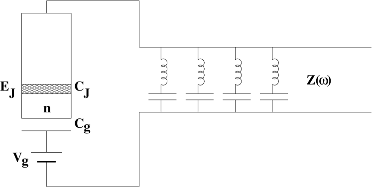
Figure 9: The qubit’s environment modeled by a transmission line.

Consider a transmission line, or $LC$-line, shown in Fig. 9. It amounts to an impedance $Z(\omega)$

$$Z^{-1}(\omega)=\sum_{a}\left(-i\omega L_{a}-{1\over i\omega C_{a}}+0\right)^{-1}=\sum_{a}{i\omega\over L_{a}(\omega^{2}-\omega^{2}_{a}+i0\mathop{\rm sign}\omega)}\ ,$$ (62)

with $\omega_{a}\equiv 1/\sqrt{L_{a}C_{a}}$ (index $a$ counts the $LC$ elements of the transmission line). The infinitesimal resistance in each $LC$-element serves to regularize the model. One way to derive the Hamiltonian is to start by introducing the degrees of freedom (the phase drops at circuit elements), writing the Lagrangian of the system (a combination of the charging and Josephson energies), and then performing the Legendre transformation. For convenience instead of the phase variables $\theta_{k}$ ($k$ being any index) we use the dimensionful flux variables $\phi_{k}=\Phi_{0}\theta_{k}/2\pi$ (defined as time integrals of respective voltage drops; here $\Phi_{0}=h/2e$), to which we still refer as ‘phases’. As independent variables one can use the phase on the Josephson junction $\phi_{\rm J}$, the phase between the terminals of the impedance $\phi$ and the phases on the capacitors of the $LC$ elements of the transmission line $\phi_{a}$. Then the phases on the inductances of the $LC$ elements are given by $\phi-\phi_{a}$, while the phase on the gate capacitor is given by the Kirchhof rule $\phi_{\rm g}=-(\phi_{\rm J}+\phi+\int V_{\rm g}dt^{\prime})$. The Lagrangian of the system reads

$$L=\frac{C_{\rm J}\,\dot{\phi}_{\rm J}^{2}}{2}+\frac{C_{\rm g}\,(\dot{\phi}_{\rm J}+\dot{\phi}+V_{\rm g})^{2}}{2}+E_{\rm J}\cos\left(2\pi\frac{\phi_{\rm J}}{\Phi_{0}}\right)+L_{Z}(\phi)\ ,$$ (63)

where

$$L_{Z}(\phi)\equiv\sum_{a}\left[\frac{C_{a}\dot{\phi}_{a}^{2}}{2}-\frac{(\phi_{a}-\phi)^{2}}{2L_{a}}\right]\ .$$ (64)

From here it is straightforward to derive the Hamiltonian of the system,

$$H=\frac{(2en-q)^{2}}{2C_{\rm J}}-E_{\rm J}\cos\theta+\frac{(q-C_{\rm g}V_{\rm g})^{2}}{2C_{\rm g}}+H_{Z}(\phi)\ ,$$ (65)

where

$$H_{Z}(\phi)\equiv\sum_{a}\left[\frac{q_{a}^{2}}{2C_{a}}+\frac{(\phi_{a}-\phi)^{2}}{2L_{a}}\right]\ .$$ (66)

Here $(n,\theta)$, $(q,\phi)$, $(q_{a},\phi_{a})$ are the pairs of conjugate variables, and $q=-C_{\rm g}\dot{\phi}_{g}$ is the charge on the gate capacitor. We assumed that the charge of the island $2en$ is completely located on the plates of the capacitors $C_{\rm J}$ and $C_{\rm g}$, and neglected the so-called offset charge induced by parasitic voltages due, e.g., to extra charges in the substrate. Introducing the new charge $\tilde{q}\equiv q-C_{\rm t}V_{\rm g}$ we obtain

$$H=\frac{(2en-C_{\rm t}V_{\rm g})^{2}}{2C_{\rm J}}-E_{\rm J}\cos\theta-\frac{2e}{C_{\rm J}}n\tilde{q}+C_{\rm t}\dot{V}_{\rm g}\phi+\frac{\tilde{q}^{2}}{2C_{\rm t}}+H_{Z}(\phi)\,,$$ (67)

thus recovering Eq. (7).

Indeed, the degrees of freedom $q_{a},\phi_{a}$ and $q,\phi$ play the part of the oscillator bath, its Hamiltonian being given by the last two terms in Eq. (67) (its eigenmodes are not given explicitly). Further, $\tilde{q}/C_{\rm t}=\delta V$ corresponds to the voltage fluctuations, and the first term in Eq. (67) coincides with the sum of the first and the last terms in Eq. (7). Notice that the last two terms in Eq. (67) describe a parallel connection of the impedance and an effective capacitance $C_{\rm t}$. Accordingly – one can check this also by an explicit calculation – the produced noise is given by Eq. (6), i.e., the bath ‘corresponds’ to the impedance $Z_{\rm t}$ rather than $Z$.

In this model one can also observe the result of an abrupt change of the gate voltage. It is most easily seen from Eqs. (65, 66) that the gate voltage is coupled to the qubit’s degree of freedom $n$ only via the damped mode $(q,\phi)$. As a result, for a pure resistor $Z(\omega)=R$ changes of $V_{\rm g}$ influence the qubit only after a delay time, of order $RC_{\rm t}$. In the form (67) the term proportional to the time derivative of $V_{\rm g}$ is responsible for this delay.

References

• Bloch (1946) Bloch, F.: 1946, ‘Nuclear induction’. Phys. Rev. 70, 460.
• Bloch (1957) Bloch, F.: 1957, ‘Generalized theory of relaxation’. Phys. Rev. 105, 1206.
• Caldeira and Leggett (1983) Caldeira, A. O. and A. J. Leggett: 1983, ‘Quantum tunnelling in a dissipative system’. Ann. Phys. (NY) 149, 374.
• Chiorescu et al. (2003) Chiorescu, I., Y. Nakamura, C. J. P. M. Harmans, and J. E. Mooij: 2003, ‘Coherent Quantum Dynamics of a Superconducting Flux Qubit’. Science 299, 1869.
• Cottet et al. (2001) Cottet, A., A. Steinbach, P. Joyez, D. Vion, H. Pothier, and M. E. Huber: 2001, ‘Superconducting Electrometer for Measuring the Single Cooper Pair Box’. In: D. V. Averin, B. Ruggiero, and P. Silvestrini (eds.): Macroscopic Quantum Coherence and Quantum Computing. New York, p. 111, Kluwer/Plenum.
• DiVincenzo (1997) DiVincenzo, D.: 1997, ‘Topics in quantum computers’. In: L. Kouwenhoven, G. Schön, and L. Sohn (eds.): Mesoscopic Electron Transport, Vol. 345 of NATO ASI Series E: Applied Sciences. Dordrecht, p. 657, Kluwer.
• Fazio et al. (1999) Fazio, R., G. M. Palma, and J. Siewert: 1999, ‘Fidelity and leakage of Josephson qubits’. Phys. Rev. Lett. 83, 5385.
• Ingold and Nazarov (1992) Ingold, G.-L. and Y. V. Nazarov: 1992, ‘Charge tunneling rates in ultrasmall junctions’. In: H. Grabert and M. H. Devoret (eds.): Single charge tunneling. N.Y., Plenum Press.
• Leggett et al. (1987) Leggett, A. J., S. Chakravarty, A. T. Dorsey, M. P. A. Fisher, A. Garg, and W. Zwerger: 1987, ‘Dynamics of the dissipative two-state system’. Rev. Mod. Phys. 59, 1.
• Makhlin and Shnirman (2003) Makhlin, Yu. and A. Shnirman: 2003, ‘Dephasing of solid-state qubits at optimal points’. cond-mat/0308297.
• Misra and Sudarshan (1977) Misra, B. and E. Sudarshan: 1977, ‘The Zeno’s paradox in quantum theory’. J. Math. Phys. 18, 756.
• Nakamura et al. (1999) Nakamura, Y., Yu. A. Pashkin, and J. S. Tsai: 1999, ‘Coherent control of macroscopic quantum states in a single-Cooper-pair box’. Nature 398, 786.
• Nakamura et al. (2002) Nakamura, Y., Yu. A. Pashkin, T. Yamamoto, and J. S. Tsai: 2002, ‘Charge echo in a Cooper-pair box’. Phys. Rev. Lett. 88, 047901.
• Paladino et al. (2003) Paladino, E., F. Taddei, G. Giaquinta, and G. Falci: 2003, ‘Josephson nanocircuit in the presense of linear quantum noise’. In: Proceedings of LT23, to appear in Physica E. cond-mat/0301363.
• Redfield (1957) Redfield, A. G.: 1957, ‘On the Theory of Relaxation Processes’. IBM J. Res. Dev. 1, 19.
• Schoeller and Schön (1994) Schoeller, H. and G. Schön: 1994, ‘Mesoscopic quantum transport: resonant tunneling in the presence of strong Coulomb interaction’. Phys. Rev. B 50, 18436.
• Shnirman et al. (2002) Shnirman, A., Yu. Makhlin, and G. Schön: 2002, ‘Noise and Decoherence in Quantum Two-Level Systems’. Phys. Scr. T102, 147.
• Vion et al. (2002) Vion, D., A. Aassime, A. Cottet, P. Joyez, H. Pothier, C. Urbina, D. Esteve, and M. H. Devoret: 2002, ‘Manipulating the quantum state of an electrical circuit’. Science 296, 886.
• Wangsness and Bloch (1953) Wangsness, R. K. and F. Bloch: 1953, ‘The dynamical theory of nuclear induction’. Phys. Rev. 89, 728.
• Weiss (1999) Weiss, U.: 1999, Quantum dissipative systems. Singapore: World Scientific, 2nd edition.