Bethe-ansatz studies of energy level crossings
in the one-dimensional Hubbard model

Abstract

Motivated by Heilmann and Lieb’s work [8], we discuss energy level crossings for the one-dimensional Hubbard model through the Bethe ansatz, constructing explicitly the degenerate eigenstates at the crossing points. After showing the existence of solutions for the Lieb–Wu equations with one-down spin, we solve them numerically and construct Bethe ansatz eigenstates. We thus verify all the level crossings in the spectral flows observed by the numerical diagonalization method with one down-spin. For each of the solutions we obtain its energy spectral flow along the interaction parameter $U$. Then, we observe that some of the energy level crossings can not be explained in terms of $U$-independent symmetries. Dynamical symmetries of the Hubbard model are fundamental for identifying each of the spectral lines at the level crossing points. We show that the Bethe ansatz eigenstates which degenerate at the points have distinct sets of eigenvalues of the higher conserved operators. We also show a twofold permanent degeneracy in terms of the Bethe ansatz wavefunction.

1 Introduction

Degeneracies in the energy spectra of quantum systems have close relationships with their symmetries. Actually, von Neumann and Wigner showed that degeneracies are more likely to occur for the systems with one or more symmetries than those without symmetries [20, 13]. To be more precise, if one assumes that a quantum system is given by a real Hamiltonian matrix whose elements are expressed by independent parameters, in the case of no symmetry, two parameters happen to take some prescribed values in order to bring two of the eigenvalues into coincidence. Their theory reminds us of the “non-crossing rule” in quantum chemistry, which states that energy levels of orbitals of the same symmetry can never cross each other along a reaction parameter. However, von Neumann–Wigner’s theorem does not give a proof for the non-crossing rule. It is possible that degeneracies appear in the systems without symmetries. Such degeneracies are referred to as accidental degeneracies. In fact some examples of accidental degeneracies are numerically observed in molecules [21] or triangular quantum billiards [1].

The one-dimensional Hubbard model is one of the most significant models in condensed matter physics. The model also attracts a great interest of mathematical physicists due to its Bethe-ansatz solvability [10, 9]. Heilmann and Lieb numerically investigated energy spectral flows along the interaction parameter $U$ for the system on a periodic 6-site chain and found many level crossings which can not be accounted for by the known symmetries such as translation, $SO(4)$ and particle-hole symmetries [8, 2]. They concluded that, if one takes into account only $U$-independent symmetries, the level crossings are accidental degeneracies, that is, a counter example of the non-crossing rule. Recently, Yuzbashyan, Altshuler and Shastry have suggested that the origin of Heilmann–Lieb’s level crossings should be dynamical symmetries in the Hubbard model [28]. Here the dynamical symmetries are given by parameter-dependent operators, which are often called higher conserved operators in association with conserved quantities in classical integrable systems. The dynamical symmetries for the Hubbard model are constructed in [14, 15, 7, 22, 11]. Yuzbashyan, Altshuler and Shastry numerically showed that crossings in the spectral flows of the first three conserved operators never occur at the same value of $U$. The dynamical symmetries depend on the parameter $U$, and they are not considered as symmetries in the von Neumann–Wigner’s theorem. Heilmann–Lieb’s level crossings are still considered to be accidental degeneracies.

In the framework of the Bethe ansatz, we discuss in the paper energy level crossings for the one-dimensional Hubbard model. The Bethe ansatz method provides information on the eigenstates that can not be easily obtained in the direct diagonalization of the Hamiltonian matrix. We set up the following problems:

1. When two energy eigenvalues approach in numerical data as one parameter is varied, one may draw two alternative spectral flows, a level crossing or level repulsion [8]. To ensure that genuine energy level crossings have happened, we must investigate the change of each eigenstate along the parameter $U$.

2. Do the eigenstates have distinct dynamical symmetries at the level crossing points? In order to solve the problem we assign each of the eigenstates the eigenvalues of the higher conserved operators.

It is indeed not easy to investigate these problems. For the triangular quantum billiards with two parameters, Berry and Wilkinson investigated the behaviour of eigenstates along a circuit of the crossing point in the parameter space so that they could verify the existence of genuine energy level crossings [1]. For general quantum systems, it is hard in practice to construct quantum many-body eigenstates. The task is also not easy even for the systems that can be treated by the Bethe ansatz. In fact, it is nontrivial to obtain numerical solutions to the Bethe ansatz equations for a finite size system. For the sector of one down-spin, however, it is practically possible to solve the Bethe ansatz equations numerically.

In the present paper, we prove the existence of solutions to the Lieb–Wu equations and then numerically solve them. Here we generalize the method of Ref. [3]. By using the numerical solutions, we analyse the behaviour of each of the degenerate eigenstates along the parameter $U$. We thus find several genuine level crossings of energy spectral flows with the same $U$-independent symmetries. The merit of this method is that the numerical solutions for the Lieb–Wu equations provide not only the eigenvalues of the higher conserved operators but also the one-to-one correspondence between their spectral lines and eigenstates. As a consequence, we observe that all the common eigenspaces of the first three higher conserved operators are one-dimensional in the subspaces with the same $U$-independent symmetries. Furthermore, when there are $U$-independent degeneracies (permanent degeneracies) in the spectral flow, the one-to-one correspondence plays an essential role in assigning to each of the degenerate eigenstates its eigenvalues of the dynamical symmetries at the energy level crossing points. By using the explicit form of the Bethe ansatz wavefunctions [23], we can derive the permanent degeneracies. We remark that the existence of level crossings also gives a necessary condition for algebraic independence of the three higher conserved operators in the subspaces.

This paper is organized as follows: first, in Section 2, we summarize the known results for the Hubbard model and prepare for the following sections. We list the known symmetries of the Hubbard model in 2.1 and review the Bethe ansatz method in 2.2. In 2.3 we prove the existence of solutions for the Lieb–Wu equations with one down-spin following the approach developed in [3]. Next, in Section 3, we analyse degeneracies in the energy spectrum of the Hubbard model by using both direct diagonalization of the Hamiltonian matrix and the Bethe ansatz method. In 3.1 we describe twofold permanent degeneracies arising from a reflection symmetry of the lattice. In 3.2 and 3.3 we investigate energy level crossings for the systems with two or three up-spins and one down-spin on a periodic 6-site chain. We find some genuine energy level crossings and see that the degenerate eigenstates can be classified by the eigenvalues of the higher conserved operators. The final section is devoted to concluding remarks.

2 Symmetries and Bethe ansatz method

We introduce the Hubbard model on a one-dimensional periodic $L$-site chain. Let $c_{is}^{\dagger}$ and $c_{is},(i\in\mathbb{Z}/L\mathbb{Z},s\in\{\uparrow,\downarrow\})$ be the creation and annihilation operators of electrons satisfying $\{c_{is},c_{jt}\}=\{c_{is}^{\dagger},c_{jt}^{\dagger}\}=0$ and $\{c_{is},c_{jt}^{\dagger}\}=\delta_{ij}\delta_{st}$, and define the number operators by $n_{is}:=c_{is}^{\dagger}c_{is}$. We consider the Fock space of electrons with the vacuum state $|0\rangle$. The one-dimensional Hubbard model is described by the following Hamiltonian acting on the Fock space:

$$H=-\sum_{i=1}^{L}\sum_{s=\uparrow,\downarrow}(c_{is}^{\dagger}c_{i+1,s}+c_{i+1,s}^{\dagger}c_{is})+U\sum_{i=1}^{L}\Big{(}n_{i\uparrow}-\frac{1}{2}\Big{)}\Big{(}n_{i\downarrow}-\frac{1}{2}\Big{)},$$ (2.1)

where $U(\in\mathbb{R}_{>0})$ is the interaction parameter. We consider the system for $L$ even throughout the article.

2.1 $U$-independent and dynamical symmetries

In general, the symmetries of a quantum system are expressed by operators which commute with its Hamiltonian. They are classified into two families in the case of the Hubbard model; one is independent of $U$ and another depends on $U$. We list some of these symmetries. First we consider the $U$-independent symmetries [8]. Define

$$\sigma:=\prod_{i=1}^{\frac{L}{2}-1}\prod_{s=\uparrow,\downarrow}P^{(s)}_{i,L-i},\quad\tau:=\prod_{s=\uparrow,\downarrow}P^{(s)}_{12}P^{(s)}_{23}\cdots P^{(s)}_{L-1,L},$$ (2.2)

where $P^{(s)}_{ij}:=1-(c_{is}^{\dagger}-c_{js}^{\dagger})(c_{is}-c_{js}),(i\neq j)$ are permutation operators. The operators $\sigma$ and $\tau$ correspond to reflection and translation symmetries of the lattice, respectively. They satisfy $\sigma^{2}=\tau^{L}=1$. It is clear that they commute with the Hamiltonian (2.1). Another $U$-independent symmetry is the $SO(4)$ symmetry [25, 26]. Define

$$S_{z}:=\frac{1}{2}\sum_{i=1}^{L}(n_{i\uparrow}-n_{i\downarrow}),\quad S_{+}:=\sum_{i=1}^{L}c_{i\uparrow}^{\dagger}c_{i\downarrow},\quad S_{-}:=(S_{+})^{\dagger},$$

$$\eta_{z}:=\frac{1}{2}\sum_{i=1}^{L}(1-n_{i\uparrow}-n_{i\downarrow}),\quad\eta_{+}:=\sum_{i=1}^{L}(-)^{i}c_{i\downarrow}c_{i\uparrow},\quad\eta_{-}:=(\eta_{+})^{\dagger}.$$ (2.3)

Both sets of operators $\{S_{z},S_{\pm}\}$ and $\{\eta_{z},\eta_{\pm}\}$ give representations of the algebra $\mathfrak{su}(2)$ in the Fock space. They all commute with the Hamiltonian (2.1), which leads to the symmetry of type $\mathfrak{su}(2)\oplus\mathfrak{su}(2)\simeq\mathfrak{so}(4)$. Furthermore it is known that this $\mathfrak{so}(4)$ symmetry lifts to the $SO(4)$ group symmetry. For the later discussion, we define Casimir operators,

$$\mbox{\boldmath$S$}^{2}:=\frac{1}{2}\Big{(}S_{+}S_{-}+S_{-}S_{+}\Big{)}+S_{z}^{2},\quad\mbox{\boldmath$\eta$}^{2}:=\frac{1}{2}\Big{(}\eta_{+}\eta_{-}+\eta_{-}\eta_{+}\Big{)}+\eta_{z}^{2},$$

which commute with all the operators in (2.1).

Next we introduce the dynamical symmetries given by the $U$-dependent operators. These $U$-dependent operators themselves are also commutative and are called conserved operators in association with conserved quantities in classical integrable systems. In [15, 7], the first three conserved operators are explicitly given by

$$I_{1}= H,$$

$$I_{2}= -\sqrt{-1}\sum_{i=1}^{L}\sum_{s=\uparrow,\downarrow}(c_{is}^{\dagger}c_{i+2,s}\!-\!c_{i+2,s}^{\dagger}c_{is})$$

$$\!+\!\sqrt{-1}U\sum_{i=1}^{L}\sum_{s=\uparrow,\downarrow}(c_{is}^{\dagger}c_{i+1,s}\!-\!c_{i+1,s}^{\dagger}c_{is})(n_{i,-s}\!+\!n_{i+1,-s}\!-\!1),$$

$$I_{3}= -\sum_{i=1}^{L}\sum_{s=\uparrow,\downarrow}(c_{is}^{\dagger}c_{i+3,s}+c_{i+3,s}^{\dagger}c_{is})$$

$$+U\sum_{i=1}^{L}\!\sum_{s=\uparrow,\downarrow}\Big{(}(c_{is}^{\dagger}c_{i+2,s}+c_{i+2,s}^{\dagger}c_{is})\Big{(}n_{i,-s}+n_{i+1,-s}+n_{i+2,-s}-\frac{3}{2}\Big{)}$$

$$\hskip 85.35826pt+(c_{i+1,s}^{\dagger}c_{i+2,s}\!-\!c_{i+2,s}^{\dagger}c_{i+1,s})(c_{i,-s}^{\dagger}c_{i+1,-s}\!-\!c_{i+1,-s}^{\dagger}c_{i,-s})$$

$$\hskip 85.35826pt+\frac{1}{2}(c_{i,s}^{\dagger}c_{i+1,s}\!-\!c_{i+1,s}^{\dagger}c_{i,s})(c_{i,-s}^{\dagger}c_{i+1,-s}\!-\!c_{i+1,-s}^{\dagger}c_{i,-s})$$

$$\hskip 85.35826pt-\Big{(}n_{is}\!-\!\frac{1}{2}\Big{)}\Big{(}n_{i+1,-s}\!-\!\frac{1}{2}\Big{)}-\frac{1}{2}\Big{(}n_{is}\!-\!\frac{1}{2}\Big{)}\Big{(}n_{i,-s}\!-\!\frac{1}{2}\Big{)}\Big{)}$$

$$-U^{2}\sum_{i=1}^{L}\!\sum_{s=\uparrow,\downarrow}(c_{is}^{\dagger}c_{i+1,s}+c_{i+1,s}^{\dagger}c_{is})\Big{(}n_{i,-s}n_{i+1,-s}\!-\!\frac{1}{2}(n_{i,-s}\!+\!n_{i+1,-s})\!+\!\frac{1}{2}\Big{)}.$$

In order to obtain higher conserved operators systematically, the transfer matrix approach similar to that of the XXZ Heisenberg spin chain is developed [14, 15, 22, 11]. The $SO(4)$ symmetry of such higher conserved operators is also verified in the framework of the transfer matrix approach [16].

The operators $\{\tau,\mbox{\boldmath$S$}^{2},S_{z},\mbox{\boldmath$\eta$}^{2},\eta_{z},I_{n}\}$ give a commutative set of operators including the Hamiltonian. Hence they can be diagonalized simultaneously.

2.2 Bethe ansatz method

The Bethe ansatz method was applied to the Hubbard model in [10]. Here we give only the result. Let $N$ be the number of electrons and $M$ that of down-spins. We may assume $2M\leq N\leq L$ due to particle-hole and spin reversal symmetries in the system. Let $k=\{k_{i}|i=1,2,\ldots,N\},(\mathrm{Re}(k_{i})\in\mathbb{R}/2\pi\mathbb{R})$ denote a set of wavenumbers of electrons and $\lambda=\{\lambda_{\alpha}|\alpha=1,2,\ldots,M\}$ that of rapidities of down-spins. Given a set of spin configuration $s=\{s_{i}|i=1,2,\ldots,N\}$ with $N-M$ up-spins and $M$ down-spins, the Bethe state with $k$ and $\lambda$ has the following form:

$$|k,\lambda;s\rangle=\sum_{\{x_{i}\}}\psi_{k,\lambda}(x;s)c_{x_{1},s_{1}}^{\dagger}c_{x_{2},s_{2}}^{\dagger}\cdots c_{x_{N},s_{N}}^{\dagger}|0\rangle.$$ (2.4)

The coefficients $\psi_{k,\lambda}(x;s)$ in (2.4) are expressed  [23] as

$$\psi_{k,\lambda}(x;s)=\sum_{P\in\mathfrak{S}_{N}}\mathrm{sign}(PQ)\varphi_{k_{P},\lambda}(s_{Q})\exp\Big{(}\sqrt{-1}\sum_{i=1}^{N}k_{P(i)}x_{Q(i)}\Big{)},$$

$$\varphi_{k_{P},\lambda}(s_{Q})=\sum_{R\in\mathfrak{S}_{M}}\prod_{\alpha<\beta}\frac{\lambda_{R(\alpha)}\!-\!\lambda_{R(\beta)}\!-\!\sqrt{-1}U/2}{\lambda_{R(\alpha)}\!-\!\lambda_{R(\beta)}}\prod_{\gamma=1}^{M}F_{k_{P}}(\lambda_{R(\gamma)},y_{\gamma}),$$

$$F_{k_{P}}(\lambda_{\alpha},y)=\frac{1}{\lambda_{\alpha}\!-\!\sin k_{P(y)}\!+\!\sqrt{-1}U/4}\prod_{j=1}^{y-1}\frac{\lambda_{\alpha}\!-\!\sin k_{P(j)}\!-\!\sqrt{-1}U/4}{\lambda_{\alpha}\!-\!\sin k_{P(j)}\!+\!\sqrt{-1}U/4},$$

where we have denoted by $Q$ one of the shortest elements in the symmetric group $\mathfrak{S}_{N}$ on $\{1,2,\ldots,N\}$ such that $1\leq x_{Q(1)}\leq x_{Q(2)}\leq\cdots\leq x_{Q(N)}\leq L$, and by $y_{\gamma}$ the position of the $\gamma$th down-spin in $s_{Q}=\{s_{Q(1)},s_{Q(2)},\ldots,s_{Q(N)}\}$. The Bethe states (2.4) give eigenstates of the Hamiltonian (2.1) if $\{k_{i},\lambda_{\alpha}\}$ satisfy the following equations:

$$\mathrm{e}^{\sqrt{-1}k_{i}L}=\prod_{\beta=1}^{M}\frac{\lambda_{\beta}-\sin k_{i}-\sqrt{-1}U/4}{\lambda_{\beta}-\sin k_{i}+\sqrt{-1}U/4},$$

$$\prod_{i=1}^{N}\frac{\lambda_{\alpha}-\sin k_{i}-\sqrt{-1}U/4}{\lambda_{\alpha}-\sin k_{i}+\sqrt{-1}U/4}=\prod_{\beta(\neq\alpha)}\frac{\lambda_{\alpha}-\lambda_{\beta}-\sqrt{-1}U/2}{\lambda_{\alpha}-\lambda_{\beta}+\sqrt{-1}U/2},$$ (2.5)

which are coupled nonlinear equations called Lieb–Wu equations. The Lieb–Wu equations have not been solved analytically. But it predicts some important results on thermodynamic properties of the system through Takahashi’s string hypothesis [17, 18, 9, 19].

The Bethe states (2.4) are not only eigenstates of the Hamiltonian (2.1) but also those of the translation operator $\tau$ and the higher conserved operators $I_{2}$ and $I_{3}$. By using the solutions $\{k_{i},\lambda_{\alpha}\}$ of the Lieb–Wu equations (2.2), the eigenvalues of $\tau$ and $\{I_{n}\}$ are written as

$$\tau|k,\lambda;s\rangle=\mathrm{e}^{\sqrt{-1}\frac{2\pi}{L}P}|k,\lambda;s\rangle,\quad P=\frac{L}{2\pi}\Big{(}\sum_{i=1}^{N}k_{i}\Big{)}\,(\mathrm{mod}\,L),$$

$$I_{n}|k,\lambda;s\rangle=E_{n}|k,\lambda;s\rangle,\quad(n=1,2,3),$$

$$E_{1}=E=-2\sum_{i=1}^{N}\cos k_{i}+\frac{1}{4}U(L\!-\!2N),$$

$$E_{2}=-2\sum_{i=1}^{N}\big{(}\sin(2k_{i})+U\sin k_{i}\big{)},$$

$$E_{3}=-\sum_{i=1}^{N}\Big{(}2\cos(3k_{i})+3U\Big{(}\!\cos(2k_{i})-\frac{1}{2}\Big{)}+U^{2}\cos k_{i}\Big{)}-\frac{3}{4}UL.$$ (2.6)

The $P$ appearing in the eigenvalues of $\tau$ indicates the total momentum of the system. (There should be no confusion with the use of $P$ in the coefficients of the Bethe states where $P$ denotes an element in $\mathfrak{S}_{N}$.)

We immediately find

$$S_{z}|k,\lambda;s\rangle=\frac{1}{2}(N-2M)|k,\lambda;s\rangle,\quad\eta_{z}|k,\lambda;s\rangle=\frac{1}{2}(L-N)|k,\lambda;s\rangle.$$ (2.7)

It is shown in [6] that each Bethe state (2.4) with a regular solution for the Lieb–Wu equations (2.2) corresponds to the highest weight vector of a highest weight representation of $\mathfrak{so}(4)$, i.e., $S_{+}|k,\lambda;s\rangle=\eta_{+}|k,\lambda;s\rangle=0$. Then we find

$$\mbox{\boldmath$S$}^{2}|k,\lambda;s\rangle=S(S+1)|k,\lambda;s\rangle,\quad\mbox{\boldmath$\eta$}^{2}|k,\lambda;s\rangle=\eta(\eta+1)|k,\lambda;s\rangle,$$ (2.8)

with $S=(N-2M)/2$ and $\eta=(L-N)/2$. Hence, by applying the lowering operators $(S_{-})^{n},(0\leq n\leq N-2M)$ and $(\eta_{-})^{m},(0\leq m\leq L-N)$ to the Bethe states (2.4), we also have eigenstates of the Hubbard Hamiltonian (2.1),

$$|k,\lambda;s;n,m\rangle:=(S_{-})^{n}(\eta_{-})^{m}|k,\lambda;s\rangle,\quad$$ (2.9)

which have the same eigenvalues $\{E_{n}\}$ for the operators $\{I_{n}\}$ as those of $|k,\lambda;s\rangle$. The dimension of the representation with the highest weight vector $|k,\lambda;s\rangle$ is $(N-2M+1)(L-N+1)$. By using Takahashi’s string hypothesis for the Bethe states (2.4) together with the $\mathfrak{so}(4)$ symmetry, their combinatorial completeness is proved in [5].

2.3 Lieb–Wu equations with one down-spin

We try to find regular solutions of the Lieb–Wu equations (2.2) in the case when the system has only one down-spin following the discussion in [3]. In this case, the string hypothesis [17] predicts that two types of solutions exist: one is the solution with only real wavenumbers $\{k_{i}\}$ and another includes two complex wavenumbers. First we consider the real wavenumber solutions. For $M=1$, the Lieb–Wu equations (2.2) reduce to

$$\mathrm{e}^{\sqrt{-1}k_{i}L}=\frac{\lambda-\sin k_{i}-\sqrt{-1}U/4}{\lambda-\sin k_{i}+\sqrt{-1}U/4},\quad(i=1,2,\ldots,N),$$

$$\prod_{i=1}^{N}\frac{\lambda-\sin k_{i}-\sqrt{-1}U/4}{\lambda-\sin k_{i}+\sqrt{-1}U/4}=1.$$ (2.10)

These are equivalent to the following equations:

$$\sin k_{i}-\lambda=\frac{U}{4}\cot\Big{(}\frac{k_{i}L}{2}\Big{)},\quad\exp\Big{(}\sqrt{-1}\sum_{i=1}^{N}k_{i}L\Big{)}=1.$$ (2.11)

We consider the real solutions for the first equation

$$\sin q-\lambda=\frac{U}{4}\cot\Big{(}\frac{qL}{2}\Big{)}.$$ (2.12)

In the interval $0\leq q<2\pi$, its right hand side has $L$ branches

$$\frac{2\pi}{L}\Big{(}\ell-\frac{1}{2}\Big{)}<q<\frac{2\pi}{L}\Big{(}\ell+\frac{1}{2}\Big{)},\quad\ell\in\Big{\{}\frac{2j-1}{2}\Big{|}j=1,2,\ldots,L\Big{\}}.$$ (2.13)

If we seek a solution $q$ of (2.12) in one of the branches (2.13), the solution is unique under the condition $UL>8$ [3] and can be written as a function of $\lambda$, i.e., $q=q_{\ell}(\lambda)$. Given a distinct set $\{\ell_{i}|i=1,2,\ldots,N\}\subset\{\frac{2j-1}{2}|j=1,2,\ldots,L\}$ of the branches, the second equation in (2.12) is satisfied when $\frac{L}{2\pi}\sum_{i=1}^{N}q_{\ell_{i}}(\lambda)\in\mathbb{Z}$. The behaviour of the solution $q=q_{\ell}(\lambda)$ tells us that

$$\lim_{\lambda\to\pm\infty}\frac{L}{2\pi}\sum_{i=1}^{N}q_{\ell_{i}}(\lambda)=\sum_{i=1}^{N}\Big{(}\ell_{i}\pm\frac{1}{2}\Big{)}.$$ (2.14)

Hence there exist $N-1$ values of $\lambda$ which give the following integer values for $\frac{L}{2\pi}\sum_{i=1}^{N}q_{\ell_{i}}(\lambda)$:

$$m\in\Bigg{\{}\sum_{i=1}^{N}\Big{(}\ell_{i}-\frac{1}{2}\Big{)}+j\Bigg{|}j=1,2,\cdots,N-1\Bigg{\}}.$$

Note that such $\{\lambda\}$ and integers $\{m\}$ are in one-to-one correspondence due to $\frac{dq_{\ell}(\lambda)}{d\lambda}>0$. It is straightforward that $\{k_{i}=q_{\ell_{i}}(\lambda),\lambda\}$ characterized by the indices $\{\ell_{i},m\}$ give $\big{(}{L\atop N}\big{)}(N-1)$ solutions of the equations (2.11).

Next we consider the $k$-$\Lambda$-string solutions. We assume the forms of solutions as

$$k_{i}\in\mathbb{R}/2\pi\mathbb{R},\;(i=1,2,\ldots,N-2),\quad k_{N-1}=\zeta\!-\!\sqrt{-1}\xi,\quad k_{N}=\zeta\!+\!\sqrt{-1}\xi,$$

where $0\leq\zeta<2\pi$ and $\xi>0$. Note that $k_{N-1}$ and $k_{N}$ form a complex conjugate pair which is referred to as $k$-$\Lambda$-two-string. Then the first equations in (2.3) are rewritten as the following equations with real variables:

$$\sin k_{i}-\lambda=\frac{U}{4}\cot\Big{(}\frac{k_{i}L}{2}\Big{)},\quad(i=1,2,\ldots,N-2),$$ (2.15a)

$$\sin\zeta\cosh\xi-\lambda=\frac{U}{4}\frac{\sin(\zeta L)}{\cosh(\xi L)-\cos(\zeta L)},$$ (2.15b)

$$\cos\zeta\sinh\xi=-\frac{U}{4}\frac{\sinh(\xi L)}{\cosh(\xi L)-\cos(\zeta L)}.$$ (2.15c)

On the other hand, the second equation in (2.3) is equivalent to the following condition:

$$\sum_{i=1}^{N-2}k_{i}+2\zeta=\frac{2\pi}{L}m,\quad(m\in\{0,1,\ldots,NL-1\}).$$ (2.16)

In the same way as the previous case, if we consider a solution of each equation (2.15a) in one of the branches (2.13), it can be written as a function of $\lambda$. Given a distinct set $\{\ell_{i}|i=1,2,\ldots,N-2\}$ of indices specifying the branches (2.13), we express the solutions of (2.15a) as $k_{i}=q_{\ell_{i}}(\lambda),(i=1,2,\ldots,N-2)$. Then, from the relation (2.16), the $\zeta$ is also written as a function of $\lambda$,

$$\zeta=\zeta(\lambda):=\frac{\pi}{L}m-\frac{1}{2}\sum_{i=1}^{N-2}q_{\ell_{i}}(\lambda),$$ (2.17)

for fixed $\{\ell_{i}\}$ and $m$. For an illustration, we consider (2.15b) and (2.15c) in the case $N=2$. Since $\zeta$ does not depend on $\lambda$ in the case, the equations (2.15b) and (2.15c) decouple into

$$\lambda=\sin\Big{(}\frac{\pi}{L}m\Big{)}\cosh\xi,\quad\sinh\xi=-\frac{U}{4\cos(\frac{\pi}{L}m)}f^{(2)}(\xi),$$ (2.18)

where

$$f^{(2)}(\xi):=\frac{\sinh(\xi L)}{\cosh(\xi L)-(-1)^{m}}=\begin{cases}\tanh(\xi L/2)&\text{for }m\text{ odd},\\ \coth(\xi L/2)&\text{for }m\text{ even}.\\ \end{cases}$$

One finds from graphical discussion [3] that, if the condition $UL>8$ is satisfied, the second equation determines an unique $\xi(>0)$ for $\frac{\pi}{2}<\frac{\pi}{L}m<\frac{3\pi}{2}$. We denote it as $\xi_{m}^{(2)},(m\in\{\frac{L}{2}+j|j=1,2,\cdots,L-1\})$. The first equation in (2.18) immediately gives $\lambda$ with the $\xi_{m}^{(2)}$. Let us consider the case $N>2$. By inserting (2.17) into (2.15c), we have

$$\sinh\xi=-\frac{U}{4\cos(\zeta(\lambda))}f(\xi),\quad f(\xi):=\frac{\sinh(\xi L)}{\cosh(\xi L)-(-)^{m}\cos\big{(}\frac{L}{2}\sum_{i}q_{\ell_{i}}(\lambda)\big{)}}.$$ (2.19)

Since $f(\xi)>0$ for $\xi>0$ in the similar to the case $N=2$, this determines an unique $\xi$ as a function of $\lambda$ if and only if $\frac{\pi}{2}<\zeta(\lambda)=\frac{\pi}{L}m-\frac{1}{2}\sum_{i}q_{\ell_{i}}(\lambda)<\frac{3\pi}{2}$. By using (2.14), it is sufficient to have an unique solution for (2.19) that the integer $m$ satisfies

$$\sum_{i=1}^{N-2}\Big{(}\ell_{i}+\frac{1}{2}\Big{)}+\frac{L}{2}<m<\sum_{i=1}^{N-2}\Big{(}\ell_{i}-\frac{1}{2}\Big{)}+\frac{3L}{2},$$

that is,

$$m\in\Bigg{\{}\sum_{i=1}^{N-2}\Big{(}\ell_{i}+\frac{1}{2}\Big{)}+\frac{L}{2}+j\Bigg{|}j=1,2,\ldots,L-N+1\Bigg{\}}.$$ (2.20)

Note that $\lim_{\lambda\to\pm\infty}\xi(\lambda)=\xi_{m-\sum_{i}(\ell_{i}\pm\frac{1}{2})}^{(2)}$ which is well-defined for the above $m$. We expect that, for the $L-N+1$ values of $m$ allowed in (2.20), the equation (2.15b) with $\xi(\lambda)$ and $\zeta(\lambda)$

$$\lambda =\sin\big{(}{\textstyle\frac{\pi}{L}m\!-\!\frac{1}{2}\sum_{i}q_{\ell_{i}}(\lambda)}\big{)}\cosh\big{(}\xi(\lambda)\big{)}-\frac{U}{4}\frac{\sin(\frac{L}{2}\sum_{i}q_{\ell_{i}}(\lambda))}{\cos\big{(}\frac{L}{2}\sum_{i}q_{\ell_{i}}(\lambda)\big{)}-(-)^{m}\cosh\big{(}\xi(\lambda)L\big{)}}$$

$$=:g\big{(}q_{\ell_{i}}(\lambda),\xi(\lambda)\big{)},$$ (2.21)

determines $\lambda$. In fact, since $q_{\ell_{i}}(\lambda)$ and $\xi(\lambda)$ are continuous functions with respect to $\lambda$ and

$$\lim_{\lambda\to\pm\infty}g\big{(}q_{\ell_{i}}(\lambda),\xi(\lambda)\big{)}=g\Big{(}{\textstyle\frac{2\pi}{L}(\ell_{i}\pm\frac{1}{2}),\xi_{m-\sum_{i}(\ell_{i}\pm\frac{1}{2})}^{(2)}}\Big{)},$$

$g$ is a continuous and finite function with respect to $\lambda$. Hence there exists a solution $\lambda$ in (2.3). As a consequence we have $({L\atop N-2})(L-N+1)$ solutions corresponding to the indices $\{\ell_{i},m\}$.

Let us see the relation between the string hypothesis [17] and our results. Let $\{\ell_{i}\}$ reduce modulo $L$ into the interval $[-\frac{L}{2},\frac{L}{2})$ and express them as $\{I^{(i)}\}$. Putting $J=m-\sum_{i=1}^{N}\ell_{i}$ for the real wavenumber solutions and $J^{\prime}=L-m+\sum_{i=1}^{N-2}\ell_{i}$ for the $k$-$\Lambda$-two-string solution, we have

$$I^{(i)}\in\mathbb{Z}+\frac{1}{2},\quad-\frac{L}{2}<I^{(i)}\leq\frac{L}{2},$$

$$J\in\mathbb{Z}+\frac{N}{2},\quad|J|\leq\frac{1}{2}(N-2),\quad J^{\prime}\in\mathbb{Z}+\frac{N}{2},\quad|J^{\prime}|\leq\frac{1}{2}(L-N).$$ (2.22)

One sees that the indices $\{I^{(i)};J;J^{\prime}\}$ characterizing the regular solutions of the Lieb–Wu equations with $M=1$ are nothing but those appearing in the string hypothesis [17]. Thus we have shown for the Lieb–Wu equations (2.2) with $M=1$ that there exist the same number of solutions as those predicted by the string hypothesis. In the next section, we numerically calculate the solutions $\{k_{i},\lambda|i=1,2,\ldots,N\}$ and $\{k_{i},\zeta,\xi,\lambda|i=1,2,\ldots,N-2\}$ for $L=6$.

3 Energy level crossings

Let us review von Neumann–Wigner’s discussion on the spectra of quantum systems. We assume that a Hamiltonian is described by a finite-dimensional real symmetric matrix whose elements are regarded as random independent parameters. If the system has no symmetry, we call its spectra a “pure sequence”. If there exist some symmetries in the system, its spectra is given by a superposition of pure sequences, which we call a “mixed sequence”. Von Neumann–Wigner’s theorem reads as follows: one must adjust two parameters to bring two of the eigenvalues belonging to a pure sequence into coincidence while in a mixed sequence one obtain a degeneracy by varying only one parameter [20, 13]. Hence the degeneracies in pure sequences are very unlikely to be found if we choose the values of parameters in an arbitrary manner. Such degeneracies in pure sequences are referred to as accidental degeneracies.

Applying the above discussion, we study the Hubbard model. In varying the parameter $U$, the Hamiltonian (2.1) gives a flow in the above space of parameters. As we have mentioned in the previous section, the system has several symmetries. Since the operators $\{\tau,\mbox{\boldmath$S$}^{2},S_{z},\mbox{\boldmath$\eta$}^{2},\eta_{z}\}$ are mutually commutative, they can be simultaneously diagonalized by an orthogonal transformation. Through the same orthogonal transformation, the Hamiltonian matrix breaks up into diagonal blocks corresponding to the common eigenspaces of $\{\tau,\mbox{\boldmath$S$}^{2},S_{z},\mbox{\boldmath$\eta$}^{2},\eta_{z}\}$. Notice that the common eigenspaces are characterized by the set of quantum numbers $\{N,M,P,S,\eta\}$. Energy eigenvalues from the blocks with different quantum numbers may degenerate due to translation and $SO(4)$ symmetries. But all the blocks do not give a pure sequence; for example, the blocks with $L=N=2M$ have particle-hole and spin reversal symmetries. However, after considering all the known $U$-independent symmetries, the spectra also have many degeneracies at special values of $U$, i.e., level crossings in the spectral flows along the parameter $U$ [8]. Thus the flow determined by the Hamiltonian (2.1) runs through several special values of parameters that give accidental degeneracies.

Let us discuss how to numerically determine level crossings, in particular, for the case of accidental degeneracies. One notices that the numerical diagonalization of the Hamiltonian is not enough to find crossings of energy spectral flows since apparent crossings may be just close approaches of two eigenvalues [8]. To verify the existence of genuine level crossings, we must investigate the behaviour of spectral flows for each eigenstate. The Bethe ansatz method is a very effective tool to establish this. Here we restrict our investigation to the systems with one down-spin where we have shown the existence of solutions for the Lieb–Wu equations (2.2) in Subsection 2.3. We have seen in Subsection 2.1 that the Hubbard model has the dynamical symmetries in addition to the $U$-independent symmetries. The recent paper [28] pointed out that the degenerate eigenstates at the accidental degeneracies observed in [8] can be classified by the eigenvalues of the higher conserved operators. We verify their assertion at the level of eigenstates in the sector of one down-spin. Here we note that the degeneracies discussed in [8, 2, 28] are in the half-filled Hubbard model with zero magnetization, that is, in the sector of three down-spins. The strategy in the present paper is given by the following:

• We give a matrix representation of the Hamiltonian in a certain common eigenspace of the operators $\{\tau,\mbox{\boldmath$S$}^{2},S_{z},\mbox{\boldmath$\eta$}^{2},\eta_{z}\}$, which is referred to as desymmetrization of the corresponding symmetries. We numerically give its eigenvalues from the direct diagonalization [8, 28] for several values of $U$.

• We give the numerical solutions of the Lieb–Wu equations (2.2) in several values of $U$. From the correspondence between energy spectral flows and the Bethe states, we verify whether or not genuine energy level crossings exist.

• We also diagonalize other conserved operators $\{I_{2},I_{3}\}$ and see the correspondence between their spectral flows and the Bethe states. We analyse the structure of their degeneracies.

We discuss only the systems containing two or three up-spins and one down-spin, which do not have particle-hole and spin reversal symmetries. In spite of such restriction, we have some non-trivial results on degeneracies.

3.1 Twofold permanent degeneracies

The translation and the $SO(4)$ symmetries produce $U$-independent degeneracies in energy spectral flows. We call $U$-independent degeneracies permanent degeneracies. Furthermore, after the desymmetrization of these $U$-independent symmetries, we often observe another twofold permanent degeneracies associated with a reflection symmetry of the lattice [28]. In fact, we can explain them in terms of the Bethe ansatz wavefunction. Here we note that, due to the relation $\tau\sigma=\sigma\tau^{-1}$, the reflection operator $\sigma$ acts only on the eigenspaces of $\tau$ with the eigenvalue $1$ or $-1$, that is, the subspaces of the Fock space with the total momentum $P=0$ or $\frac{L}{2}$.

Let us investigate the twofold permanent degeneracies due to the reflection operator $\sigma$ in the framework of the Bethe ansatz method. Even in the subspaces with $P=0$ or $\frac{L}{2}$, the Bethe states do not always diagonalize the operator $\sigma$. Indeed it is easy to verify that, if we apply the operator $\sigma$ to one of the eigenvectors $|k,\lambda;s;m,n\rangle$, then its total momentum and eigenvalues of $\{I_{2n}\}$ are negated and those of $\{\mbox{\boldmath$S$}^{2},S_{z},\mbox{\boldmath$\eta$}^{2},\eta_{z},I_{2n-1}\}$ do not change since

$$\sigma\tau=\tau^{-1}\sigma,\quad\sigma I_{2n}+I_{2n}\sigma=0,\quad\sigma I_{2n-1}=I_{2n-1}\sigma,\quad[\sigma,S_{z,\pm}]=[\sigma,\eta_{z,\pm}]=0.$$ (3.1)

These facts are verified more directly from the following relation:

$$\sigma|k,\lambda;s;n,m\rangle=(-)^{M}|-k,-\lambda;s;n,m\rangle,$$ (3.2)

where $-k=\{-k_{i}|i=1,2,\ldots,N\}$ and $-\lambda=\{-\lambda_{\alpha}|\alpha=1,2,\ldots,M\}$. Note that, if $\{k_{i},\lambda_{\alpha}\}$ is a solution for the Lieb–Wu equations (2.2), then so is $\{-k_{i},-\lambda_{\alpha}\}$. The relation (3.2) means that, if the set $\{k_{i};\lambda_{\alpha}\}$ does not coincide with $\{-k_{i};-\lambda_{\alpha}\}$ as a set, we have a twofold permanent degeneracy in energy spectral flows. On the other hand, if $\{k_{i};\lambda_{\alpha}\}=\{-k_{i};-\lambda_{\alpha}\}$ as a set, then the eigenstates $|k,\lambda;s;m,n\rangle$ have the eigenvalue $E_{2}=0$ for the second conserved operator $I_{2}$, which follows from the formulas in (2.2). It should be noted that, to see the existence of such twofold permanent degeneracies, we must solve the Lieb–Wu equations (2.2).

3.2 Spectral flows: $L=6,N=3,M=1$

We now study the system with two up-spins and one down-spin on benzene ($L=6,N=3,M=1$). Note that $S_{z}=\frac{1}{2}$ and $\eta_{z}=\frac{3}{2}$ in this case. We consider the subspace characterized by the set of quantum numbers $\{P=2,S=\frac{1}{2},\eta=\frac{3}{2}\}$. There is no more $U$-independent symmetry in the subspace, and we shall actually find one of the simplest nontrivial energy level crossings there. We have a matrix representation of the Hamiltonian of $11$ dimension. We put $u:=U/(U+4)$ and numerically diagonalize the Hamiltonian matrix for several values of $u$. Figure 1 shows the energy spectral flows for $0<u<1$. Here the vertical line in the figure indicates the energy $E$ divided by $U+4$. We confirm from the numerical data that there is no permanent degeneracy. We observe a close approach of two energy levels in $0.5<u<0.6$, which seems to be an energy level crossing.

Our first purpose is to show that a genuine energy level crossing has been found in Figure 1. In the case of triangular quantum billiards [1], topological properties of their eigenstates were studied to verify the existence of energy level crossings. Here we employ the Bethe ansatz method to verify energy level crossings in the level of eigenstates. It is clear that, since $S=S_{z}=\frac{1}{2}$ and $\eta=\eta_{z}=\frac{3}{2}$, all the eigenstates in the subspace are the Bethe states characterized by the indices $\{I^{(i)};J;J^{\prime}\}$ satisfying (2.3). By using the procedure in Subsection 2.3, we numerically give real wavenumber solutions with $P=(\sum_{i=1}^{3}I^{(i)}+J)\,(\mathrm{mod}\,6)=2\,(\mathrm{mod}\,6)$ and $k$-$\Lambda$-two-string solutions with $P=(I^{(1)}-J^{\prime})\,(\mathrm{mod}\,6)=2\,(\mathrm{mod}\,6)$ to calculate the corresponding energy eigenvalues. The correspondence between energy eigenvalues and the Bethe states at $u=0.3$ and $0.8$ is displayed on Table 1. Here we deal with the Lieb–Wu equations only in the case when the condition $UL>8$ is satisfied. One sees that the results for $u\to 1,(U\to\infty)$ read as

$$\lim_{U\to\infty}\frac{E}{U+4}=\begin{cases}0&\text{for real wavenumber solutions,}\\ 1&\text{for $k$-$\Lambda$-two-string solutions,}\\ \end{cases}$$

which agrees with those conjectured by the string hypothesis. We remark that the energy eigenvalues obtained by the solutions of the Lieb–Wu equations coincide with those obtained by the direct diagonalization of the Hamiltonian matrix within an error of $O(10^{-15})$. Thus, by combining the results in Figure 1 with those on Table 1, we obtain the behaviour of energy spectral flows for each eigenstate. We conclude that, in $0.5<u<0.6$, there exists an energy level crossing between two Bethe states indexed by $\{-\frac{5}{2},\frac{3}{2},\frac{5}{2};\frac{1}{2};\}$ and $\{\frac{1}{2};;-\frac{3}{2}\}$.

Next we show that, if we take into account dynamical symmetries, each one-dimensional component of the degenerate eigenstates at the energy level crossing point can be distinguished from the other degenerate eigenstates. In the similar way to the energy eigenvalues, the eigenvalues of the second conserved operator $I_{2}$ are obtained by both their direct diagonalization and the solutions of the Lieb–Wu equations, which are displayed in Figure 2 and Table 2 (the vertical line in the figure also indicates the eigenvalue $E_{2}$ divided by $U+4$). Note that there is no permanent degeneracy. We observe that the spectral flows indexed by $\{-\frac{5}{2},\frac{3}{2},\frac{5}{2};\frac{1}{2};\}$ and $\{\frac{1}{2};;-\frac{3}{2}\}$ in Figure 2 never have crossings. Hence the Bethe states indexed by $\{-\frac{5}{2},\frac{3}{2},\frac{5}{2};\frac{1}{2};\}$ and $\{\frac{1}{2};;-\frac{3}{2}\}$ belong to different eigenspaces of $I_{2}$, that is, the two Bethe states have a different dynamical symmetry. Thus all the common eigenspaces of the operators $\{H,I_{2}\}$ with the set of quantum numbers $\{P=2,S=S_{z}=\frac{1}{2},\eta=\eta_{z}=\frac{3}{2}\}$ are one-dimensional.

Figure 1: Spectral flows $E$ from direct diagonalization for $L=6,N=3,M=1$, $P=2,S=\frac{1}{2}$ and $\eta=\frac{3}{2}$.

	$E/(U+4)$
$\{I^{(i)};J;J^{\prime}\}$	$u=0.3$	$u=0.8$	$u=1.0$
$\{\frac{5}{2};;\frac{1}{2}\}$	$\;\;1.005067890492477$	$\;\;0.9123001584634441$	$\;\;1$
$\{-\frac{5}{2};;\frac{3}{2}\}$	$\;\;0.6786192438740763$	$\;\;0.8733443175466562$	$\;\;1$
$\{\frac{3}{2};;-\frac{1}{2}\}$	$\;\;0.5258327541688925$	$\;\;0.8031341881381975$	$\;\;1$
$\{-\frac{5}{2},\frac{3}{2},\frac{5}{2};\frac{1}{2};\}$	$\;\;0.4763789806072449$	$\;\;0.1794157938506165$	$\;\;0$
$\{\frac{1}{2};;-\frac{3}{2}\}$	$\;\;0.144465968291432$	$\;\;0.7105015978852069$	$\;\;1$
$\{-\frac{3}{2},\frac{3}{2},\frac{5}{2};-\frac{1}{2};\}$	$-0.03872530249182613$	$\;\;0.06204279614552415$	$\;\;0$
$\{-\frac{5}{2},-\frac{3}{2},\frac{1}{2};-\frac{1}{2};\}$	$-0.05950271399595123$	$\;\;0.01208774945632921$	$\;\;0$
$\{-\frac{3}{2},\frac{1}{2},\frac{5}{2};\frac{1}{2};\}$	$-0.1292149141454342$	$-0.008632714879121293$	$\;\;0$
$\{-\frac{5}{2},-\frac{3}{2},-\frac{1}{2};\frac{1}{2};\}$	$-0.1472919189221319$	$-0.03595459977202529$	$\;\;0$
$\{-\frac{1}{2},\frac{1}{2},\frac{5}{2};-\frac{1}{2};\}$	$-0.447930438860179$	$-0.0995848490575883$	$\;\;0$
$\{-\frac{1}{2},\frac{1}{2},\frac{3}{2};\frac{1}{2};\}$	$-0.6326995490186007$	$-0.1586544377772396$	$\;\;0$

Table 1: $E$ obtained by the Bethe ansatz method.

Figure 2: Spectral flows $E_{2}$ from direct diagonalization for $L=6,N=3,M=1$, $P=2,S=\frac{1}{2}$ and $\eta=\frac{3}{2}$.

	$E_{2}/(U+4)$
$\{I^{(i)};J;J^{\prime}\}$	$u=0.3$	$u=0.8$
$\{-\frac{5}{2},-\frac{3}{2},-\frac{1}{2};\frac{1}{2};\}$	$\;\;1.373365167833861$	$\;\;3.179687928057096$
$\{-\frac{5}{2},\frac{3}{2},\frac{1}{2};-\frac{1}{2};\}$	$\;\;0.4945223061494427$	$\;\;1.493828870394599$
$\{-\frac{5}{2};;\frac{3}{2}\}$	$\;\;0.3397777976721251$	$\;\;1.117455777165958$
$\{-\frac{3}{2},\frac{1}{2},\frac{5}{2};\frac{1}{2};\}$	$\;\;0.2072047205613698$	$\;\;0.01309975997192909$
$\{-\frac{1}{2},\frac{1}{2},\frac{5}{2};-\frac{1}{2};\}$	$\;\;0.01863957159436896$	$-0.4919569001978466$
$\{\frac{5}{2};;\frac{1}{2}\}$	$-0.02590156370174922$	$-0.6254191358761778$
$\{-\frac{3}{2},\frac{3}{2},\frac{5}{2};-\frac{1}{2};\}$	$-0.1828197100832381$	$-0.9968145682615939$
$\{\frac{1}{2};;-\frac{3}{2}\}$	$-0.3289755229197938$	$-0.3593561303568662$
$\{-\frac{5}{2},\frac{3}{2},\frac{5}{2};\frac{1}{2};\}$	$-0.5374256073807519$	$-1.059175160002318$
$\{\frac{3}{2};;-\frac{1}{2}\}$	$-0.9702596151665846$	$-1.610420144313048$
$\{-\frac{1}{2},\frac{1}{2},\frac{3}{2};\frac{1}{2};\}$	$-1.210851678154266$	$-2.13317348301527$

Table 2: $E_{2}$ obtained by the Bethe ansatz method.

The fact that the common eigenspaces of $\{H,I_{2}\}$ are one-dimensional becomes clearer by investigating the spectral flows of the transfer matrix, i.e., the spectral flow sets of conserved operators. Figure 3 shows that, if we consider the eigenvalue sets $\{E,E_{2}\}$ for two of the eigenvectors along the parameter $U$, there is no crossing while their projection onto the $U$-$E$ plane has a crossing. One notices that the Bethe ansatz method plays an essential role in getting such picture. It seems to be rare that the eigenvalues of the transfer matrix simultaneously degenerate. We comment that the XXZ Heisenberg spin chain at root of unity has such degeneracies in the transfer matrix [4], where one sees symmetries defined only at the special values of parameters.

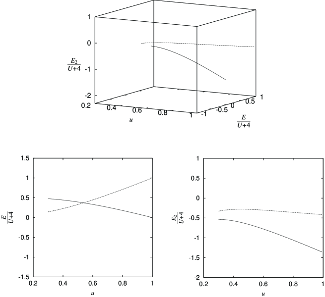
Figure 3: Spectral flow sets $(E,E_{2})$ characterized by $\{-\frac{5}{2},\frac{3}{2},\frac{5}{2};\frac{1}{2};\}$ and $\{\frac{1}{2};;-\frac{3}{2}\}$ for the system with $L=6,N=3,M=1$, $P=2,S=\frac{1}{2}$ and $\eta=\frac{3}{2}$, and their projections onto the $U$-$E$ and $U$-$E_{2}$ planes.

3.3 Spectral flows: $L=6,N=4,M=1$

We give an example where the eigenvalues $E$ and $E_{2}$ degenerate at the same value of $U$. We consider the system with three up-spins and one down-spin on benzene ($L=6,N=4,M=1$). In this case, we have $S_{z}=\eta_{z}=1$. We investigate the degeneracies of energy spectral flows in the subspace characterized by the set of quantum numbers $\{P=0,S=\eta=1\}$; hence we can expect all the eigenstates therein to be the Bethe states. The subspace is 14 dimensions. Figure 4 shows the energy spectral flows obtained by the numerical diagonalization of the Hamiltonian matrix for $0<u<1$. Also listed on Table 3 are the energy eigenvalues given by numerical solutions for the Lieb–Wu equations at $u=0.4$ and $0.8$; we show the numerical solutions in Appendix A. We observe as $u\to 1,(U\to\infty)$ that

$$\lim_{U\to\infty}\frac{E}{U+4}=\begin{cases}-\frac{1}{2}&\text{for real wavenumber solutions,}\\ \frac{1}{2}&\text{for $k$-$\Lambda$-two-string solutions,}\\ \end{cases}$$

which are also derived from the string hypothesis [17]. Here we note that the results from the two different methods above coincide within an error of $O(10^{-15})$, which give an evidence for the validity of the Bethe ansatz method. From Figure 4 and Table 3, we see the correspondence between the energy spectral flows and the indices $\{I^{(i)};J;J^{\prime}\}$ (2.3) characterizing the Bethe states. The correspondence shows that, if $\{I^{(i)};J;J^{\prime}\}\neq\{-I^{(i)};-J;-J^{\prime}\}$, i.e., $\{k_{i};\lambda\}\neq\{-k_{i};-\lambda\}$ as a set, two Bethe states characterized by these indices are in a permanent degeneracy. In fact, among the 14 Bethe states, 8 of them are in the twofold permanent degeneracies associated with the reflection symmetry. We find that the Bethe states indexed by $\{-\frac{5}{2},-\frac{3}{2},\frac{3}{2},\frac{5}{2};0;\}$ and $\{-\frac{1}{2},\frac{1}{2};;0\}$ has an energy level crossing at $u=0.5,(U=4)$. Although the existence of this energy level crossing is also verified from the characteristic equation of the Hamiltonian matrix, we need the Bethe ansatz method to clarify which Bethe states have the crossing.

We discuss whether or not each of the above degenerate eigenstates have distinct eigenvalues of the higher conserved operators. In the similar way to the previous case, we consider the correspondence between the spectral flows of the second conserved operator $I_{2}$ and the Bethe states, which is displayed in Figure 5 and Table 4. As is described in Subsection 3.1, if we express the eigenvalue of $I_{2}$ for the eigenstate $|k,\lambda;s\rangle$ as $E_{2}$, that for the state $\sigma|k,\lambda;s\rangle$ is $-E_{2}$. In particular, if $\{I^{(i)};J;J^{\prime}\}=\{-I^{(i)};-J;-J^{\prime}\}$, i.e., $\{k_{i};\lambda\}=\{-k_{i};-\lambda\}$, the state has $E_{2}=0$. Figure 5 and Table 4 indeed show that two eigenstates whose energy spectral flows are in a permanent degeneracy belong to the different eigenspaces of $I_{2}$ and there are $6(=14-8)$ states in the eigenspace of $I_{2}$ with $E_{2}=0$. Thus we may conclude that the dynamical symmetry $I_{2}$ “accounts for” all the twofold permanent degeneracies in the energy spectral flows which are produced by the reflection symmetry. It is a further remarkable fact that both the Bethe states indexed by $\{-\frac{5}{2},-\frac{3}{2},\frac{3}{2},\frac{5}{2};0;\}$ and $\{-\frac{1}{2},\frac{1}{2};;0\}$, which has an energy level crossing, belong to the same eigenspaces of $I_{2}$ with $E_{2}=0$. Hence, at $u=0.5,(U=4)$, the two Bethe states can not be distinguished from their eigenvalues of $\{\tau,\mbox{\boldmath$S$}^{2},S_{z},\mbox{\boldmath$\eta$}^{2},\eta_{z},H,I_{2}\}$.

We have to investigate the spectral flows of higher conserved operators. Displayed in Figure 6 and Table 5 are the spectral flows of the third conserved operator $I_{3}$ obtained by its direct diagonalization and its eigenvalues at $u=0.3$ and $0.8$ given by the Bethe ansatz method, respectively. Here we note that the vertical line in the figure indicates the eigenvalue $E_{3}$ divided by $U^{2}+4$. The eigenstates in a twofold permanent degeneracy in the energy spectral flows also permanently degenerate in the spectral flows of $I_{3}$. Figure 6 and Table 5 tell us that the eigenvalues $E_{3}$ of the eigenstates indexed by $\{-\frac{5}{2},-\frac{3}{2},\frac{3}{2},\frac{5}{2};0;\}$ and $\{-\frac{1}{2},\frac{1}{2};;0\}$ never have degeneracies in $0<u<1$. Hence they belong to the different eigenspaces of $I_{3}$ and the energy level crossing at $u=0.5$ is “accounted for” by the third dynamical symmetry. Thus all the common eigenspaces of $\{H,I_{2},I_{3}\}$ with the set of quantum numbers $\{P=0,S=S_{z}=\eta=\eta_{z}=1\}$ are one-dimensional.

Figure 4: Spectral flows $E$ from direct diagonalization for $L=6,N=4,M=1$, $P=0$ and $S=\eta=1$.

	$E/(U+4)$
$\{I^{(i)};J;J^{\prime}\}$	$u=0.4$	$u=0.8$	$u=1.0$
$\{-\frac{5}{2},\frac{5}{2};;0\}$	$\;\;0.9497682678087262$	$\;\;0.5932037077099968$	$\;\;0.5$
$\{-\frac{5}{2},\frac{3}{2};;-1\}$	$\;\;0.5228330155542626$	$\;\;0.4784624958920988$	$\;\;0.5$
$\{-\frac{3}{2},\frac{5}{2};;1\}$	$\;\;0.5228330155542626$	$\;\;0.4784624958920990$	$\;\;0.5$
$\{-\frac{3}{2},\frac{3}{2};;0\}$	$\;\;0.3420419258315002$	$\;\;0.4083645387410650$	$\;\;0.5$
$\{-\frac{3}{2},\frac{1}{2};;-1\}$	$\;\;0.09563282828838615$	$\;\;0.3370068842393331$	$\;\;0.5$
$\{-\frac{1}{2},\frac{3}{2};;1\}$	$\;\;0.09563282828838634$	$\;\;0.3370068842393334$	$\;\;0.5$
$\{-\frac{5}{2},-\frac{3}{2},\frac{3}{2},\frac{5}{2};0;\}$	$\;\;0.0307824371531894$	$-0.2476848090979949$	$-0.5$
$\{-\frac{1}{2},\frac{1}{2};;0\}$	$-0.03078243715318940$	$\;\;0.2476848090979948$	$\;\;0.5$
$\{-\frac{5}{2},-\frac{3}{2},\frac{1}{2},\frac{5}{2};1;\}$	$-0.09563282828838634$	$-0.3370068842393332$	$-0.5$
$\{-\frac{5}{2},-\frac{1}{2},\frac{3}{2},\frac{5}{2};-1;\}$	$-0.09563282828838632$	$-0.3370068842393332$	$-0.5$
$\{-\frac{5}{2},-\frac{1}{2},\frac{1}{2},\frac{5}{2};0;\}$	$-0.3420419258315001$	$-0.4083645387410647$	$-0.5$
$\{-\frac{5}{2},-\frac{1}{2},\frac{1}{2},\frac{3}{2};1;\}$	$-0.5228330155542629$	$-0.4784624958920988$	$-0.5$
$\{-\frac{3}{2},-\frac{1}{2},\frac{1}{2},\frac{5}{2};-1;\}$	$-0.5228330155542631$	$-0.4784624958920992$	$-0.5$
$\{-\frac{3}{2},-\frac{1}{2},\frac{1}{2},\frac{3}{2};0;\}$	$-0.9497682678087262$	$-0.5932037077099968$	$-0.5$

Table 3: $E$ obtained by the Bethe ansatz method.

Figure 5: Spectral flows $E_{2}$ from direct diagonalization for $L=6,N=4,M=1$, $P=0$ and $S=\eta=1$.

	$E_{2}/(U+4)$
$\{I^{(i)};J;J^{\prime}\}$	$u=0.4$	$u=0.8$
$\{-\frac{3}{2},-\frac{1}{2},\frac{1}{2},\frac{5}{2};-1;\!\}$​	$\;\;1.009981725805320$	$\;\;1.219335507531004$
$\{-\frac{3}{2},\frac{5}{2};;1\}$	$\;\;1.009981725805319$	$\;\;1.219335507531009$
$\{-\frac{5}{2},-\frac{3}{2},\frac{1}{2},\frac{5}{2};1;\!\}$​	$\;\;0.4769034635429986$	$\;\;1.068045373602690$
$\{-\frac{3}{2},\frac{1}{2};;-1\}$	$\;\;0.4769034635429980$	$\;\;1.068045373602692$
$\{-\frac{5}{2},-\frac{3}{2},\frac{3}{2},\frac{5}{2};0;\!\}$​	$\;\;0$	$\;\;0$
$\{-\frac{5}{2},-\frac{1}{2},\frac{1}{2},\frac{5}{2};0;\!\}$​	$\;\;0$	$\;\;0$
$\{-\frac{3}{2},-\frac{1}{2},\frac{1}{2},\frac{3}{2};0;\!\}$​	$\;\;0$	$\;\;0$
$\{-\frac{5}{2},\frac{5}{2};;0\}$	$\;\;0$	$\;\;0$
$\{-\frac{3}{2},\frac{3}{2};;0\}$	$\;\;0$	$\;\;0$
$\{-\frac{1}{2},\frac{1}{2};;0\}$	$\;\;0$	$\;\;0$
$\{-\frac{5}{2},-\frac{1}{2},\frac{3}{2},\frac{5}{2};-1;\!\}$​	$-0.4769034635429986$	$-1.068045373602690$
$\{-\frac{1}{2},\frac{3}{2};;1\}$	$-0.4769034635429986$	$-1.068045373602689$
$\{-\frac{5}{2},-\frac{1}{2},\frac{1}{2},\frac{3}{2};1;\!\}$​	$-1.009981725805320$	$-1.219335507531004$
$\{-\frac{5}{2},\frac{3}{2};;-1\}$	$-1.009981725805319$	$-1.219335507531006$

Table 4: $E_{2}$ obtained by the Bethe ansatz method.

Figure 6: Spectral flows $E_{3}$ from direct diagonalization for $L=6,N=4,M=1$, $P=0$ and $S=\eta=1$.

	$E_{3}/(U^{2}+4)$
$\{I^{(i)};J;J^{\prime}\}$	$u=0.4$	$u=0.8$
$\{-\frac{5}{2},-\frac{3}{2},\frac{3}{2},\frac{5}{2};0;\}$	$\;\;2.073222007147403$	$\;\;1.802629509710799$
$\{-\frac{3}{2},\frac{3}{2};;0\}$	$\;\;1.421598188795819$	$\;\;0.3580668402927611$
$\{-\frac{5}{2},\frac{5}{2};;0\}$	$\;\;1.038079524262059$	$\;\;1.652488231566702$
$\{-\frac{5}{2},-\frac{3}{2},\frac{1}{2},\frac{5}{2};1;\}$	$\;\;0.5951023372314052$	$\;\;0.7147279328379515$
$\{-\frac{5}{2},-\frac{1}{2},\frac{3}{2},\frac{5}{2};-1;\}$	$\;\;0.5951023372314052$	$\;\;0.7147279328379515$
$\{-\frac{5}{2},\frac{3}{2};;-1\}$	$\;\;0.4301781122067006$	$\;\;0.6834852944297134$
$\{-\frac{3}{2},\frac{5}{2};;1\}$	$\;\;0.4301781122066977$	$\;\;0.6834852944296976$
$\{-\frac{5}{2},-\frac{1}{2},\frac{1}{2},\frac{3}{2};1;\}$	$-0.4301781122066989$	$-0.6834852944297066$
$\{-\frac{3}{2},-\frac{1}{2},\frac{1}{2},\frac{5}{2};-1;\}$	$-0.4301781122066986$	$-0.6834852944297066$
$\{-\frac{3}{2},\frac{1}{2};;-1\}$	$-0.5951023372314045$	$-0.7147279328379513$
$\{-\frac{1}{2},\frac{3}{2};;1\}$	$-0.5951023372314060$	$-0.7147279328379495$
$\{-\frac{3}{2},-\frac{1}{2},\frac{1}{2},\frac{3}{2};0;\}$	$-1.038079524262058$	$-1.652488231566708$
$\{-\frac{5}{2},-\frac{1}{2},\frac{1}{2},\frac{5}{2};0;\}$	$-1.421598188795818$	$-0.3580668402927629$
$\{-\frac{1}{2},\frac{1}{2};;0\}$	$-2.073222007147403$	$-1.802629509710803$

Table 5: $E_{3}$ obtained by the Bethe ansatz method.

We give some comments on the results. The origin of the twofold permanent degeneracies in Figure 4 has not been clarified until we obtain the correspondence between the energy spectral flows and the Bethe states. Indeed we have found that they are due to the reflection symmetry. At first sight, there is no crossing at the same value of $u$ in the spectral flows in Figure 4, 5 and 6. But we must not immediately conclude that the energy level crossing in Figure 4 is due to the dynamical symmetries since the spectral flows of $I_{2}$ and $I_{3}$ also include permanent degeneracies. Actually the eigenstates that have an energy level crossing in Figure 4 permanently degenerate in the spectral flows of $I_{2}$ in Figure 5. Thus the correspondence between the spectral flows and the Bethe states is crucial in the discussion above.

4 Concluding remarks

We have studied degeneracies in the energy spectrum of the one-dimensional Hubbard model with one down-spin on benzene. The energy spectral flows have been obtained through the two approaches: direct diagonalization of the Hamiltonian matrix and the Bethe ansatz method. As is noted in [8], the former approach does not always determine the energy spectral flows since, if two of eigenvalues approach in numerical data, there are alternative spectral flows that may be drawn from the data. To employ the latter, we have presented a procedure for giving numerical solutions of the Lieb–Wu equations for $UL>8$. Combining the two approaches, we have shown that some energy spectral flows have crossings which can not be understood by the $U$-independent symmetries. We have investigated the spectral flows of the higher conserved operators $I_{2}$ and $I_{3}$ in the same way and have found that the degenerate eigenstates are classified by the dynamical symmetries.

As we have indicated, the transfer matrix approach systematically provides higher conserved operators. Although it is not so easy to see their explicit form, their eigenvalues can be written as functions of the solutions for the Lieb–Wu equations (2.2) by using the eigenvalues of the transfer matrix [27, 12]. First five of them are given by

$$\tilde{E}_{n}=\sum_{i=1}^{N}e_{n}(k_{i}),$$

$$e_{1}(k)=-2\cos k-\frac{1}{2}U,$$

$$e_{2}(k)=-2\sin(2k)-2U\sin k,$$

$$e_{3}(k)=2\cos(3k)+2\cos k+U\big{(}3\cos(2k)-1\big{)}+\frac{3}{4}U^{2}\cos k-\frac{1}{16}U^{3},$$

$$e_{4}(k)=2\sin(4k)+\frac{8}{3}\sin(2k)+U\Big{(}4\sin(3k)-\frac{4}{3}\sin k\Big{)}+2U^{2}\sin(2k),$$

$$e_{5}(k)=-2\sin(5k)-\frac{10}{3}\sin(3k)-\frac{4}{3}\sin(3k)-U\Big{(}5\cos k+\frac{1}{3}\Big{)}$$

$$\quad\quad\quad-U^{2}\Big{(}\frac{15}{4}\cos(3k)-\frac{5}{4}\cos k\Big{)}-U^{3}\Big{(}\frac{5}{8}\cos(2k)+\frac{5}{24}\Big{)}+\frac{5}{64}U^{4}\cos k-\frac{3}{256}U^{5}.$$

Our numerical solutions for the Lieb–Wu equations (2.2) immediately gives their values for $LU>8$. We have also verified that these eigenvalues never degenerate simultaneously.

Our studies on the spectral flows of conserved operators support several assumptions that have been believed for the Hubbard model and other Bethe-ansatz solvable models. One is the one-to-one correspondence between solutions of the Lieb–Wu equations and linearly independent eigenstates. We have found that all the common eigenspaces of conserved operators $\{I_{n}\}$ are one-dimensional in several subspaces characterized by the sets of quantum numbers $\{N,M,P,S,\eta\}$, which shows linear independence of the eigenvectors therein. Another is the algebraic independence of the conserved operators $\{I_{n}\}$. As is easily found, two commutative matrices which have the same type of degeneracy are not algebraically independent since one of the two matrices can be expressed by a linear combination of powers of another. In our situations, the energy spectral flows have crossings at several values of $U$ which do not produce degeneracies for the other conserved operators $I_{n}$. This fact gives a necessary condition for the algebraic independence of $H$ and $I_{n}$.

We also remark that our discussion on the Lieb–Wu equations in Section 2.3 give an evidence for the validity of the counting of states in Takahashi’s string hypothesis. It is interesting to generalize our procedure to that with two or more down-spins, which enables one to analyse the energy level crossings in Heilmann and Lieb’s situations [8].

Appendix A Numerical solutions of Lieb–Wu equation

Following the procedure demonstrated in 2.3, we give the numerical solutions $\{k_{i};\lambda\}$ of the Lieb–Wu equations (2.2) for $L=6,N=4,M=1,P=0$ and $S=\eta=1$. Here, for the solutions indexed by $\{I^{(i)};J;J^{\prime}\}=\{-I^{(i)};-J;-J^{\prime}\}$, that is, $\{k_{i};\lambda\}=\{-k_{i};-\lambda\}$, the Lieb–Wu equations (2.2) decouple as follows; since $\sum_{i=1}^{4}k_{i}=0\,(\mathrm{mod}\,2\pi)$ and $\lambda=0$, the real wavenumber solutions can be given by $\{k_{1},k_{2},2\pi-k_{2},2\pi-k_{1};\lambda=0\}$ satisfying

$$\sin k_{i}=\frac{U}{4}\cot\big{(}3k_{i}\big{)},\quad(i=1,2),$$

and the $k$-$\Lambda$-string solutions are $\{k_{1},k_{2},\pi-\sqrt{-1}\xi,\pi+\sqrt{-1}\xi;\lambda=0\}$ satisfying

$$\sin k_{i}=\frac{U}{4}\cot\big{(}3k_{i}\big{)},\quad(i=1,2),\quad\sinh\xi=\frac{U}{4}\frac{\sinh\big{(}6\xi\big{)}}{\cosh\big{(}6\xi\big{)}-1}.$$

We observe below that the solutions indexed by $\big{\{}-\frac{5}{2},-\frac{3}{2},\frac{1}{2},\frac{5}{2};1;\big{\}}$ and $\{-\frac{1}{2},\frac{3}{2},\frac{5}{2};;1\}$ share the same $\lambda$. The similar situation is seen in other pairs of solutions. Indeed they are in the relation of complementary solutions by Woynarovich [24], that is, they give 8 (distinct) solutions of the 8th order algebraic equation

$$x^{6}(x^{2}-2\sqrt{-1}(\lambda+\sqrt{-1}U/4)-1)-(x^{2}-2\sqrt{-1}(\lambda-\sqrt{-1}U/4)-1)=0,$$

through $x=\mathrm{e}^{\sqrt{-1}k}$.

$\bullet\;u=0.4$

$\{I^{(i)};J;J^{\prime}\}$	$k_{1}$	$k_{2}$
	$k_{3}$	$k_{4}$	$\lambda$
$\{-\frac{5}{2},-\frac{3}{2},\frac{3}{2},\frac{5}{2};0;\}$	$3.938730108910538$	$5.031918491061250$
	$1.251266816118337$	$2.344455198269048$	$10^{-16}$
$\{-\frac{5}{2},-\frac{3}{2},\frac{1}{2},\frac{5}{2};1;\}$	$4.051708143729197$	$5.108797294345751$
	$0.6064241499221595$	$2.799441026362065$	$0.7390790775734128$
$\{-\frac{5}{2},-\frac{1}{2},\frac{3}{2},\frac{5}{2};-1;\}$	$3.483744280817521$	$5.676761157257427$
	$1.174388012833835$	$2.231477163450389$	$-0.7390790775734128$
$\{-\frac{5}{2},-\frac{1}{2},\frac{1}{2},\frac{5}{2};0;\}$	$3.938730108910538$	$5.922043144971536$
	$0.3611421622080508$	$2.344455198269048$	$10^{-16}$
$\{-\frac{5}{2},-\frac{1}{2},\frac{1}{2},\frac{3}{2};1;\}$	$4.078300853771271$	$6.124165064590864$
	$0.7271767083756111$	$1.636727987621427$	$1.131437583776552$
$\{-\frac{3}{2},-\frac{1}{2},\frac{1}{2},\frac{5}{2};-1;\}$	$4.646457319558159$	$5.556008598803976$
	$0.1590202425887225$	$2.204884453408315$	$-1.131437583776552$
$\{-\frac{3}{2},-\frac{1}{2},\frac{1}{2},\frac{3}{2};0;\}$	$5.031918491061250$	$5.922043144971536$
	$0.3611421622080508$	$1.251266816118337$	$10^{-16}$
$\{I^{(i)};J;J^{\prime}\}$	$k_{1}$	$k_{2}$
	$\zeta$	$\xi$	$\lambda$
$\{-\frac{5}{2},\frac{5}{2};;0\}$	$3.938730108910538$	$2.344455198269048$
	$3.141592653589794$	$0.6481740825183825$	$-1\times 10^{-15}$
$\{-\frac{5}{2},\frac{3}{2};;-1\}$	$3.349805335791242$	$1.152236997712285$
	$4.032164140427823$	$0.9264247935487532$	$-1.131437583776552$
$\{-\frac{3}{2},\frac{5}{2};;1\}$	$5.130948309467302$	$2.933379971388344$
	$2.251021166751764$	$0.9264247935487532$	$1.131437583776552$
$\{-\frac{3}{2},\frac{3}{2};;0\}$	$5.03191849106125$	$1.251266816118337$
	$3.141592653589793$	$0.6481740825183825$	$10^{-16}$
$\{-\frac{3}{2},\frac{1}{2};;-1\}$	$4.833550063047541$	$0.2051607987234935$
	$3.763829876294069$	$0.7358326337961154$	$-0.7390790775734128$
$\{-\frac{1}{2},\frac{3}{2};;1\}$	$6.078024508456093$	$1.449635244132045$
	$2.519355430885517$	$0.7358326337961154$	$0.7390790775734128$
$\{-\frac{1}{2},\frac{1}{2};;0\}$	$5.922043144971536$	$0.3611421622080508$
	$3.141592653589793$	$0.6481740825183825$	$10^{-16}$

$\bullet\;u=0.8$

$\{I^{(i)};J;J^{\prime}\}$	$k_{1}$	$k_{2}$
	$k_{3}$	$k_{4}$	$\lambda$
$\{-\frac{5}{2},-\frac{3}{2},\frac{3}{2},\frac{5}{2};0;\}$	$3.709764868570788$	$4.793788787327027$
	$1.489396519852559$	$2.573420438608797$	$10^{-16}$
$\{-\frac{5}{2},-\frac{3}{2},\frac{1}{2},\frac{5}{2};1;\}$	$3.950200892165781$	$5.005557244521997$
	$0.7483113471533719$	$2.862301130518022$	$3.876446955733767$
$\{-\frac{5}{2},-\frac{1}{2},\frac{3}{2},\frac{5}{2};-1;\}$	$3.420884176661565$	$5.534873960026214$
	$1.277628062657589$	$2.332984415013805$	$-3.876446955733767$
$\{-\frac{5}{2},-\frac{1}{2},\frac{1}{2},\frac{5}{2};0;\}$	$3.709764868570789$	$5.798257477867752$
	$0.4849278293118341$	$2.573420438608798$	$10^{-16}$
$\{-\frac{5}{2},-\frac{1}{2},\frac{1}{2},\frac{3}{2};1;\}$	$3.96270066619563$	$6.03997184302193$
	$0.7650646846850695$	$1.798633420456542$	$4.232098651896293$
$\{-\frac{3}{2},-\frac{1}{2},\frac{1}{2},\frac{5}{2};-1;\}$	$4.484551886723044$	$5.518120622494517$
	$0.2432134641576561$	$2.320484640983956$	$-4.232098651896293$
$\{-\frac{3}{2},-\frac{1}{2},\frac{1}{2},\frac{3}{2};0;\}$	$4.793788787327027$	$5.798257477867752$
	$0.4849278293118341$	$1.489396519852559$	$10^{-16}$
$\{I^{(i)};J;J^{\prime}\}$	$k_{1}$	$k_{2}$
	$\zeta$	$\xi$	$\lambda$
$\{-\frac{5}{2},\frac{5}{2};;0\}$	$3.70976486857079$	$2.573420438608798$
	$3.141592653589792$	$2.094719300551342$	$5\times 10^{-15}$
$\{-\frac{5}{2},\frac{3}{2};;-1\}$	$3.404556288703187$	$1.266195169893996$
	$3.947809577880995$	$2.454678139195706$	$-4.232098651896293$
$\{-\frac{3}{2},\frac{5}{2};;1\}$	$5.016990137285591$	$2.8786290184764$
	$2.335375729298592$	$2.454678139195706$	$4.232098651896293$
$\{-\frac{3}{2},\frac{3}{2};;0\}$	$4.793788787327028$	$1.48939651985256$
	$3.141592653589793$	$2.094719300551342$	$2\times 10^{-15}$
$\{-\frac{3}{2},\frac{1}{2};;-1\}$	$4.503384094618568$	$0.2564653496245172$
	$3.903260585058044$	$2.410923664087426$	$-3.876446955733767$
$\{-\frac{1}{2},\frac{3}{2};;1\}$	$6.026719957555069$	$1.779801212561019$
	$2.379924722121542$	$2.410923664087426$	$3.876446955733767$
$\{-\frac{1}{2},\frac{1}{2};;0\}$	$5.798257477867752$	$0.484927829311834$
	$3.141592653589793$	$2.094719300551341$	$10^{-16}$

References

- [1] M. V. Berry and M. Wilkinson, Proc. Roy. Soc. London Ser. A 392 (1984), 15–43.
- [2] S. R. Bondeson and Z. G. Soos, J. Chem. Phys. 71 (1979), 3807–3813.
- [3] T. Deguchi, F. H. L. Essler, F. Göhmann, A. Klümper, V. E. Korepin and K. Kusakabe, Phys. Rep. 331 (2000), 197–281.
- [4] T. Deguchi, K. Fabricius and B. M. McCoy, J. Statist. Phys. 102 (2001), 701–736.
- [5] F. H. L. Essler, V. E. Korepin and K. Schoutens, Nucl. Phys. B 348 (1992), 431–458.
- [6] F. H. L. Essler, V. E. Korepin and K. Schoutens, Nucl. Phys. B 372 (1992), 559–596.
- [7] H. Grosse, Lett. Math. Phys. 18 (1989), 151–156.
- [8] O. J. Heilmann and E. H. Lieb, Ann. N. Acad. Sci. 172 (1971), 583–617.
- [9] V. E. Korepin and F. H. L. Essler, Exactly solvable models of strongly correlated electrons, Advanced Series in Mathematical Physics, 18. World Scientific Publishing Co., Inc., River Edge, NJ, 1994.
- [10] E. H. Lieb and F. Y. Wu, Phys. Rev. Lett. 20 (1968), 1445–1448.
- [11] E. Olmedilla and M. Wadati, Phys. Rev. Lett. 60 (1988), 1595–1598.
- [12] P. B. Ramos and M. J. Martins, J. Phys. A: Math. Gen. 30 (1997), L195–L202.
- [13] L. E. Reichl, The transition to chaos in conservative classical systems: quantum manifestations, Institute for Nonlinear Science. Springer-Verlag, New York, 1992.
- [14] B. S. Shastry, Phys. Rev. Lett. 56 (1986), 1529–1531.
- [15] B. S. Shastry, J. Statist. Phys. 50 (1988), 57–79.
- [16] M. Shiroishi, H. Ujino and M. Wadati, J. Phys. A: Math. Gen. 31 (1998), 2341–2358.
- [17] M. Takahashi, Progr. Theoret. Phys. 47 (1972), 69–82.
- [18] M. Takahashi, Progr. Theoret. Phys. 52 (1974), 103–114.
- [19] M. Takahashi, Thermodynamics of one-dimensional solvable models, Cambridge University Press, Cambridge, 1999.
- [20] J. v. Neumann and E. Wigner, Phys. Zeit. 30 (1929), 467–470.
- [21] M. vaz Pires, C. Galloy and J. C. Lorquet, J. Chem. Phys. 69 (1978), 3242–3249.
- [22] M. Wadati, E. Olmedilla and Y. Akutsu, J. Phys. Soc. Jpn. 56 (1987), 1340–1347.
- [23] F. Woynarovich, J. Phys. C: Solid State Phys. 15 (1982), 85–96.
- [24] F. Woynarovich, J. Phys. C: Solid State Phys. 16 (1983), 6593–6604.
- [25] C. N. Yang, Phys. Rev. Lett. 63 (1989), 2144–2147.
- [26] C. N. Yang and S. C. Zhang, Mod. Phys. Lett. B 4 (1990), 759.
- [27] R. Yue and T. Deguchi, J. Phys. A: Math. Gen. 30 (1997), 849–865.
- [28] E. A. Yuzbashyan, B. L. Altshuler and B. S. Shastry, J. Phys. A: Math. Gen. 35 (2002), 7525–7547.