The relaxation dynamics of a supercooled liquid confined by rough walls

Abstract

We present the results of molecular dynamics computer simulations of a binary Lennard-Jones liquid confined between two parallel rough walls. These walls are realized by frozen amorphous configurations of the same liquid and therefore the structural properties of the confined fluid are identical to the ones of the bulk system. Hence this setup allows us to study how the relaxation dynamics is affected by the pure effect of confinement, i.e. if structural changes are completely avoided. We find that the local relaxation dynamics is a strong function of $z$, the distance of the particles from the wall, and that close to the surface the typical relaxation times are orders of magnitude larger than the ones in the bulk. Because of the cooperative nature of the particle dynamics, the slow dynamics also affects the dynamics of the particles for large values of $z$. Using various empirical laws, we are able to parameterize accurately the $z-$dependence of the generalized incoherent intermediate scattering function $F_{\rm s}(q,z,t)$ and also the spatial dependence of structural relaxation times. These laws allow us to determine various dynamical length scales and we find that their temperature dependence is compatible with an Arrhenius law. Furthermore, we find that at low temperatures time and space dependent correlation function fulfill a generalized factorization property similar to the one predicted by mode-coupling theory for bulk systems. For thin films and/or at sufficiently low temperatures, we find that the relaxation dynamics is influenced by the two walls in a strongly non-linear way in that the slowing down is much stronger than the one expected from the presence of only one confining wall. Finally we study the average dynamics of all liquid particles and find that the data can be described very well by a superposition of two relaxation processes that have clearly separated time scales. Since this is in contrast with the result of our analysis of the local dynamics, we argue that a correct interpretation of experimental data can be rather difficult.

I Introduction

The origin for the dramatic slowing down of the relaxation dynamics of a liquid close to the glass transition is still a matter of debate idmrcs4 . Different theoretical approaches to describe the dynamic transition from the liquid to the glassy state have been presented so far. Some concentrate on thermodynamic aspects and propose a first or second order phase transition (e.g. free volume theory turnbull58 or entropy models adam65 ; gibbs58 ), while others, such as mode-coupling theory mct , focus on the microscopic dynamics that shows non-linear feedback effects which are responsible for the slow dynamics.

Many of these theories are using in some form the concept of cooperative motion within a liquid. As already mentioned by Kauzmann kauzmann48 it is reasonable to assume that in a liquid neighboring particles cannot move independently of each other, in particular at low temperatures. Instead one must expect that the motion of two particles that are separated by a distance that is short is cooperative, i.e. there exist cooperatively rearranging regions (CRR’s) within the liquid. However, how this cooperative motion is realized microscopically is not that clear. E.g. one can discuss the motion of the particles by means of the so called cage effect mct ; sjogren80 : A liquid particle is surrounded by its nearest neighbors, which form a cage. At low temperatures this cage is quite rigid and therefore at short and intermediate times a particle will mainly rattle around within this cage. For longer times the cage will open up and allow the particle to escape. With decreasing temperature this opening will take more and more time, and hence the relaxation dynamics of the particles will slow down. The cage effect already includes the concept of cooperativity since other particles have to move as well before the cage breaks up and the trapped particle can escape.

Under the assumption that there is some kind of cooperativity within the liquid the next question is whether the size of such CRR’s does indeed increase with decreasing temperature, as proposed in several models for the glass transition adam65 ; donth01 . Usual thermodynamic second order phase transitions, who also show a strong slowing down of the dynamics, are accompanied by the divergence of some static length scale. While in spin glasses higher order correlation functions do show a divergence rieger95 , no diverging static length scale has been found so far in structural glasses. The analysis of two point correlations such as the structure factors or radial distribution functions shows that the length scales involved are hardly growing with decreasing temperature. In particular, the structure of a glass is almost identical to the one of a liquid. On the other hand there has been evidence for the existence of dynamic length scales which grow much faster, although evidence for a divergence at some finite critical temperature has been given only very recently berthier03 . E.g. computer simulations donati98 ; doliwa00 and measurements on colloidal systems weeks00 ; kegel00 have shown that the dynamics is heterogeneous. It was found, that the fastest particles within the system are not distributed randomly but tend to form clusters. The size of these clusters grows on lowering the temperature although by a factor that is much smaller than the increase found in typical structural relaxation times donati99a . Furthermore the precise connection between heterogenous and cooperative dynamics is a question that is still open.

Since in most experimental setups it is not possible to access directly the dynamics of the individual particles, people have proposed and used methods to study the cooperative dynamics in supercooled liquids in an indirect way. The idea is to investigate confined systems and thus to introduce a new length scale, the thickness of the film or the diameter of the pore, and to see how this scale influences the relaxation dynamics. If CRR’s do exist and grow with decreasing temperature, the dynamics should differ from the bulk behavior as soon as the size of the CRR’s at a given temperature becomes comparable to the system size mrsconfit93 ; mrsconfit00 ; grenoble00 ; forrest01 ; grenoble03 . One large class of experiments are done on molecular liquids (such as salol, glycol, ortho-terphenyl) confined to porous material such as Vycor glass, sol-gel glass and zeolithes with pore sizes ranging from several hundred to only a few nanometer. Typical experimental methods are differential scanning calorimetry (DSC) jackson91 ; arndt97 ; hempel00 , dielectric spectroscopy schueller94 ; pissis94 ; arndt96 ; kremer99 ; bergman00 ; fukao00 , neutron scattering melnichenko95 ; zorn02 , solvation dynamics richert96 ; yang02 ; richert03 and many more.

As expected, most experimental data show a deviation from bulk behavior below a certain threshold temperature. The main problem with these experiments is the correct interpretation of the results, which is not at all universal mckenna00 . Depending on the investigated liquid, the realization of the confinement and even the experimental method, there is a great variety in experimental findings. Some give evidence for an accelerated dynamics in confinement jackson91 ; pissis94 ; arndt96 ; fukao00 ; streck95 ; melnichenko95 , i.e. the glass transition temperature $T_{g}$ goes down, while others see an increase of $T_{g}$ wallace95 ; schueller94 ; zheng95 ; huwe97 .

In many cases in which the dynamics is slowed down, experimental spectra suggest the existence of a secondary relaxation process and often the interpretation of this result is based on the interaction between liquid and surface. The idea is that there is an immobile particle layer which is bound to the surface (slow process) and the remaining liquid is then often accelerated with respect to the bulk wallace95 ; schueller94 ; streck95 ; melnichenko95 ; arndt96 . A systematic study of supported and free standing polymer films by ellipsometry keddie94 ; forrest97 ; forrest00 ; dalnoki01 supports this interpretation. While free standing films show a systematic decrease of $T_{g}$ with decreasing thickness, the dynamics is partially slowed down in the presence of an attractive surface (e.g. in supported films). The experimental data can be described by a simple three layer model forrest00 , where one distinguishes between surface layers for supported and free interfaces and a liquid like layer at larger distance from the interface. Other general trends found in experiments include a broadening of the $\alpha-$relaxation peaks in dielectric pissis94 ; schueller95 ; melnichenko95 ; arndt97 ; morineau02 but also in neutron scattering zorn02 experiments.

As mentioned above, an important input parameter, which however is hard to control in many experiments, is the interaction between surface and liquid and the local structure. If the liquid is bound to the surface the mobility is of course reduced and due to the existence of cooperativity this slowing down could also propagate further into the system. The opposite effect is seen, if the particle mobility is enhanced close to the interface. Furthermore it is also important to know the precise geometry of the confining material. E.g. in Vycor glass one could think of a distribution of different pore sizes which leads to a superposition of relaxation processes on slightly different time scales which could explain the broadening of the relaxation peak for the whole system.

Since in an experiment only the average particle density can be controlled, it is always possible that the local structure shows strong deviations from bulk behavior, such as, e.g., density oscillations. Lower local densities should of course accelerate the dynamics and vice versa. That such oscillation in the density do indeed occur is a result of many computer simulations of confined liquids bitsanis93 ; fehr95 ; nemeth99 ; delhommelle01 ; yamamoto00 ; varnik01 ; kranbuehl02 ; varnik02 ; binder03 . Depending on the investigated liquid and the surface interaction, the amplitude of such oscillations can be very large fehr95 ; nemeth99 ; yamamoto00 , but there are also situations where the density is almost constant boddeker99 ; teboul02 ; gallo03 ; kim03 . Thus it is not very clear so far whether the change of the relaxation dynamics of confined systems is a real effect of the confinement, or whether it is just a “secondary” effect, i.e. due to the interaction of the liquid with the surface and hence the resulting change in structure and thus in the dynamics.

Since in principle computer simulations offer the possibility to control the most important input parameters such as the geometry of the confinement and the interactions with the surface, and furthermore allow to investigate the relaxation dynamics also on a local scale, they are an ideal method to study the dynamics of confined systems and in the present paper we report the results of such a study. In our simulation we realize a situation where the static properties are identical to the one in the bulk and therefore the dynamics is not influenced by “secondary” effects coming from a different structure. Thus this helps to obtain a better understanding of the relaxation dynamics of such confined systems and also to interpret some experimental findings.

In the following we first introduce a model for the investigated liquid and the implementation of a rough wall with an amorphous structure. Subsequently we investigate the dynamic properties using as observables the mean squared displacement and the intermediate scattering function. We characterize the influence of the wall on the local particle dynamics and extract length scales of cooperativity from the structural relaxation times. Finally we discuss finite size effects which show up only at low temperatures or for very thin films, and analyze the average relaxation dynamics, i.e. the only quantities that are accessible in a real experiment.

II Model and details of the simulation

We investigate a binary mixture of 80% A and 20% B particles that interact via a Lennard-Jones (LJ) potential $V_{\alpha\beta}(r)=4\epsilon_{\alpha\beta}[(\sigma_{\alpha\beta}/r)^{12}-(\sigma_{\alpha\beta}/r)^{6}]$ ($\alpha,\beta\in\{{\rm A,B\}}$). The interaction parameters are chosen as $\epsilon_{\rm AA}=1.0$, $\sigma_{\rm AA}=1.0$, $\epsilon_{\rm AB}=1.5$, $\sigma_{\rm AB}=0.8$, $\epsilon_{\rm BB}=0.5$, and $\sigma_{\rm BB}=0.88$. The potential is truncated and shifted at cut-off radii $r_{\alpha\beta}^{c}$$=2.5\cdot\sigma_{\alpha\beta}$. Within this paper all results will be given in reduced LJ units, i.e. length in units of $\sigma_{\rm AA}$, energy in units of $\epsilon_{\rm AA}$, and time in units of $(m\sigma_{\rm AA}^{2}/48\epsilon_{\rm AA})^{1/2}$. The introduction of two different length scales for the size of the particles strongly suppresses the crystallization of the liquid at low temperatures. Previous simulations in the bulk have shown that this system is a very good glass-former, i.e. is not prone to crystallisation kob95a ; kob95b . As a reference for the relevant temperature scale we note that the system is in a normal liquid state for $T=1.0$, that the critical temperature of the mode-coupling theory mct is around 0.435, and that the Kauzmann temperature is around 0.3 kob95a ; kob95b ; coluzzi00 ; mezard00 ; sciortino01

The equations of motion have been integrated with the velocity form of the Verlet algorithm, using a step size of 0.01 and 0.02 for $T\geq 1.0$ and $T<1.0$, respectively. During these runs the accessible volume to the particles was keep constant.

As already mentioned in the introduction, it is most important to be able to decide whether the change in the relaxation dynamics is due to the confinement or whether it is related to the interaction of the fluid particles with the wall, i.e. a change of the local structure close to the wall. Since in the present work we want to study only the influence of the confinement on the dynamics, we have to avoid a change of the structural properties due to the confining walls.

In Ref. scheidler00 we presented a simulation of a liquid confined in a tube in which the positions of the wall particles were given by a frozen configuration of the same liquid at a fixed temperature $T_{\rm W}$ (which corresponded to a temperature at which the bulk liquid was slightly supercooled). Since the structure of the wall was thus almost identical to the enclosed liquid in its bulk phase, the difference of the structure of the confined liquid from the one of the bulk was fairly small. Nevertheless, due to the slightly different structure, the confined liquid was not quite in equilibrium after the introduction of the walls and hence it was necessary to equilibrate the confined system. Due to the strong slowing down of the confined liquid close to the wall, this equilibration took a very long time and hence it was possible to access only intermediate temperatures, i.e. the relaxation dynamics of the confined system at low temperatures could not be studied.

It is, however, possible to avoid this problem by setting the “wall temperature” $T_{\rm W}$, i.e. the temperature at which this configuration was equilibrated, identical to the temperature of the contained liquid parisi . In contrast to the simulation of Ref. scheidler00 the wall structure is now also a (weak) function of temperature. Furthermore it is necessary to add a hard core potential directly at the interface in order to prevent that the fluid particles penetrate into the wall. In the following we will briefly demonstrate that with this setup the structure of the confined liquid is indeed identical to the one of the bulk system. Although we will restrict ourself to the situation in which the liquid is confined between two parallel plane walls, the derivation can easily be expanded to an arbitrary confining geometry. Due to this fact it is hence not necessary to equilibrate the liquid and thus the above mentioned problem is avoided.

Consider a static variable $X({\bf R})$ where ${\bf R}$ is a $3N$-dimensional vector that characterizes the position of all particles in a bulk system. In the canonical ensemble the expectation value of the observable $X$ is given by:

$$\langle X\rangle=\frac{1}{Z_{N}}\int{\rm d}^{3N}{\bf R}\,X({\bf R})\,\exp\left[-\beta U({\bf R})\right]\,,$$ (1)

where $U({\bf R})$ is the total potential between all particles and $Z_{N}=\int{\rm d}^{3N}{\bf R}\,\exp[-\beta U({\bf R})]$ the partition function. The configuration average in Eq. (1) can be split into contributions that come from domains in which the particles are inside the fluid region, denoted by $F$, and outside of it (denoted by $W$). (Note that at this stage this division is purely formal.):

$$\langle X\rangle=\frac{1}{Z_{N}}\left[\int_{F}{\rm d}{\bf r}_{1}+\int_{W}{\rm d}{\bf r}_{1}\right]\ldots\left[\int_{F}{\rm d}{\bf r}_{N}+\int_{W}{\rm d}{\bf r}_{N}\right]\,X({\bf R})\,\exp\left[-\beta U({\bf R})\right].$$ (2)

If we now relabel the particles such that the ones that are in the wall-domain have index $1\ldots k$, with $k\in\{0,...,N\}$, and thus the remaining $N-k$ particles are in the fluid-domain, we can write $\langle X\rangle$ as follows:

$$\langle X\rangle=\frac{1}{Z_{N}}\sum_{k=0}^{N}\int_{W}{\rm d}{\bf r}_{1}\ldots\int_{W}{\rm d}{\bf r}_{k}\int_{F}{\rm d}{\bf r}_{k+1}\ldots\int_{F}{\rm d}{\bf r}_{N}\,X({\bf R})\,\exp\left[-\beta U({\bf R})\right].$$ (3)

In the following we will denote by $\alpha(k)$ the $3k$ dimensional vector that describes a configuration of $k$ particles that characterize a given wall. The canonical average of an observable $X$ that depends only on the liquid particles in the fluid domain and that is confined by a wall given by the $k$ particles at position $\alpha(k)$ is given by:

$$\langle X\rangle_{\alpha(k)}=\frac{1}{Z_{\alpha}}\int_{F}{\rm d}{\bf r}_{k+1}\ldots{\rm d}{\bf r}_{N}X({\bf r}_{k+1}\ldots{\rm d}{\bf r}_{N})\,\exp\left[-\beta U_{\alpha}({\bf r}_{k+1}\ldots{\bf r}_{N})\right].$$ (4)

Here $U_{\alpha}({\bf r}_{k+1}\ldots{\rm d}{\bf r}_{N})$ is the potential energy of the system if the position of the first $k$ particles are given by $\alpha(k)$, and $Z_{\alpha}$ is the partition function for the liquid system with walls $\alpha(k)$. (Note that here we have made use of the fact that we have at the interface a hard core potential and that thus the domain of integration is restricted to $F$.)

To determine the expectation value of an observable $X$ for a confined system, one has to average over all realizations of the walls:

$$\langle X\rangle_{F}=\sum_{k=0}^{N}\sum_{\alpha(k)}P(\alpha(k))\langle X\rangle_{\alpha(k)}$$ (5)

where $\sum_{\alpha(k)}$ stands for the sum over all possible wall configurations with $k$ particles and $P(\alpha(k))$ is the statistical weight of such a configuration. This weight is just given by the trace of the Boltzmann factor over the fluid particles:

$$P(\alpha(k))=\frac{1}{Z_{N}}\int_{F}{\rm d}{\bf r}_{k+1}\ldots\int_{F}{\rm d}{\bf r}_{N}\,\exp\left[-\beta U_{\alpha}({\bf r}_{k+1}\ldots{\bf r}_{N})\right].$$ (6)

By means of Eqs. (3)-(6) it is now easy to see that we have $\langle X\rangle_{F}=\langle X\rangle$, i.e. that by averaging over all possible walls the static properties of the confined system are the same as the one of the bulk.

In practice we proceeded as follows to determine the dynamical properties of the confined liquid in a film geometry with thickness $D$: First we equilibrated a rectangular ($L\times L\times D$) bulk configuration with $L=12.88$. To create the film of thickness $D$ (in $z-$direction, $0<z<D$) we introduced two rigid walls, at $z=0$ and $z=D$. The configuration for the wall particles is given by the periodic images of the same configuration which are translated in $z-$direction by $D$ and $-D$. Since we use cut-off radii, only wall particles within a slice of thickness $r_{\rm AA}^{c}=2.5$ have to be taken into account. The liquid interaction and also the average particle density of $\rho=1.2$ is identical to the bulk simulations that have been done earlier kob95a ; kob95b . Most of the simulations have been done for $D=15.0$, although thinner films have been considered as well (see below). (Note that for $D=15.0$ the given density corresponds to 3000 particles.) We have found that at low temperatures the relaxation dynamics shows strong finite size effects, see Section III.6. Therefore we restricted our investigations to the temperature range $2.0\geq T\geq 0.5$ for which such effects are not present.

The remarkable advantage of the just discussed method to confine the liquid is that we only have to equilibrate bulk systems where relaxation times are orders of magnitude smaller than in films with rough surfaces scheidler00 . Of course the production run has to be much longer than the equilibration runs in order to investigate the structural relaxation also close to the surface. A remaining problem is the realization of the average over the different walls, see Eq. (5). In practice we calculated this mean by averaging over 16 independent walls, a number that, for the system sizes used in the present simulation, turned out to be sufficient. In particular we found that the average particle density as a function of $z$ is a constant, as it has to be for a homogeneous system and that structural quantities like the partial structure factors are identical to the ones in the bulk scheidler_diss .

III Relaxation dynamics

Since we already know from previous simulations that the dynamic properties will strongly depend on the particle distance $z$ from the wall scheidler00 ; scheidler03 we will concentrate on observables that take into account this spatial dependence. In particular we will investigate the single particle dynamics such as mean squared displacements and the self part of the van Hove correlation functions. Subsequently we will use the decay of density fluctuations to extract characteristic relaxation times and study their temperature dependence. Finally we will study collective quantities and dynamic properties averaged over all particles.

III.1 Local single-particle dynamics

One very useful observable to characterize the dynamics of a tagged particle is the mean squared displacement (MSD) hansen86 ; barrat03 . Since this function is expected to depend on $z$ we generalize the usual definition of the MSD in the following way:

$$r^{2}_{\alpha}(z,t)=\frac{1}{N_{\alpha}}\sum_{k=1}^{N_{\alpha}}\langle|{\bf r}_{k}(t)-{\bf r}_{k}(0)|^{2}\delta(z_{k}(0)-z)\rangle\,.$$ (7)

Thus $r^{2}_{\alpha}(z,t)$ corresponds to the dynamics of particles of type $\alpha\in\{\rm A,B\}$ which at time $t=0$ had a distance $z$ to one of the walls. (Note that for $t>0$ the particle will change its distance from the wall, i.e. $z(t)\neq z(0)$ for $t>0$.) Furthermore we will see that it is useful to distinguish between displacements in different directions, namely $r^{2,z}_{\alpha}(z,t)$ perpendicular to the wall and $r^{2,p}_{\alpha}(z,t)=r^{2,x}_{\alpha}(z,t)+r^{2,y}_{\alpha}(z,t)$ for displacements parallel to the film plane. To calculate $r^{2}_{\alpha}(z,t)$ we divided the film into 10 slices (of thickness $D/10=1.5$) and averaged over the two slices that have the same distance to one of the walls.

Figure 1: Parallel component of the mean squared displacement $r^{2,p}_{\alpha}(z,t)$ for A particles in layers with different distance to one of the walls ($z=0.75,2.25,3.75,5.25,6.75$) at $T=2.0$ and $T=0.6$. The bold dashed lines are the bulk data at the same temperatures.

In Fig. 1 we show the time dependence of $r^{2,p}_{\alpha}(z,t)$ for two temperatures and the five values of $z$ (see caption for details). Also included in the figure are the corresponding curves for the bulk (bold dashed lines) and in order to understand the data for the confined system it is useful to start the discussion with their time dependence. At short times the bulk curves show a $t^{2}$ dependence since on that time scale the particles move just ballistically. At high $T$ this time dependence crosses over immediately to the diffusive regime, i.e. the MSD increases linearly with time. The same short and long time behavior is found also at low $T$. However, we see that at these temperatures the two regimes are separated by a time-window in which the MSD increases only slowly. The physical reason for this behavior is the so-called “cage-effect”, i.e. the fact that at intermediate times the particles are temporarily trapped by their surrounding neighbors. This time window is often also called “$\beta-$relaxation” mct .

The curves for the confined system for particles that are in the center of the film (thin lines) are basically identical to the one of the bulk system, showing that for large distances from the wall the relaxation dynamics is not changed. This is in contrast to the dynamics of the particles close to the walls, dotted lines, which seems to be significantly slower than the one of the bulk. Already at high temperatures we see that the MSD has a weak plateau at intermediate times, thus demonstrating that the cage-effect is already present. This becomes much more pronounced if the temperature is lowered. E.g. we find that at $T=0.6$ the MSD for the smallest $z$ shows a plateau that extends over several decades in time and only at the very end of the run the particles start to show a diffusive behavior. (Note that at very long times the MSD for the different values of $z$ must come together since ultimately the system will be ergodic and hence the dynamical properties of a particle cannot depend on its location at time zero. However, for the lowest temperatures considered these “mixing” times are well beyond the time scale of our simulation.) Thus we conclude from the figure that the mobility of a particle at the surface is strongly suppressed and that the typical time scale to leave its cage is orders of magnitude larger than the one of a particle in the bulk.

Figure 2: Anisotropy of the mean squared displacement for A particles at $T=2.0$ and $0.6$. Displacements $r^{2,p}_{\rm A}(z,t)$ in film plane and $r^{2,z}_{\rm A}(z,t)$ perpendicular for particles with $z\geq 6.0$ (center of film, curves close to bulk data) and $z\leq 1.5$ (region close to the surface). Also shown are the isotropic bulk data (bold dashed lines).

The curves shown in Fig. 1 are the component of the MSD that is parallel to the confining wall. It can be expected, however, that the relaxation dynamics is not isotropic and that therefore it is of interest to investigate also the component of the motion perpendicular to the wall. This is done in Fig. 2 where we show for two temperatures and two values of $z$ the components $r^{2,p}_{\alpha}(z,t)$ and $r^{2,z}_{\alpha}(z,t)$. From this graph we see that for $z\geq 6.0$, i.e. in the center of the film, the parallel and perpendicular component are the same and that they are identical to the one in the bulk (bold dashed lines). For $z\leq 1.5$ this is, however, not the case in that both components show a significantly slower $t-$dependence than the one of the bulk. Furthermore we see that the relaxation in $z$ direction is at intermediate time scales slower than the one in $x-y$ direction. Also the size of the cage in $z$ direction is significantly smaller than the one in $x-y$ direction, as can be recognized by the fact that the height of the plateau at intermediate times is smaller for $r^{2,z}_{\alpha}(z,t)$ than the one seen in $r^{2,p}_{\alpha}(z,t)$. This observation is related to the fact that the particles of the wall are completely frozen, i.e. do not oscillate around an “equilibrium” position, and hence are not able to make space for the vibrations of the fluid particles.

In order to investigate the relaxation dynamics of the particles in more detail it is useful to investigates not only their averaged displacements but their distribution at different times, i.e. to study the self part of the van Hove correlation function hansen86 ; barrat03 . Also here we have to generalize this function in order to take into account its dependence on $z$:

$$G_{\rm s}(z,{\bf r},t)=\frac{1}{N_{\alpha}}\sum_{k=1}^{N_{\alpha}}\langle\delta({\bf r}-[{\bf r}_{k}(t)-{\bf r}_{k}(0)])\delta(z_{k}(0)-z)\rangle\,.$$ (8)

In order to improve the statistics of our data, we do not distinguish between the different orientations of the vector $\bf r$ and instead average over the angular dependence of $G_{\rm s}(z,{\bf r},t)$. (See Ref. scheidler_diss for a discussion of this angular dependence.)

Figure 3: Self part of the generalized van Hove correlation function for the A particles (see Eq. (8)) for different values of $z$. The bold dashed line is the distribution for the bulk system. The different line styles correspond to different values of $z$ (see panel (a)). $T=0.8$ a) $t=0.18$; b) $t=41$; c) $t=10^{4}$.

The $r-$dependence of $4\pi r^{2}G_{\rm s}(z,r,t)$ for the A particles is shown in Fig. 3 for three characteristic times. At the first time, $t=0.18$, the particles are still in the ballistic regime and thus the distribution is independent of $z$, see Fig. 3a.

Figure 3b shows that for a time in which the bulk system is in the $\beta-$relaxation regime, the van Hove function does depend strongly on the distance from the wall. For large values of $z$, and hence also for the bulk system, the distribution has a peak around 0.3 and non-negligible values even for $r$ larger than 1.0, i.e. the distance that corresponds to the nearest neighbor distance. This means that these particles have left the cage in which they were at time $t=0$. In contrast to this, the curves for small values of $z$ are still localized at distances around 0.1, i.e. the particles close to the wall have not yet left their initial cage.

Only at very long times a substantial number of particles at the surface start to leave their original cage, see Fig. 3c. From the presence and the nature of the time evolution of the secondary peak in the distribution function (located around $r=1.0$) we conclude that the responsible mechanism is a jump type of motion, i.e. these particles do not move continuously but hop to a new position that has a typical distance 1.0 from the initial site. In the bulk system such a hopping motion has been observed only for the B particles and even this only at very low temperature kob95a . In general such type of relaxation dynamics is more characteristic for strong glass formers, such as, e.g., silica horbach99 . In these systems the typical “jump distance” corresponds to the first peak in the radial distribution function and it is possible to recognize even the existence of peaks of higher order and which correspond to subsequent jumps.

The reason why the confined system shows a hopping motion that is not present in the bulk system is related to the presence of the walls. Since these walls consist of immobile particles they give rise to a (static!) local potential energy landscape with energy minima for positions in between those particles and the observed jumps are just the motion of the particles between these local minima. Note that these jumps are not necessarily parallel to the surface and are not confined to the first layer of the fluid since they are also observed for particles that are in the second and third layer (see Fig. 3c and Ref. scheidler_diss ). The reason for this is that the above mentioned energy landscape propagates also somewhat into the liquid and hence affects the relaxation dynamics also at larger values of $z$.

We now address the question how to quantify the slowing down of the dynamics close to the surface. As we will see in the following it is possible to extract from the decay of time dependent correlation functions characteristic relaxation times which show a pronounced $z$-dependence. We will concentrate on wave vector dependent intermediate scattering functions in reciprocal space hansen86 , but the investigation of similar density correlators in real space shows the same qualitative and even quantitative results scheidler_diss . Here we will consider the two following functions:

$$F({\bf q},z,t)=\frac{1}{N_{\alpha}}\sum_{j=1}^{N_{\alpha}}\sum_{k=1}^{N_{\alpha}}\langle\exp[i{\bf q}\cdot({\bf r}_{k}(t)-{\bf r}_{j}(0))]\delta(z_{j}(0)-z)\rangle\,,$$ (9)

and its diagonal part

$$F_{s}({\bf q},z,t)=\frac{1}{N_{\alpha}}\sum_{j=1}^{N_{\alpha}}\langle\exp[i{\bf q}\cdot({\bf r}_{j}(t)-{\bf r}_{j}(0))]\delta(z_{j}(0)-z)\rangle\,.$$ (10)

Thus $F({\bf q},z,t)$ and $F_{s}({\bf q},z,t)$ are just the coherent and incoherent intermediate scattering functions generalized in such a way to take into account their $z-$dependence. Note that, in contrast to the case of a bulk liquid that is isotropic, we have to take into account the orientational dependence of these functions. In the following we will concentrate on $F^{p}(q,z,t)$ and $F_{s}^{p}(q,z,t)$, the functions in which one has taken the angular average over $\bf q$ for wave-vectors that are parallel to the walls. Although most of the results presented below are for the A particles and the wave-vector $q=7.2$, the location of the maximum in the partial A-A structure factor kob95b , we have found qualitatively similar results for the B particles and/or for other wave-vectors scheidler_diss .

Figure 4: Self part $F^{p}_{\rm s}(q,z,t)$ of the intermediate scattering function at $T=0.55$ and $q=7.2$ for A particles. The different curves correspond to the following distances from the wall: $z=0.0,0.25,0.5,\ldots,2.75,3.0,3.5,4.0,4.5,5.5,6.5,7.5$). The bold solid curve is the average over the whole film and the bold dashed curve is the bulk curve. The horizontal dashed line is used to define a relaxation time $\tau$.

Let us first consider the typical behavior of the incoherent intermediate scattering function at low temperatures in bulk systems (dashed curve in Fig. 4). The decay of $F^{p}_{\rm s}(q,t)$ happens in two steps, first the decay to a plateau which corresponds to the relaxation inside the cage, see the above discussion of the mean squared displacement, and a second step that corresponds to the $\alpha-$relaxation. Note that for $T=0.55$ the mentioned plateau is not yet very well developed, but its width increases rapidly with decreasing temperature kob95b .

As expected, $F^{p}_{\rm s}(q,z,t)$ for particles in the center of the film are identical to the bulk curve. Upon approach to the wall we recognize again the continuous slowing down of the dynamics. Compared to the $z-$dependence of the slowing down found in the mean squared displacements the effect is even more pronounced, since here the time scales change by many decades. (Note that for the smaller values of $z$ considered, the correlators do not decay to zero anymore since the dynamics is so slow. Hence we see that it is indeed crucial to have starting configurations that are already equilibrated in order to avoid aging effects.) From the figure we also recognize that the reason for the unusual shape of the average correlator, bold solid curve in Fig. 4, is that the curves close to the wall are decaying so much slower than the one in the center of the film.

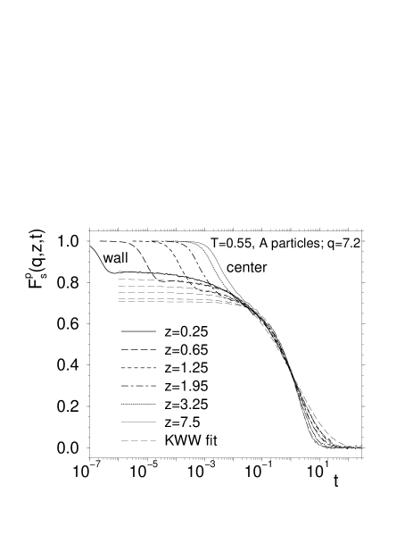
Figure 5: Time dependence of $F^{p}_{\rm s}(q,z,t)$ as a function of rescaled time $t/\tau$ (in bold). The values of $z$ are $z=0.25,0.65,1.25,1.95,3.25$, and 7.5. The thin dashed lines are fits to the data in the $\alpha-$relaxation regime with a KWW-law (see Eq. (11)).

Figure 4 shows that the typical time scale for the relaxation increases rapidly for decreasing $z$. The question arises whether it is only the time scale that depends on $z$ or whether also the shape of the curve depends on the distance from the wall. To check this we can define a relaxation time $\tau$ by requiring that at this time the correlator has decayed to $1/e$ (see horizontal dashed line in Fig. 4). In Fig. 5 we show a plot of $F^{p}_{\rm s}(q,z,t)$ vs. $t/\tau$ for various values of $z$. If the shape of the curves would be independent of $z$ we would find that this rescaling of time produces a master curve. However, from the figure we see that this is not the case since the correlators for small values of $z$ are more stretched.

In order to quantify this effect we have fitted the correlators by a Kohlrausch-Williams-Watts function (KWW),

$$F^{p}_{\rm s}(q,z,t)=f_{c}(z)\cdot\exp\left[-\left(\frac{t}{\tilde{\tau}(z)}\right)^{\beta(z)}\right]\,,$$ (11)

a functional form often used to describe the $\alpha-$relaxation of supercooled liquids. That this function is able to characterize well also the correlators in the confined liquid is demonstrated in Fig. 5 where we have included the KWW fits to the data as well (thin dashed lines).

Figure 6: $z-$dependence of the KWW parameters $f_{c}$, $\tilde{\tau}$ and $\beta$ as obtained from fits to $F^{p}_{\rm s}(q,z,t)$ for $T=0.7$ (thin lines) and $T=0.55$ (bold lines).

In Fig. 6 we show the $z-$dependence of the fit parameters obtained by fitting $F^{p}_{\rm s}(q,z,t)$ with a KWW function. The two set of curves correspond to $T=0.7$ and $T=0.55$ (thin and bold lines, respectively). We start the discussion with the relaxation times $\tilde{\tau}$ (dashed lines in the figure). From the figure it becomes clear that for large $z$ this relaxation time is basically independent of $z$ and is the same as the one found in the bulk. For decreasing $z$ it starts to rise rapidly and at the smallest $z$ for which we were able to determine it, it is more than two decades higher than the bulk value. The parameter $f_{c}$, i.e. the height of the plateau in the $\beta-$relaxation regime, shows only a relatively mild $z-$dependence in that it increases by about 20% in the $z-$range considered (dotted curves). In contrast to this, the third parameter of the KWW-function, the stretching parameter $\beta$, shows a relatively strong $z-$dependence in that it decreases from a value around 0.8 to $\beta\approx 0.33$ at small $z$. Thus we see that not only do the relaxation times increase with decreasing $z$, but that also the stretching increases significantly. The likely reason for this strong stretching is that very close to the surface the system is very heterogeneous in the sense that a slight modification of the local (frozen) environment, and such variations are certainly present, will give rise to very strong fluctuations in the relaxation behavior. Hence if one averages over these fluctuations the result is a very pronounced stretching. Note that this small value of $\beta$ is also the reason why the correlators for small $z$ decay by 4-5 orders of magnitude slower than the ones at large $z$ (see Fig. 4), whereas the relaxation time $\tilde{\tau}$ increases only by a factor of $10^{2}$.

A comparison of the data sets for $T=0.7$ and $T=0.55$ shows that the $z-$dependence for $f_{c}$ and $\beta$ are, within the noise of the data, the same. This implies that also for the confined system the so-called time-temperature superposition is valid, i.e. that the shape of the curves is independent of temperature. This feature is often found in glass forming liquids and in particular also for the present binary Lennard-Jones system kob95b . However, we already point out at this place that the relaxation times for the two temperatures do not differ by just a constant factor. We will come back to this point in Sec. III.3.

III.2 Factorization property of generalized correlation functions

Since the relaxation dynamics of the present Lennard-Jones system in the bulk is described well by means of mode-coupling theory, we will try to test to what extend some of the predictions of this theory hold for our confined systems. We have already seen that for a given value of $z$ the time-temperature superposition principle holds, in agreement with the prediction of MCT. A further important prediction of the theory is the so-called factorization property for the $\beta-$relaxation: Consider any correlator $\Phi_{x}(t)$, where $x$ stands for wave-vector, particle species, etc. MCT predicts that in the time window of the $\beta-$regime the time dependence of $\Phi_{x}(t)$ can be written as follows:

$$\Phi_{x}(t)=f^{\rm c}_{x}+h_{x}G(t)\,.$$ (12)

Here $f^{\rm c}_{x}$ and $h_{x}$ are the height of the plateau and an amplitude, respectively. The remarkable statement of MCT is that the whole time and $T-$dependence of the correlator is given by the function $G(t)$, the so-called $\beta-$correlator, and that this function is system universal, i.e. it does not depend on $x$.

One possibility to check whether or not the factorization property holds is to calculate the following function signorini90 :

$$R_{x}(t)=\frac{\Phi_{x}(t)-\Phi_{x}(t^{\prime})}{\Phi_{x}(t^{\prime\prime})-\Phi_{x}(t^{\prime})}\,,$$ (13)

where $t^{\prime}$ and $t^{\prime\prime}$ are two arbitrary times in the $\beta-$regime. If the factorization property holds, the function $R_{x}(t)$ should be independent of $x$.

For the bulk system it was found that the factorization property does indeed hold very well in that the data for $R_{x}(t)$ for all sort of different correlators do indeed fall on top of each other gleim99 . In the following we thus will check to what extend this holds also true for $z-$dependent correlators.

Figure 7: Time dependence of $F^{p}_{\rm s}(q,z,t)$ for the A particles at $T=0.55$ for different wave-vectors (see legend) for particles in the center ($7.35<z<7.5$, bold lines) and at the surface ($0<z<0.15$, thin lines).

To begin we investigate the wave-vector dependence of these functions. Figure 7 shows that qualitatively the time dependence of the correlators is independent of $q$ but that the typical relaxation time as well as the height of the plateau increases rapidly with decreasing $q$. For large values of $z$ (bold curves) and large wave-vectors it is in fact difficult to see that there is indeed a plateau (see curve for $q=18.5$) since the curve decays very quickly. This is due to the fact that large wave-vectors correspond to small displacements of the order $2\pi/q$ and that thus a decorrelation of the particle position can take place already on a very short time scale. No such fast decay is seen for small values of $z$ (thin curves) since there the relaxation dynamics is very slow even on small length scales.

Figure 8: Time dependence of the function $R(q,z,t)$ from Eq. (13) in order to test the factorization property for the incoherent intermediate scattering function $F^{p}_{\rm s}(q,z,t)$ for A particles and different values of $z$ (see main text for details). (a) $q=3.5$; (b) $q=7.2$; (c) $q=12.5$. (d) The master functions $R(q,z,t)$ for different values of $q$.

Since the factorization property is predicted to hold only in the $\beta-$relaxation regime, it is necessary that correlators show a well developed plateau. From Fig. 7 we recognize that at $T=0.55$ this condition is not fulfilled for large values of $z$ and therefore it is not possible to check whether or not the factorization property holds. However, since these correlators are very similar to the one in the bulk, and it has been shown that for the bulk system the factorization property holds gleim99 , we can assume that it does so also for the confined system at large $z$, if the temperature is sufficiently low. For small values of $z$ it is instead possible to make a direct check on the validity of the factorization property by calculating the function $R_{x}(t)$. The results are presented in Fig. 8 where we show the time dependence of the function $R_{x}(t)$ for different values of $z$ (spaced by $\Delta z=0.075$) and three different wave-vectors (panels (a)-(c)). The times used were $t^{\prime}=7.0$ and $t^{\prime\prime}=3000$. We recognize that in the $\beta-$regime the correlators for the different values of $z$ fall nicely onto a master curve, thus showing that the factorization property holds. Note that the fact that these curves fan out at short and long times shows that the existence of such a master curve is by no means a trivial matter.

The existence of the master curves shown in Figs. 8a-c demonstrates that the shape of the correlators is independent of $z$, as predicted by MCT. However, this shape should also be independent of $q$. In order to check this prediction we have calculated for several values of $q$ a mean master curve by averaging the correlator $F^{p}_{\rm s}(q,z,t)$ over $0<z<0.75$. The time dependence of these master curves for the different wave-vectors are shown in Fig. 8d. From this figure we see that the shape of the master curve does depend on $q$, i.e. the factorization property does not hold. It might of course be that the factorization property does hold at even lower temperatures, but due to the finite size effects discussed in Sec. III.6 this can presently not be checked.

III.3 Structural relaxation times

Figure 9: $z$-dependence of relaxation times $\tau_{q}(z)$ from $F^{p}_{\rm s}(q,z,\tau_{q})=1/e$ at different temperatures (see legend in part (a)). (a) Log-lin plot of the data. The open diamonds at $z=7.5$ are the relaxation times in the bulk; (b) Reduced plot of $\tau_{q}$ versus $[z-z_{\rm p}]^{-1}$ with $z_{\rm p}=-0.5$. The horizontal lines are the bulk values of $\tau_{q}$. (c) Plot of $\log[\tau_{q}(z)/\tau_{0}]$ versus $z$ with $\tau_{0}$ as a temperature dependent parameter. See main text for details.

We will now discuss in more detail the spatial dependence of structural relaxation times in the liquid. In Fig. 9a we plot $\tau_{q}(z)$, defined by $F^{p}_{\rm s}(q,z,\tau_{q})=1/e$, for all temperatures investigated. From this graph we recognize that the thickness of the film is sufficiently large since at all temperatures the relaxation times become independent of $z$ and are very close to the value in the bulk (open diamonds at $z=7.5$). At the highest temperature bulk behavior is realized already for $z\approx 2.0$. With decreasing temperature the influence of the wall reaches further into the system, i.e., the region which is affected by the wall grows with decreasing temperature and at the lowest temperature considered it extends up to $z\approx 5.0$. From the plot it also becomes evident that if the temperature would be decreased somewhat more, the relaxation times in the middle of the film would no longer coincide with the ones of the bulk, i.e. that $\tau_{q}(z)$ becomes a function of $D$.

Our main goal is now to extract a characteristic dynamic length scale from the data. Since there are no reliable theoretical concepts on how this should be done, we are forced to use just an empirical description of our data which includes such a length scale. In simulations of the same Lennard-Jones liquid within a narrow cylindrical pore scheidler00 we have been able to find such a description, at least for the particles close to the walls, i.e. for small $z$. The proposed Ansatz had the form

$$\tau_{q}(z)=f_{q}(T)\exp[\Delta_{q}/(z-z_{\rm p})]\,,$$ (14)

where $z_{\rm p}$ is a fit parameter that gives some sort of “penetration depth” of the particles into the wall scheidler00 . That this functional form is indeed able to describe the data very well is shown in Fig. 9b. The solid inclined lines are fits with the function given by Eq. (14) and we have chosen $z_{\rm p}=-0.5$. Since the slope of these lines are the parameter $\Delta_{q}$, we see that this quantity is increasing with decreasing temperature (from 2.8 at $T=2.0$ to 7.5 at $T=0.5$). We note that this result is in contrast to the one found for the narrow pore in that there we found that the fit works well even if $\Delta_{q}$ and $z_{\rm p}$ are kept constant, i.e. independent of $T$ scheidler00 . The reason for this difference might be that in Ref. scheidler00 the temperature at which the wall was frozen was always the same, in contrast to the present case where $T_{\rm W}$ is set equal to $T$, see Sec. II. (We remark that it is also possible to obtain good fits to the data by keeping $\Delta_{q}$ fixed to 7.53 and to make $z_{\rm p}$ depend on temperature scheidler_diss .)

We now extract a characteristic length scale for the influence of the wall by determining the length at which the fit with Eq. (14) crosses the bulk value (horizontal lines in Fig. 9b). In the following we will denote this so determined length scale by $\tilde{z}$ and in the next subsection we will discuss its $T-$dependence. (We remark that the values of $\tilde{z}$ depend only weakly on the way one does the fit to the data with Eq. (14), i.e. whether $\Delta_{q}$ or whether $z_{\rm p}$ is kept constant.)

Since Eq. (14) is only capable to describe the data close to the wall we looked for alternative possibilities to parameterize the relaxation times. If one thinks of a characteristic length scale $\xi_{0}$ for a decay process, a natural Ansatz is the exponential form $\exp[-z/\xi_{0}]$. However, an analysis of the difference of $\tau_{q}(z)$ to the bulk value showed that the increase is much stronger than purely exponential, and therefore we made an exponential Ansatz for the logarithm of the ratio between $\tau_{q}(z)$ and a reference value $\tau_{0}$:

$$\ln\left[\frac{\tau_{q}(z)}{\tau_{0}}\right]=A(T)\cdot\exp\left[-\frac{z}{\xi_{0}(T)}\right]\,.$$ (15)

In an ideal situation $\tau_{0}$ should of course correspond to the bulk value since for large distances from the wall we have $\tau_{q}(z)=\tau_{q}({\rm bulk})$. However, remaining small density differences within the simulation as well as finite size effects (see section III.6) lead to small deviation from this theoretical value. Hence it was possible to improve the fit, in particular close to the surface where the $z$-dependence is most pronounced, by extracting $\tau_{0}$ from an extrapolation of $\tau_{q}(z)$ to large $z$ or by using $\tau_{0}$ as a free parameter. This was done to obtain the data shown in Fig. 9c, where we plot in a logarithmic way the left hand side of Eq.(15) as a function of $z$. (We mention that the values for $\tau_{0}$ differ only slightly from the bulk values.) We see that the data are indeed compatible with straight lines, and this for all distances, thus validating the Ansatz. The negative of the slope of the straight lines is the inverse of $\xi_{0}$ and from the fact that this slope decreases with decreasing temperature we see that $\xi_{0}$ becomes larger if $T$ is lowered. In the next section we will discuss the $T-$dependence of $\xi_{0}$ in more detail. Finally we mention that the length $\xi_{0}$ decreases slightly with increasing wave-number $q$, but that this effect is only weak scheidler_diss .

Figure 10: Fit of the simulation data for $F^{p}_{\rm s}(q,z,t)$ for A particles at $q=7.2$ and $T=0.55$ according to Eq. (16) for several values of $z$ ($z=0.1,$ 0.3, 0.5, 0.7, 1.0, 1.5, 2.0, 3.0, and 7.5).

In Ref. scheidler02b we attempted not only to describe the $z-$dependence of the relaxation times but the whole time and space dependence of the scattering function $F^{p}_{\rm s}(q,z,t)$. The Ansatz used in that study had the following form:

$$F^{p}_{\rm s}(q,z,t)=F_{\rm s}^{\rm bulk}(q,t)+a(t)\exp\left[-\left(z/\xi(t)\right)^{\beta(t)}\right]\,.$$ (16)

Here $F_{\rm s}^{\rm bulk}(q,t)$ is the intermediate scattering function in the bulk and thus the second term of the left hand side of Eq. (16) describes the deviation of $F^{p}_{\rm s}(q,z,t)$ from this correlator. That this type of Ansatz is able to give a very good description of the time dependent data is demonstrated in Fig. 10 where we show $F^{p}_{\rm s}(q,z,t)$ for different values of $z$ (symbols) and the corresponding fit (dashed lines. (We mention that if one plots the data versus $z$ for different times $t$ the agreement between data and fit is very good as well (see Ref. scheidler02b ).)

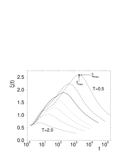
Figure 11: Time and temperature dependence of the fit parameter $\xi(t)$ from Eq. (16) at different temperatures ($T=2.0,$ 1.0, 0.8, 0.7, 0.6, 0.55, and $0.5$).

The time and $T-$dependence of the stretching parameter $\beta(t)$ is discussed in Ref. scheidler02b . Here we focus on the dependence of the length scale $\xi(t)$ on $t$ and $T$. This dependence is shown in Fig. 11 from which we recognize that $\xi(t)$ is a smooth function of time with a local maximum $\xi_{\rm max}$ at $t=t_{\rm max}$. The location of this maximum shifts to larger times if $T$ is decreased and also its value increases.

Thus we conclude that there exists a characteristic time scale at which the influence of the wall extends farthest into the liquid, i.e. for which the system is relatively stiff. This time scale corresponds roughly to the time of the $\alpha$-relaxation in the bulk system scheidler_diss , a result which is plausible as can be seen as follows: It is well known that for simple liquids the $\alpha-$relaxation is largest for wave-vectors at the peak of the static structure factor (see, e.g., data in Ref. kob95b ), i.e. the length scale that corresponds to the typical distance between the particles. Since it is this time scale which is really relevant for the structural relaxation, since it corresponds to the typical time needed for the particles to leave their cage, it can be expected that any external perturbation, such as the presence of the wall, will affect the dynamics at long distances on this time scale which is comparable with this relaxation time.

Finally we remark that the qualitative behavior as well as the height of the maximum in $\xi(t)$ does not change significantly if one fits the data with an exponential function, i.e. $\beta(t)\equiv 1$ in Eq. (16), (see the subsequent section and Fig. 12), although we note that such a fit is not able to describe the data very well scheidler_diss .

III.4 Dynamic length scales

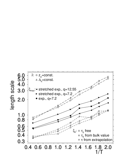
Figure 12: Comparison of different dynamic length scales as extracted from the spatial dependence of scattering functions $F^{p}_{\rm s}(q,z,t)$ and structural relaxation times: $\tilde{z}$ from fits with Eq. (14), $\xi_{0}$ from fits with Eq. (15) and $\xi_{\rm max}$ from fits with Eq. (16) (see also legend and text).

From the results described so far we were able to extract three different dynamic length scales: $\tilde{z}$ from Eq. (14), $\xi_{0}$ from Eq. (15), and $\xi_{\rm max}$ from the Ansatz given by Eq. (16). We now discuss how these different length scales depend on temperature. This $T-$dependence is shown in Fig. 12 where we have plotted $\tilde{z}$, $\xi_{0}$, and $\xi_{\rm max}$ as a function of inverse temperature. First of all we recognize that the different definition of length scale give basically all the same result and that thus the precise definition is not relevant. Furthermore we see that it is also not crucial how exactly one defines a length scale: For the case of $\tilde{z}$ it does not manner whether one keeps $\Delta_{q}$ or $z_{\rm p}$ independent of $T$ (see discussion of Eq. (14)); for the case of $\xi_{0}$ it does not matter whether the relaxation time $\tau_{0}$ is the bulk value, the value obtained from extrapolating $\tau_{q}(z)$ to large $z$, or whether it is just a fit parameter; for the case of $\xi_{\rm max}$ it is irrelevant at which wave-vector one uses the Ansatz (16) or whether $\beta(t)$ is set to unity or not.

Note that we have plotted all data in an Arrhenius plot, i.e. logarithmically versus inverse temperature. Although to our knowledge there is no theoretical reason why one should plot the data in this manner, the graph shows that this presentation does rectify the data. Thus we conclude that the length increases like $\exp(B/T)$ and that the value of $B\approx 1.2$ is independent of the length scale. In Ref. scheidler02a we have discussed the temperature dependence in more detail and made also a comparison with other characteristic length scales in the liquid. The conclusion is that basically all relevant length scales are very similar in size and show a quite similar $T-$dependence. Finally we remark that this $T-$dependence is significantly larger than the one that one obtains from the one of static quantities like, e.g., the envelope of the radial distribution function scheidler02a .

III.5 Collective quantities

To get a better understanding of the collective dynamics close to the surface we investigate the intermediate scattering function $F(q,z,t)$ for all (A and B) particles which is given by Eq. (9). In this quantity the initial position of a particle is correlated with the position of any other particle at a later time $t$. The main consequence for the behavior close to the surface is the following. Since the configuration of the wall particles is frozen there exist a static landscape in the potential energy and particles of the liquid prefer to occupy the local minima in this landscape. Therefore it can be expected that as soon as a liquid particle close to the surface leaves its position this vacancy will be filled by another particle. This implies that the collective correlation function close to the wall does not decay to zero even at long times.

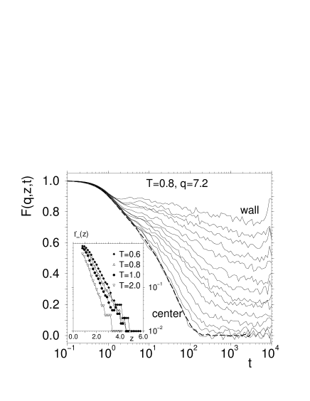
Figure 13: Normalized coherent intermediate scattering function $F(q,z,t)$ for $q=7.2$ for both types of particles at $T=0.8$. The thin curves correspond to $z=0.3,0.45,0.6,\ldots,1.35,1.5,1.8,2.25,2.85,3.9,7.5$. The bold dashed line is the data for the bulk. Inset: $z-$dependence of the height of the plateau $f_{\infty}(z)$ for different temperatures.

That this expectation is indeed met is shown in Fig. 13 where we plot the time dependence of $F(q,z,t)$ as a function of temperature. Note that, in order to improve the statistics of the data, we do not distinguish between A and B particles and in addition we have made a spherical average. We mention, however, that the data in which we averaged only over wave-vectors parallel to the surfaces look qualitatively quite similar scheidler_diss .

Also included in the figure is the corresponding correlator for the bulk system (bold dashed line) and we recognize that this function coincides with $F(q,z,t)$ for large values of $z$. Furthermore we see that the height of the plateau in $F(q,z,t)$ at long times increases rapidly with decreasing $z$ and that for the smallest $z$ we do no longer find the two-step relaxation usually seen in supercooled liquids. The $z-$dependence of the height of this plateau, $f_{\infty}(z)$, is shown in the Inset of the figure (in a log-lin plot). We see that it shows basically an exponential decay, although within the noise of the data it is difficult to exclude other functional forms. The slope of the straight lines in the Inset gives a static length scale over which the liquid starts to become uncorrelated with the “pinning-field” generated by the wall. Thus it can be expected that this length scale is comparable to the one found in other static two-point correlation functions, such as, e.g. the decay of the correlation in the radial distribution function. In agreement with this expectation we see that this length scale is indeed on the order or 2-3 and that it shows only a weak dependence on temperature. In particular this $T-$dependence is significantly weaker than the one found for the dynamical length scales discussed above.

Due to the presence of the plateau at long times in $F(q,z,t)$, it is difficult to extract a relaxation time from this function. In an attempt to define such a time scale, we have subtracted the long time limit of $F(q,z,t)$ and normalized the function by $1-f_{\infty}(z)$. For the so obtained resulting normalized correlator it is possible to define a relaxation time. However, we have found that this time scale depends only relatively weakly on $z$, and in particularly much weaker than the relaxation time for $F_{s}^{p}(q,t,z)$, and therefore this approach was no longer pursued scheidler_diss .

III.6 Films with a finite thickness

Until now we have considered only values of $D$ and $T$ such that the system under investigation is sufficiently large to guarantee that in the center it has the same dynamics as in the bulk. Thus strictly speaking we have so far only investigated the dynamics of a liquid in the vicinity of one wall and the fact that the overall geometry is a film was completely irrelevant. However, from Fig. 9 we have concluded that with decreasing temperature the dynamical length scales for cooperativity are growing and that the influence of the wall reaches further into the system. Therefore it is obvious that for a system of a given thickness also the particles in the center will be influenced by the walls, if the temperature is sufficiently low. Hence it can be expected that the dynamics should be slowed down even more and the goal of this subsection is to investigate this effect in more detail.

Figure 14: Local relaxation times in films with different thickness ($D=15.0,$ 10.0, and 5.0). Plot of the left hand side of Eq. (15) versus distance to the nearest wall (symbols). The lines correspond to the Ansatz given by Eq. (15) with parameter that have been determined in systems with $D=15.0$.

Instead of lowering the temperature we investigate films that have a smaller thickness ($D=10.0$ and $D=5.0$) for temperatures down to $T=0.6$. We have repeated the procedure described in the previous subsection for $D=15.0$ in order to obtain the $z-$dependence of the relaxation times of the incoherent intermediate scattering function and we present this dependence in Fig. 14. At high temperatures, where each particle is influence by at most one wall, the local dynamics is only a function of its distance to the wall. This can be see by the data for $T=2.0$ since the curves for the different values of $D$ fall on top of each other and can, e.g., be described by the exponential Ansatz of Eq. (15), solid line. If we decrease temperature, $T=0.8$, the data for the thinnest film starts to deviate from the master curve because the particles in the center already feel the presence of both walls. At even lower temperatures, $T=0.6$, this effect becomes more pronounced and also the data for $D=10.0$ starts to deviate from the one of $D=15.0$. Note that since at this $T$ the data for $D=10.0$ shows strong deviations from the one for $D=15.0$ at $z=5.0$, it follows that in a film of thickness $D=5.0$ the particles close to a wall are also influenced by the presence of the opposite wall.

The question is now if this enhancement of the slowing down is just a linear effect, i.e. it is given by the sum of the contributions from both walls, or if the situation is more complicated. Under the assumption that the local dynamics at a distance $z$ from a rough surface is given by Eq. (15) a reasonable generalization is given by the Ansatz

$$\ln\left[\frac{\tau_{q}(z)}{\tau_{0}}\right]=A(T)\cdot\left\{\exp\left[-\frac{z}{\xi_{0}(T)}\right]+\exp\left[-\frac{D-z}{\xi_{0}(T)}\right]\right\}\,.$$ (17)

Using the parameters $A(T)$ and $\xi_{0}(T)$ as determined from the fits to the data for $D=15.0$, see Sec. III.3, we thus can use this expression to calculate the $z-$dependence of $\tau_{q}$ for the smaller films. The resulting predictions for $D=10.0$ and $D=5.0$ are included in Fig. 14 as well (dashed and dotted lines). We see that although the predicted curves look qualitatively similar to the data for these films, they severely underestimate the relaxation times at large values of $z$. Qualitatively the same result is obtained if we use Eqs. (14) or (16) to predict $\tau_{q}(z)$ for thin films scheidler_diss . Hence we conclude that the presence of two walls affects the relaxation dynamics of the liquid particles in a non-additive manner, i.e. that the reason for the slowing down must be non-linear. This result is not that surprising since mode-coupling theory, a very successful theoretical framework to describe the slowing down of the dynamics of glass-forming systems, predicts that this slowing down is related to a non-linear feedback mechanism mct . According to MCT the relaxation dynamics of a particle is strongly coupled to the motion of its neighboring particles that form the cage of the tagged particle. Since this tagged particle itself is part of the cage of other particles, a decrease in $T$, i.e. a stronger coupling of the motion, leads to a strong (i.e. non-linear) stiffening of the cage (feedback effect). In our case the particles that form the wall are completely frozen and thus they do no longer participate to help to relax the fluid particles in their neighborhood. Thus from a qualitative point of view the lack of fluctuations of the cage of the particles near the walls explains the slowing down of their dynamics and the feedback effect rationalizes why the presence of two walls affects the system stronger than just the linear sum of two individual walls. Finally we mention that this non-linear feedback effect should affect the relaxation dynamics even more in the case of systems in which the confinement is given by a tubular geometries or in cavities.

III.7 Mean relaxation dynamics

Having characterized in great detail the local dynamics and understood how the structural relaxation depends on the distance from the wall, we now can investigate the dynamic properties of the whole system, i.e. if one averages the correlators over $z$. These averaged correlation functions are exactly the quantities that are accessible in most experiments. In contrast to experiments we are, however, in the favorable position to be able to relate these averaged quantities to the time dependence of the local ones.

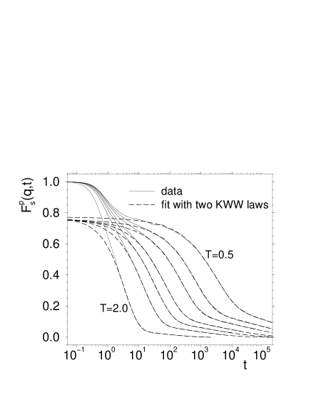
Figure 15: Self part $F^{p}_{\rm s}(t)$ of the intermediate scattering function for A particles in a film with $D=15.0$ for $q=7.2$ and temperatures $T=2.0,1.0,0.8,0.7,0.6,0.55$, and $0.5$ (solid lines). The dashed lines are fits to the data with a superposition of two stretched exponential laws.

In Fig. 15 we show the time dependence of $F^{p}_{\rm s}(q,t)$, i.e. the incoherent intermediate scattering function for the A particles averaged over the whole film (solid lines). (The wave-vector is again parallel to the walls.) Although at a first glance these correlators look quite similar to the ones in the bulk kob95b , a closer inspection shows that there are important differences. Already at $T=2.0$ one sees that after a rapid decay to a small value around 0.05, the correlator shows a tail that extends to relatively long times. At low temperatures the function shows at intermediate times the usual plateau that is related to the cage effect but at longer times the mentioned tail starts now to become very pronounced.

The reason for this behavior follows directly from the results of the local correlation functions. Since the typical time scales for the structural relaxation as a function of $z$ extend over several decades in time, the average over all those curves should be very stretched (see also Fig. 4). For $T=2.0$ particles with $z>2.0$, i.e. more than 70% of the particles, behave more or less bulk-like and contribute to the fast decay seen in Fig. 15 at short times. The correlators for particles at the surface decay much slower and give therefore rise to the long time tail for $t>10$. With decreasing temperature the number of particles with a relaxation that is significantly slower than the one in the bulk becomes larger and therefore the amplitude of the long time tail increases. As a consequence the shape of the correlators change with temperature, i.e. the time-temperature superposition principle is not valid, in contrast to the case of the bulk system kob95b . Therefore the definition of characteristic relaxation times for the whole decay is not really possible.

Of course one can calculate the time dependence of $F^{p}_{\rm s}(q,t)$ from the knowledge of the $z-$dependent correlators which we are able to describe by a set of KWW functions (see Fig. 5). On the other hand, in experiments this information is usually not available and therefore it is interesting to check how one can characterize the averaged data in a different way. We have found that for all temperatures considered, the $\alpha-$relaxation of the average correlator can be described very well by the sum of two KWW-laws (having different amplitudes): One that is for the early part of the relaxation and the second one for the mentioned tail. That this type of Ansatz does indeed give a very good description of the data is shown in Fig. 15 where we have included the results of such fits as well (dashed lines).

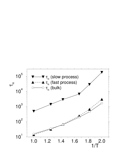
Figure 16: Temperature dependence of the relaxation times of the two processes extracted from the self part of the intermediate scattering function averaged over all A particles in the system (filled triangles). The open circles are the $\alpha-$relaxation time for the bulk.

In Fig. 16 we show the temperature dependence of the relaxation times, obtained from the KWW fits, for the fast and slow process. We see that within the accuracy of the data i) these $T-$dependencies are very similar, although the time scale for the slow process is around 40 times larger, and ii) that the fast process shows basically the same $T-$dependence as the bulk system. For the fast process the values for the KWW-parameter $\beta$ is around 0.8 and depends only weakly on $T$. In contrast to this we find for the slow process that $\beta$ is only around 0.25-0.3, i.e. a very small value scheidler_diss . The reason for such a strong stretching, which is basically independent of $T$, is that the relaxation dynamics is extremely heterogeneous, i.e. that close to the wall the typical time scales differ by orders of magnitude (see Fig. 4).

Thus we find that the long time tail is basically given by the second process which has a clearly separated time scale with a smaller amplitude. Note that this conclusion comes from our data in the time domain. However, it is also possible to make a time-Fourier transform of our data and to calculate the dynamical susceptibility $\chi(\omega)$. This has been done in Ref. scheidler02a where it was shown that these two processes can also be seen in the frequency domain in that one finds that the imaginary part of $\chi(\omega)$ seems to be indeed the sum of two peaks. Such a double peak structure is often found in real spectroscopy experiments where one observes a second peak at frequencies well below the peak corresponding to the $\alpha-$relaxation of the bulk system. Thus from such averaged data one could easily come to the conclusion that there are indeed two distinct processes, e.g. one corresponding to particles in the center and the other to a layer of slow particles at the surface and which give rise to the second process. However, the analysis of the $z-$dependent correlators presented here shows that such a conclusion might be wrong.

Figure 17: Time dependence of the intermediate scattering function $F^{p}_{\rm s}(q,t)$ for all A particles in films with different thickness ($D=15.0$, 10.0, 5.0) for $q=7.2$ and different temperatures ($T=2.0$, 0.8, 0.55). The dotted curves correspond to the bulk data.

Finally we discuss how the averaged time correlation function depends on the thickness of the film. In Fig. 17 we show $F^{p}_{\rm s}(q,t)$ for different temperatures and three values of $D$ as well as for the bulk system. We see that in these averaged curves one can notice already at the highest temperature a significant deviation of the correlators for the confined systems from the one of the bulk. This is due to the presence of the particles that are slowed down near one of the walls. (Recall that in Fig. 14 we have seen that at this $T$ none of the particles of even the smallest system are affected by both walls.) Thus the amplitude of the tail at long times is given only by twice the fraction of the particles that are strongly affected by one wall. (Note that the value of this fraction depends on $D$.) With decreasing $T$ the fraction of particles affected by one wall increases, due to the growing dynamical length scale and hence the curves for the confined system decay significantly slower than the bulk curves. For even lower temperatures we have the additional effect that the particles close to the center are affected in a non-linear way by the presence of both walls, which leads to an additional slowing down. Thus we see that the $T-$ and $D-$dependence of the relaxation function is quite complex since there are three main causes: i) The general slowing down of the dynamics with decreasing temperature; ii) The presence of a growing length scale over which the slow dynamics close to the wall affects the relaxation dynamics; iii) The non-linear effects occurring if a particle is influenced by more than one wall. The sum of these causes has the effect that the shape of the correlation function depend in a strong and highly non-trivial way on $T$ and $D$. This dependence also hampers a sensible definition of a relaxation time which is the reason why we do not discuss the $T-$ and $D-$dependence of it.

IV Summary and conclusion

In this paper we have presented the results of a molecular dynamics computer simulation of a binary Lennard-Jones liquid confined between two rough surfaces. The walls are given by a frozen amorphous configuration of the same liquid and as we have shown here that the static properties of the confined fluid are identical to the ones of the bulk system. We have found that the relaxation dynamics of particles close to the interface are slowed down by orders of magnitude with respect to the one in the bulk. Due to the cooperativity of the particle motion within a liquid, also particles at some distance from the wall are influenced by the presence of the wall. Therefore the properties of the structural relaxation become a function of distance $z$ to the wall. All these properties are a smooth function of $z$, although some of them show a very strong $z-$dependence which results that the dynamics of the system is very heterogeneous.

The time dependence of the incoherent intermediate scattering functions $F_{\rm s}(q,z,t)$ is described well by a KWW-function with a stretching parameter $\beta$ and a relaxation time $\tilde{\tau}$ that depends strongly on $z$. The $z-$dependence of the relaxation times can be described well by various phenomenological laws. From these laws it is possible to extract various dynamical length scales over which the dynamics of the system is influenced by the walls.

These length scales are of purely dynamical origin and show a $T-$dependence which is compatible with an Arrhenius law with an activation energy that is independent of the details of the definition of the length scale. Note that this $T-$dependence is in contrast to other dynamical length scales that have been discussed in the literature before, such as, e.g., the dynamical heterogeneities donati99a ; franz99 ; franz00 for which a divergence at a temperature close to $T_{c}$ of mode-coupling theory has been found. We have tested whether or not the $T-$dependence of our length scales are compatible with a divergence at a finite temperature and have found, see Ref. scheidler_diss , that in principle such a scenario is possible at $T_{c}$ or at $T_{K}$, the Kauzmann temperature of the system. However, the noise in the data is unfortunately too large to make strong statements on this point.

As long as the dynamical length scales are significantly smaller than the system size, the discussed results are just an effect due to the interface, i.e. the dynamics is only a function of distance to the surface and independent of the film thickness. For a film with given thickness there exists however a threshold temperature below of which particles are influenced by both interfaces since the size of the CRR’s are larger than $D/2$. In that case we find that the slowing down is much stronger than one might expect from a simple linear superposition of the influence of two single surfaces. This is evidence that the mechanism for the slowing down of the particles is a strongly non-linear effect, such as proposed, e.g., by mode-coupling theory.

Finally we have studied the time dependence of the correlators averaged over the whole film. These correlators are a quite complex function of $T$ and $D$ since one has to distinguish between the normal slowing down of the liquid with decreasing temperature (which is present in the bulk system as well), the influence of one interface on the dynamics with a dynamical length scale that increases with decreasing $T$, and last not least with the mentioned non-linear effects. In view of these different reasons for the slowing down of the average dynamics, it is clear that it is rather difficult to come up with an expression for the $D-$dependence of the glass transition temperature, since it is not even obvious how the typical relaxation time of the system should be defined.

Despite this uncertainty it is clear that the glass transition temperature, which could be defined as the temperature at which a relaxation time or the viscosity attains a given predescribed value, will increase with decreasing thickness of the film. However, we point out that this qualitative result holds only true for the case of rough walls as they have been considered in the present work. In a different study we have also investigated the relaxation dynamics of a system with smooth walls where we have again made sure that the structural properties of the confined liquid is not changed by these interfaces scheidler_diss ; scheidler02a . In that study we have found that the dynamics close to the wall is accelerated which in turn leads to a decrease of the glass transition temperature with decreasing $D$. Hence we conclude that the relaxation dynamics is strongly affected by the nature of the confining walls, in agreement with experimental results. Thus it seems that it would be of interest to avoid these confining walls altogether in order to disentangle the influence of the wall on the dynamics and the effect of the finite extension of the system. Within a simulation this is indeed possible since one can investigate the relaxation dynamics of a given system for different system size (using periodic boundary conditions in all three directions). In the past such simulations have been done and it has been found that at a given temperature the relaxation dynamics slows down with decreasing temperature buchner99 ; kim00 . Hence we conclude that intrinsically confinement leads to a slower dynamics but that the presence of fluid-wall interactions can completely mask this general trend.

Last not least we comment on the necessity for a more complete theoretical understanding of the relaxation dynamics of confined systems. The present simulations have shown that it is possible to have a slowing down of the dynamics without a change of the structural properties (and in Refs. scheidler03 ; scheidler02a it was shown that also an acceleration can be observed). Hence we conclude that it is not sufficient to know the structure in order to predict the dynamics. This is in contrast to the situation of the bulk where it is indeed possible, using mode-coupling theory, to predict the relaxation dynamics using as input only structural quantities mct ; kob02 . For the moment it is not clear to us how this theory has to be modified in order to rationalize the results found in this work. Of course it is probably possible to use some phenomenological theories in order to describe these results herminghaus01 ; long01 ; mccoy02 but having a theory at hand that allows a full microscopic calculation would certainly be much more preferable.

Acknowledgement: Part of this work was supported by the DFG under SFB 262, by the European Community’s Human Potential Programme under contract HPRN-CT-2002-00307, DYGLAGEMEM, and the NIC in Jülich.

References

- (1) K. L. Ngai (Ed.): Proceedings of the Forth International Discussion Meeting on Relaxations in Complex Systems, Non-Cryst. Solids 307-310 (2002).
- (2) D. Turnbull and M. H. Cohen, J. Chem. Phys. 29, 1049 (1958).
- (3) G. Adam and J. H. Gibbs, J. Chem. Phys. 43, 139 (1965).
- (4) J. H. Gibbs and E. A. DiMarzio, J. Chem. Phys. 28, 373 (1958).
- (5) W. Götze, p. 287 in Liquids, Freezing and the Glass Transition Eds.: J. P. Hansen, D. Levesque, and J. Zinn-Justin, Les Houches. Session LI, 1989, (North-Holland, Amsterdam, 1991); W. Götze, J. Phys.: Condens. Matter 10, A1 (1999).
- (6) W. Kauzmann, Chem. Rev. 43, 219 (1948).
- (7) L. Sjögren, Phys. Rev. A 22, 2866 (1980).
- (8) E. Donth, Relaxation Dynamics in Liquids and Disorders Materials (Springer, Berlin, 2001).
- (9) H. Rieger, p. 295 in Vol. II of Annual Reviews of Computational Physics, Ed.: D. Stauffer (World Scientific, Singapore, 1995).
- (10) L. Berthier, Phys. Rev. Lett. 91, 055701 (2003).
- (11) C. Donati, J. F. Douglas, W. Kob, S. J. Plimpton, P. H. Poole, and S. C. Glotzer, Phys. Rev. Lett. 80, 2338 (1998).
- (12) B. Doliwa and A. Heuer, Phys. Rev. E 61, 6898 (2000).
- (13) E. R. Weeks, J. R. Crocker, A. C. Levitt, A. Schofield, and D. A. Weitz, Science 287, 627 (2000).
- (14) W. K. Kegel and A. van Blaaderen, Science 287, 290 (2000).
- (15) C. Donati, S. C. Glotzer, and P. H. Poole, Phys. Rev. Lett. 82, 5064 (1999).
- (16) J. M. Drake, J. Klafter, R. Kopelman, and D. D. Awschalom, Dynamics in Small Confining Systems Mater. Res. Soc. Proc. Vol. 290 (MRS, Pittsburg, 1993)
- (17) J .M. Drake, J. Klafter, P. Levitz, R. M. Overney, and M. Urbakh, Dynamics in Small Confining Systems V Mater. Res. Soc. Proc. Vol. 651 (MRS, Pittsburg, 2001)
- (18) B. Frick, R. Zorn, and H. Büttner, Proceedings of International Workshop on Dynamics in Confinement J. Phys. France IV 10, Pr7 (2000).
- (19) J. A. Forrest and K. Dalnoki-Veress, Adv. Coll. Interf. Science 94, 167 (2001).
- (20) B. Frick, M. Koza, and R. Zorn, Proceedings of Second International Workshop on Dynamics in Confinement Eur. Phys. J. E (2003).
- (21) C. L. Jackson and G. B. McKenna, J. Non-Cryst. Solids 131-133, 221 (1991).
- (22) M. Arndt, R. Stannarius, H. Groothues, H. Hempel, and F. Kremer, Phys. Rev. Lett. 79, 2077 (1997).
- (23) E. Hempel, S. Vieweg, A. Huwe, K. Otto, C. Schick, and E. Donth, J. Phys. France IV 10 Pr7 79 (2000).
- (24) J. Schüller, Yu. B. Mel’nichenko, R. Richert, and E. W. Fischer, Phys. Rev. Lett. 73, 2224 (1994).
- (25) P. Pissis, D. Daoukaki-Diamanti, L. Apekis, and C. Christodoulides, J. Phys.: Condens. Matter 6, L325 (1994).
- (26) M. Arndt, R. Stannarius, W. Gorbatschow, and F. Kremer, Phys. Rev. E 54, 5377 (1996).
- (27) F. Kremer, A. Huwe, M. Arndt, P. Behrens, and W. Schwieger, J. Phys.: Condens. Matter 11, A175 (1999).
- (28) R. Bergman and J. Swenson, Nature 403, 283 (2000).
- (29) K. Fukao and Y. Miyamoto, Phys. Rev. E 61, 1743 (2000).
- (30) Yu. B. Mel’nichenko, J. Schüller, R. Richert, B. Ewen, and C.-K. Loong, J. Chem. Phys. 103, 2016 (1995).
- (31) R. Zorn, L. Hartmann, B. Frick, D. Richter, and F. Kremer, J. Non-Cryst. Solids 307–310, 547 (2002).
- (32) R. Richert, Phys. Rev. B 54, 15762 (1996).
- (33) M. Yang and R. Richert, Chem. Phys. 284, 103 (2002).
- (34) R. Richert and M. Yang, J. Phys. Chem. B 107, 895 (2003).
- (35) G. B. McKenna, J. Phys. France IV 10, Pr7, 53 (2000).
- (36) C. Streck, Yu. B. Mel’nichenko, R. Richert, B. Ewen, and C.-K. Loong, Phys. Rev. B 53, 5341 (1995).
- (37) W. E. Wallace and J. H. van Zanten, Phys. Rev. E 52, R3329 (1995).
- (38) X. Zheng, B. B. Sauer, J. G. Van Alsten, S. A. Schwarz, M. H. Rafailovich, J. Sokolov, and M. Rubinstein, Phys. Rev. Lett. 74, 407 (1995).
- (39) A. Huwe, M. Arndt, F. Kremer, C. Haggemüller, and P. Behrens, J. Chem. Phys. 107, 9699 (1997).
- (40) J. L. Keddie, R. A. L. Jones, and R. A. Cory, Europhys. Lett. 27, 59 (1994).
- (41) J. A. Forrest, K. Dalnoki-Veress, and J.R. Dutcher, Phys. Rev. E 56, 5705 (1997).
- (42) J. A. Forrest and J. Mattsson, Phys. Rev. E 61, R53 (2000).
- (43) K. Dalnoki-Veress, J. A. Forrest, C. Murray, C. Gigault, and J. R. Dutcher, Phys. Rev. E 63, 031801 (2001).
- (44) J. Schüller, R. Richert, and E. W. Fischer, Phys. Rev. B 52, 15232 (1995).
- (45) D. Morineau, Y. D. Xia, and C. Alba-Simionesco, J. Chem. Phys. 117, 8966 (2002).
- (46) I. A. Bitsanis and C. Pan, J. Chem. Phys. 99, 5520 (1993).
- (47) T. Fehr and H. Löwen, Phys. Rev. E 52, 4016 (1995).
- (48) Z. Németh and H. Löwen, Phys. Rev. E 59, 6824 (1999).
- (49) J. Delhommelle and D. J. Evans, J. Chem. Phys. 114, 6229 (2001).
- (50) R. Yamamoto and K. Kim, J. Phys. France IV 10 Pr7, 15 (2000).
- (51) F. Varnik, J. Baschnagel, and K. Binder, Phys. Rev. E 65, 021507 (2002).
- (52) D. Kranbuehl, R. Knowles, A. Hossain, and A. Gilchriest, J. Non-Cryst. Solids 307, 495 (2002).
- (53) F. Varnik, J. Baschnagel, and K. Binder, Eur. Phys. J. E 8, 175 (2002).
- (54) K. Binder, J. Baschnagel, and W. Paul, Prog. Polym. Science 28, 115 (2003).
- (55) B. Böddeker and H. Teichler, Phys. Rev. E 59, 1948 (1999).
- (56) V. Teboul and C. Alba-Simionesco, J. Phys.: Condens. Matter 14, 5699 (2002).
- (57) P. Gallo, R. Pellarin, and M. Rovere, Phys. Rev. E 67, 041202 (2003).
- (58) K. Kim, Europhys. Lett. 61, 790 (2003).
- (59) W. Kob and H. C. Andersen, Phys. Rev. E 51, 4626 (1995).
- (60) W. Kob and H. C. Andersen, Phys. Rev. E 52, 4134 (1995).
- (61) B. Coluzzi, G. Parisi, and P. Verrocchio, Phys. Rev. Lett. 84, 306 (2000).
- (62) M. Mézard and G. Parisi, J. Phys.: Condens. Matter 12, 6655 (2000).
- (63) F. Sciortino and W. Kob, Phys. Rev. Lett. 86, 648 (2001).
- (64) P. Scheidler, Ph.D. Thesis, Universität Mainz 2002.
- (65) P. Scheidler, W. Kob, and K. Binder, Europhys. Lett. 52, 277 (2000).
- (66) G. Parisi, private communication.
- (67) P. Scheidler, W. Kob, and K. Binder, Eur. Phys. J. E (in press).
- (68) J.-P. Hansen and I. R. McDonald, Theory of Simple Liquids (Academic Press, London, 1986).
- (69) J.-L. Barrat and J.-P. Hansen, Basic Concepts for Simple and Complex Liquids (Cambridge University Press, Cambridge, 2003).
- (70) J. Horbach and W. Kob, Phys. Rev. B 60, 3169 (1999).
- (71) G. F. Signorini, J.-L. Barrat, and M. L. Klein, J. Chem. Phys. 92, 1294 (1990).
- (72) T. Gleim and W. Kob, Eur. Phys. J. B 13, 83 (2000).
- (73) P. Scheidler, W. Kob, K. Binder, and G. Parisi, Phil. Mag. B 82, 283 (2002).
- (74) P. Scheidler, W. Kob, and K. Binder, Europhys. Lett. 59, 701 (2002).
- (75) S. Franz, C. Donati, G. Parisi, and S. C. Glotzer, Phil. Mag. B 79, 1827 (1999).
- (76) S. Franz and G. Parisi, J. Phys.: Condens. Matter 12, 6335 (2000).
- (77) S. Büchner and A. Heuer, Phys. Rev. E 60, 6507 (1999).
- (78) K. Kim and R. Yamamoto, Phys. Rev. E 61, R41 (2000).
- (79) W. Kob, M. Nauroth, and F. Sciortino, J. Non-Cryst. Solids 307-310, 181 (2002).
- (80) S. Herminghaus, K. Jacobs, and R. Seemann, Eur. Phys. J. E 5, 531 (2001).
- (81) D. Long and F. Lequeux, Eur. Phys. J. E 4, 371 (2001).
- (82) J. D. McCoy and J. G. Curro, J. Chem. Phys. 116, 9154 (2002).