Measurement efficiency and n-shot read out of spin qubits

Abstract

We consider electron spin qubits in quantum dots and define a measurement efficiency $e$ to characterize reliable measurements via $n$-shot read outs. We propose various implementations based on a double dot and quantum point contact (QPC) and show that the associated efficiencies $e$ vary between 50% and 100%, allowing single-shot read out in the latter case. We model the read out microscopically and derive its time dynamics in terms of a generalized master equation, calculate the QPC current and show that it allows spin read out under realistic conditions.

The read out of a qubit state is of central importance for quantum information processing NielsenChuang . In special cases, the qubit state can be determined in a single measurement, referred to as single shot read out. In general, however, the measurement needs to be performed not only once but $n$ times, where $n$ depends on the qubit, the efficiency $e$ of the measurement device, and on the tolerated inaccuracy (infidelity) $\alpha$. In the first part of this Letter, we analyze such $n$-shot read outs for general qubit implementations and derive a lower bound on $n$ in terms of $e$ and $\alpha$. We then turn to spin-based qubits and GaAs quantum dots Loss97 ; reviewQdot and analyze their $n$-shot read out based on a spin-charge conversion and charge measurement via quantum point contacts.

$n$-shot read out and measurement efficiency $e$. How many times $n$ do the preparation and measurement need to be performed until the state of the qubit is known with some given infidelity $\alpha$ ($n$-shot read out)? We consider a well-defined qubit, i.e., we take only a two-dimensional qubit Hilbert space into account and exclude leakage to other degrees of freedom. We define a set of positive operator-valued measure (POVM) operators Peres , $E_{A_{0}}=p_{0}\left.|0\rangle\right.\langle 0|+(1-p_{1})\left.|1\rangle\right.\langle 1|$ and $E_{A_{1}}=(1-p_{0})\left.|0\rangle\right.\langle 0|+p_{1}\left.|1\rangle\right.\langle 1|$, where $p_{0}$ and $p_{1}$ are probabilities. These operators describe measurements with outcomes $A_{0}$ and $A_{1}$, resp. They are positive and $E_{A_{0}}+E_{A_{1}}=1$. This model of the measurement process can be pictured as follows. First, the qubit is coupled to some other device (e.g., to a reference dot, see below). Then this coupled system is measured and thereby projected onto some internal state. That state is accessed via an external “pointer” observable $\hat{A}$ Peres (e.g., a particular charge distribution, a time-averaged current, or noise). We assume that only two measurement outcomes are possible, either $A_{0}$ or $A_{1}$, which are classically distinguishable fnUncertOutcome . For initial qubit state $\left.|0\rangle\right.$ the expectation value is ${\langle\hat{A}\rangle}_{0}=p_{0}A_{0}+(1-p_{0})A_{1}$, while for initial state $\left.|1\rangle\right.$ it is ${\langle\hat{A}\rangle}_{1}=(1-p_{1})A_{0}+p_{1}A_{1}$. Let us take an initial qubit state $\left.|0\rangle\right.$and consider a single measurement. With probability $p_{0}$, the measurement outcome is $A_{0}$ which one would interpret as “qubit was in state $\left.|0\rangle\right.$”. However, with probability $1-p_{0}$, the outcome is $A_{1}$ and one might incorrectly conclude that “qubit was in state $\left.|1\rangle\right.$”. Conversely, the initial state $\left.|1\rangle\right.$ leads with probability $p_{1}$ to $A_{1}$ and with $1-p_{1}$ to $A_{0}$. We now determine $n$ for a given $\alpha$, for a qubit either in state $\left.|0\rangle\right.$ or $\left.|1\rangle\right.$ (no superposition allowed effSuperpos ). For an accurate read out we need, roughly speaking, that ${\langle\hat{A}\rangle}_{0}$ and ${\langle\hat{A}\rangle}_{1}$ are separated by more than the sum of the corresponding standard deviations. More precisely Bosch , we consider a parameter test of a binomial distribution of the measurement outcomes, one of which is $A_{0}$ with probability $p$. The null hypothesis is that the qubit is in state $\left.|0\rangle\right.$, thus $p=p_{0}$. The alternative is a qubit in state $\left.|1\rangle\right.$, thus $p=1-p_{1}$. For sufficiently large $n$, namely $n\,p_{0,1}(1-p_{0,1})>9$, one can approximate the binomial with a normal distribution footnoteExpG . The state of the qubit can then be determined with significance level (“infidelity”) $\alpha$ for

$$n \geq z_{1-\alpha}^{2}\Big{(}\frac{1}{e}-1\Big{)},$$ (1)

$$e = \left(\sqrt{p_{0}p_{1}}-\sqrt{(1-p_{0})(1-p_{1})}\right)^{2},$$ (2)

with the quantile (critical value) $z_{1-\alpha}$ of the standard normal distribution function, $\Phi(z_{1-\alpha})=1-\alpha=\frac{1}{2}\big{[}1+\mathrm{erf}(z_{1-\alpha}/\sqrt{2})\big{]}$. We interpret $e$ as measurement efficiency. Indeed, it is a single parameter $e\in[0,\,1]$ which tells us if $n$-shot read out is possible. For $p_{0}=p_{1}=1$, the efficiency is maximal, $e=100\%$, and single-shot read out is possible ($n=1$). Conversely, for $p_{1}=1-p_{0}$ (e.g., $p_{0}=p_{1}=\frac{1}{2}$), the state of the qubit cannot be determined, not even for an arbitrarily large $n$, and the efficiency is $e=0\%$. For the intermediate regime, $0\%<e<100\%$, the state of the qubit is known after several measurements, with $n$ satisfying Eq. (1).

Visibility $v$. When coherent oscillations between $\left.|0\rangle\right.$ and $\left.|1\rangle\right.$ are considered, the amplitude of the oscillating signal is $\big{|}{\langle\hat{A}\rangle}_{1}-{\langle\hat{A}\rangle}_{0}\big{|}$, i.e., smaller than the value $\left|A_{1}-A_{0}\right|$ by a factor of $v=\left|p_{0}+p_{1}-1\right|.$ Thus, we can take $v$ as a measure of the visibility of the coherent oscillations. With $v$ and the shift of the oscillations, $s=\frac{1}{2}\left(p_{1}-p_{0}\right)=\frac{1}{2}\big{(}{\langle\hat{A}\rangle}_{0}+{\langle\hat{A}\rangle}_{1}-A_{0}-A_{1}\big{)}/\big{(}A_{1}-A_{0}\big{)}$, we can get $e$. We find the general relation $v^{2}\leq e\leq v$, where the left inequality becomes exact for $p_{0}=p_{1}$ and the right for $p_{0}=1$ or $p_{1}=1$. Further, for every $0<\epsilon<1$ we can take $p_{0}=\frac{1}{2}$ and $p_{1}=\frac{1}{2}+\frac{\epsilon}{2}$, thus $e<\epsilon v$. Hence, given these natural interpretations of $e$ and $v$, we see that somewhat unexpectedly the efficiency can be much smaller than the visibility (of course, $e=0\Leftrightarrow v=0$).

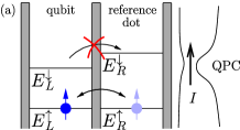
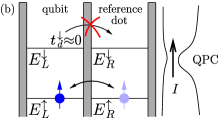
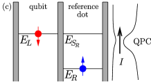
Figure 1: Electron spin read-out setup consisting of a double dot. The right “reference” dot is coupled capacitively to a QPC shown on the right. (a) Read out using different Zeeman splittings. For $\uparrow$, the electron tunnels between the two dots. For $\downarrow$, tunneling is suppressed by the detuning and the stationary state has a large contribution of the left dot since it has lower energy. This allows single-shot read out, i.e., $e=100\%$. (b) Spin-dependent tunneling amplitudes, $t_{\mathrm{d}}^{\downarrow}<t_{\mathrm{d}}^{\uparrow}$, also enable efficient read out. (c) Read out with the singlet state. Tunneling of spin $\uparrow$ to the reference dot is blocked due to the Pauli principle. (d) Schematic current vs. time during a single measurement. Here, $\tau_{\mathrm{dd}}$ is the time scale for tunneling and we assume $\Gamma_{\mathrm{tot}}>t_{\mathrm{d}}$, i.e., that the tunneling events can be resolved in the current.

Single spin read out. We now discuss several concrete read-out setups and their measurement efficiency. We consider a promising qubit, which is an electron spin confined in a quantum dot Loss97 ; reviewQdot . For the read out of such a spin qubit, the time scale is limited by the spin-flip time $T_{1}$, which has a lower bound of $\approx 100\>\mu\mathrm{s}$ FujisawaT1 ; HansonT1 (while $T_{2}$ is not of relevance here). One setup proposed in Ref. Loss97, is read out via a neighboring paramagnetic dot, where the qubit spin nucleates formation of a ferromagnetic domain. This leads to $p_{0}=p_{1}=\frac{3}{4}$ and thus $e=25\%$. Another idea is to transfer the qubit information from spin to charge Loss97 ; reviewQdot ; KaneSET ; Recher ; ELesr . For this, we propose to couple the qubit dot to a second (“reference”) dot footnoteRefLead and discuss several possibilities how that coupling can be made spin-dependent, see also Fig 1. The resulting charge distribution on the double dot will then depend on the qubit spin state and can be detected by coupling the double dot to an electrometer, such as a quantum point contact (QPC) Field ; Elzerman , see Fig 1 (or, alternatively, a single-electron transistor Rimberg ).

Read out with different Zeeman splittings. First, we propose a setup where efficiencies up to $100\,\%$ can be reached, see Fig. 1a. We take a double dot with different Zeeman splittings, $\Delta_{z}^{L,R}=E_{L,R}^{\downarrow}-E_{L,R}^{\uparrow}$, in each dot footnoteInhZeeman and consider a single electron on the double dot. For initial qubit state $\left.|\uparrow\rangle\right.$, the electron can tunnel from state $\left.|L_{\uparrow}\rangle\right.\widehat{=}$ ${}_{\!L}$${}_{\!R}$ to state $\left.|R_{\uparrow}\rangle\right.\widehat{=}$ ${}_{\!L}$${}_{\!R}$ and vice versa, and analogously for qubit state $\left.|\downarrow\rangle\right.$. We consider time scales shorter than $T_{1}$, thus the states with different spins are not coupled. Next, we define the detunings $\varepsilon_{\uparrow,\downarrow}=E_{L}^{\uparrow,\downarrow}-E_{R}^{\uparrow,\downarrow}$, which are different for the up and down states, $\varepsilon_{\downarrow}-\varepsilon_{\uparrow}=\Delta_{z}^{L}-\Delta_{z}^{R}\neq 0$. The stationary state of the double dot depends on $\varepsilon_{\uparrow,\downarrow}$ and so does the QPC current $\bar{I}_{\uparrow,\downarrow}$ [we show this below, see Eq. (5) and $\bar{I}_{\mathrm{incoh}}$]. Therefore, initial states $\left.|\uparrow\rangle\right.$ and $\left.|\downarrow\rangle\right.$ can be identified through distinguishable stationary currents fnUncertOutcome , $\bar{I}_{\uparrow}\neq\bar{I}_{\downarrow},$ thus $e={}$100% and single-shot read out is possible.

Spin-dependent tunneling provides another read-out scheme, see Fig. 1b, which we describe with spin-dependent tunneling amplitudes $t_{\mathrm{d}}^{\uparrow,\downarrow}$. For $t_{\mathrm{d}}^{\downarrow}\ll t_{\mathrm{d}}^{\uparrow}$, only spin $\uparrow$ tunnels onto the reference dot while tunneling of spin $\downarrow$ is suppressed. We assume the same Zeeman splitting in both dots and resonance $\varepsilon=0$. It turns out [Eq. (5)] that $\bar{I}_{\uparrow,\downarrow}$ depends on $t_{\mathrm{d}}^{\uparrow,\downarrow}$ and thus the state of the qubit can be measured. However, the decay to the stationary state is quite slow in case the qubit is $\left.|\downarrow\rangle\right.$, due to the suppressed tunneling amplitude $t_{\mathrm{d}}^{\downarrow}$ . Since the difference in charge distribution between qubit $\left.|\uparrow\rangle\right.$ and $\left.|\downarrow\rangle\right.$ is larger at short timescales, it can thus be advantageous to measure the time-dependent current (discussed toward the end).

Read out with Pauli principle. We now consider the case where the reference dot contains initially an electron in spin up ground state, see Fig. 1c. We assume gate voltages such that there are either two electrons on the right dot or one electron on each dot. Thus, we consider the 5 dimensional Hilbert space $\left.|{S_{R}}\rangle\right.\widehat{=}$ ${}_{\!L}$${}_{\!R}$, $\left.|\uparrow\downarrow\rangle\right.\widehat{=}$ ${}_{\!L}$${}_{\!R}$, $\left.|\downarrow\uparrow\rangle\right.\widehat{=}$ ${}_{\!L}$${}_{\!R}$, $\left.|T_{+}\rangle\right.\widehat{=}$ ${}_{\!L}$${}_{\!R}$, $\left.|T_{-}\rangle\right.\widehat{=}$ ${}_{\!L}$${}_{\!R}$. We define the “delocalized” singlet $\left.|S_{LR}\rangle\right.=(\left.|\uparrow\downarrow\rangle\right.-\left.|\downarrow\uparrow\rangle\right.)/\sqrt{2}$ and the triplet $\left.|T_{0}\rangle\right.=(\left.|\uparrow\downarrow\rangle\right.+\left.|\downarrow\uparrow\rangle\right.)/\sqrt{2}$. In the absence of tunneling, the corresponding energies are $E_{S_{R}}=2\epsilon_{R}+U$ and $E_{S_{LR}}=E_{T_{0,\pm}}=\epsilon_{L}+\epsilon_{R}$ with charging energy $U$ and single particle energies $\epsilon_{L,R}$. We can neglect states with two electrons on the qubit dot and the triplet states with two electrons on the reference dot, since they have a much larger energy (their admixture due to tunneling is small). We denote the state with an “extra” electron on the right dot as $\left.|R\rangle\right.\equiv\left.|S_{R}\rangle\right.$ with corresponding QPC current $I_{R}$. For state $\left.|L\rangle\right.\equiv\left.|S_{LR}\rangle\right.$ and for all triplet states, $\left.|T_{0,\pm}\rangle\right.$, the current is $I_{L}$. When tunneling is switched on and the qubit is initially in state $\left.|\uparrow\rangle\right.$, tunneling to the reference dot is blocked due to the Pauli exclusion principle OnoPauli . Thus, the double dot will remain in the (stationary) state $|T_{+}\rangle\langle T_{+}|$ and the current in the quantum dot remains $\langle I\rangle=I_{L}$ (a so-called non-demolition measurement). On the other hand, for an initial qubit state $\left.|\downarrow\rangle\right.$, the initial state of the double dot is $\left.|{\downarrow\uparrow}\rangle\right.=(\left.|T_{0}\rangle\right.-\left.|S_{LR}\rangle\right.)/\sqrt{2}$. The contribution $\left.|S_{LR}\rangle\right.$ of this superposition is tunnel coupled to $\left.|S_{R}\rangle\right.$ and will decay to the stationary state $\bar{\rho}$ with corresponding QPC current $\bar{I}$ (see below for an explicit evaluation). In contrast, the triplet contribution $\left.|T_{0}\rangle\right.$ is not tunnel-coupled to $\left.|S_{R}\rangle\right.$ due to spin conservation and does not decay. In total, the density matrix of the double dot decays into the stationary value $\frac{1}{2}(|T_{0}\rangle\langle T_{0}|+\bar{\rho})$. For $\varepsilon=0$, the ensemble-averaged QPC current for qubit $\left.|\downarrow\rangle\right.$ is $\langle I\rangle=\frac{1}{2}(I_{L}+\bar{I})\approx\frac{1}{4}(3I_{L}+I_{R})$ and can thus be distinguished from $I_{L}$ for qubit $\left.|\uparrow\rangle\right.$. However, in a single run of such a measurement, an initial qubit $\left.|\downarrow\rangle\right.$ decays either into $|T_{0}\rangle\langle T_{0}|$ or into $\bar{\rho}$, with 50% probability each. Since $|T_{0}\rangle\langle T_{0}|$ and $|T_{+}\rangle\langle T_{+}|$ lead to the same QPC current $I_{L}$, these two states are not distinguishable within this read-out scheme and single-shot read-out is not possible. The read out can now be described with the POVM model given above, with $\left.|\uparrow\rangle\right.\equiv\left.|0\rangle\right.$ and $\left.|\downarrow\rangle\right.\equiv\left.|1\rangle\right.$ and $A_{\uparrow}=I_{L}$; $A_{\downarrow}=\bar{I}$; $p_{\uparrow}=1$; and $p_{\downarrow}=\frac{1}{2}$. Thus, the measurement efficiency is $e={}$50%, i.e., to achieve a fidelity of $1-\alpha=99\%$, we need $n\geq 7$ read outs footnoteExpG .

An analogous read out is possible if the ground state of the reference dot is a triplet, say $\left.|RT_{+}\rangle\right.\widehat{=}$ ${}_{\!L}$${}_{\!R}$ which is lower than the other triplets ($\left.|RT_{0,-}\rangle\right.$, $\left.|RT_{-}\rangle\right.$) due to Zeeman splitting. Again, we assume that the reference dot is initially $\left.|\uparrow\rangle\right.$. First, for a qubit state $\left.|\uparrow\rangle\right.$ and at resonance, $\varepsilon=0$, tunneling into $\left.|RT_{+}\rangle\right.$ always occurs and $p_{\uparrow}=1$. Second, the qubit state $\left.|\downarrow\rangle\right.$ has an increased energy by the Zeeman splitting $\Delta_{z}$ and is thus at resonance with $\left.|RT_{0}\rangle\right.$ (which has also an increased energy). If the double dot is not projected onto the singlet (in $50\,\%$ of the cases), tunneling onto the reference dot will also occur, i.e., $p_{\downarrow}=\frac{1}{2}$. Thus, when one detects an additional charge on the reference dot, the initial state of the qubit is not known. We find again $e=50\%$.

Read-out model. So far we have introduced various spin read out schemes and the corresponding measurement efficiencies. In order to evaluate the signal strength $A_{0}-A_{1}$ for these schemes, we now calculate the stationary charge distribution $\bar{\rho}$ and QPC current $\bar{I}$ for the case when the electron can tunnel coherently between the two dots (as a function of the detuning and the tunnel coupling). We describe the read-out setup with the Hamiltonian $H=H_{\mathrm{d}}+V_{\mathrm{\mathrm{d}}}+H_{\mathrm{\mathrm{QPC}}}+V.$ Here, $H_{\mathrm{\mathrm{QPC}}}$ contains the energies of the (uncoupled) Fermi leads of the QPC. Further, $H_{\mathrm{d}}$ describes the double dot in the absence of tunneling, including orbital and electrostatic charging energies, $H_{\mathrm{d}}\left.|n\rangle\right.=E_{n}\left.|n\rangle\right.$. It thus contains $\varepsilon=E_{L}-E_{R}$, the detuning of the tunneling resonance. The inter-dot tunneling Hamiltonian is defined as $V_{\mathrm{\mathrm{d}}}=t_{\mathrm{d}}(\left.|R\rangle\right.\langle L|+\left.|L\rangle\right.\langle R|)$. (Note that for tunneling between $\left.|S_{LR}\rangle\right.$ and $\left.|S_{R}\rangle\right.$, $t_{\mathrm{d}}$ is $\sqrt{2}$ times the one-particle tunneling amplitude, since both states $\left.|{\uparrow\downarrow}\rangle\right.$ and $\left.|{\downarrow\uparrow}\rangle\right.$ are involved). $V$ is a tunneling Hamiltonian describing transport through the QPC. The tunneling amplitudes, $t^{\mathrm{Q}}_{L}$ and $t^{\mathrm{Q}}_{R}$, will be influenced by electrostatic effects, in particular by the charge distribution on the double dot. Thus, we model the measurement of the dot state via the QPC with $V=\left(t^{\mathrm{Q}}_{L}\left.|L\rangle\right.\langle L|+t^{\mathrm{Q}}_{R}\left.|R\rangle\right.\langle R|\right)\sum\big{(}c_{\mathrm{in}}^{\dagger}c_{\mathrm{out}}+\mathrm{h.c.}\big{)}$ Gurvitz ; Korotkov ; Goan . Here, $c_{\mathrm{in}}^{\dagger}$ and $c_{\mathrm{out}}^{\dagger}$ create electrons in the incoming and the outgoing leads of the QPC, where the sum is taken over all momentum and spin states. We derive the master equation for the reduced density matrix $\rho$ of the double dot. We use standard techniques and make a Born-Markov approximation in $V$ Blum ; footnoteTwoLevel . We allow for an arbitrary inter-dot tunnel coupling, i.e., we keep $V_{\mathrm{\mathrm{d}}}$ exactly, with energy splitting $E=\sqrt{4\,t_{\mathrm{d}}^{2}+\varepsilon^{2}}$ in the eigenbasis of $H_{\mathrm{d}}+V_{\mathrm{\mathrm{d}}}$. We obtain the master equation footnoteBloch

$${\dot{\rho}_{L}} = -{\dot{\rho}_{R}}=2t_{\mathrm{d}}\,\mathrm{Im}\,[{\rho_{RL}}],$$ (3)

$${\dot{\rho}_{RL}} = \left[it_{\mathrm{d}}+t_{\mathrm{d}}\frac{\Gamma_{\mathrm{Q}}\varepsilon}{E^{2}}(g_{\Sigma}-2g_{0})\right]\left({\rho_{R}}-{\rho_{L}}\right)$$ (4)

$$-\frac{t_{\mathrm{d}}\,{\Gamma_{\mathrm{Q}}}}{{\Delta\mu}}-\left(\kappa{\Gamma_{\mathrm{Q}}}+\Gamma_{\mathrm{i}}-i{\varepsilon}\right){\rho_{RL}},$$

for $\rho_{n}=\langle n|\rho\left.|n\rangle\right.$ and $\rho_{RL}=\langle R|\rho\left.|L\rangle\right.$. In comparison to previous work Gurvitz ; Korotkov ; Goan , we find an additional term, $-t_{\mathrm{d}}\,{\Gamma_{\mathrm{Q}}}/\Delta\mu$, which comes from treating $V_{\mathrm{\mathrm{d}}}$ exactly. We find that the current through the QPC is $I_{L}=2\pi\nu^{2}e\,\Delta\mu|t^{\mathrm{Q}}_{L}|^{2}$ for state $\left.|L\rangle\right.$ and analogously $I_{R}$ for state $\left.|R\rangle\right.$, and we choose $I_{L},\,I_{R}\geq 0$. Here, $\Delta\mu>0$ is the applied bias across the QPC and $\nu$ is the DOS at the Fermi energy of the leads connecting to the QPC. We define $g_{\pm}=g(\Delta\mu\pm E)$, $g_{\Sigma}=g_{+}+g_{-}$ and $g_{0}=g(\Delta\mu)$ with $g(x)=x\big{/}\Delta\mu\big{(}e^{x/kT}-1\big{)}$. The values $g_{\pm,\Sigma,0}$ vanish for $\Delta\mu\pm E>kT$. In this case, the decay rate due to the current assumes the known value Gurvitz ; Korotkov ; Goan , $\Gamma_{\mathrm{Q}}=\left(\sqrt{I_{L}}-\sqrt{I_{R}}\right)^{2}\big{/}\,2e$. Generally, the factor $\kappa=1+(4t_{\mathrm{d}}^{2}g_{\Sigma}+2\varepsilon^{2}g_{0})/E^{2}$ accounts for additional relaxation/dephasing due to particle hole excitations, induced, e.g., by thermal fluctuations of the QPC current. For almost equal currents, $I_{L,\,R}=I\,(1\pm\frac{1}{2}x)$, we have $\Gamma_{\mathrm{Q}}=Ix^{2}/8e+O(x^{4})$. Finally, by introducing the phenomenological rate $\Gamma_{\mathrm{i}}$ we have allowed for some intrinsic charge dephasing, which occurs on the time scale of nanoseconds FujisawaT2dd . For an initial state in the subspace $\{\left.|L\rangle\right.,\,\left.|R\rangle\right.\}$, we find the stationary solution of the double dot, $\bar{\rho}=\frac{1}{2}(1-\eta\varepsilon/\Delta\mu)\left.|L\rangle\right.\langle L|+\frac{1}{2}(1+\eta\varepsilon/\Delta\mu)\left.|R\rangle\right.\langle R|-\eta(t_{\mathrm{d}}/\Delta\mu)(\left.|R\rangle\right.\langle L|+\left.|L\rangle\right.\langle R|)$, where $\eta=\Gamma_{\mathrm{Q}}/[\Gamma_{\mathrm{Q}}(1+g_{\Sigma})+\Gamma_{\mathrm{i}}]$. Positivity of $\bar{\rho}$ is satisfied since $\eta\leq\Delta\mu/E$. The time decay to $\bar{\rho}$ is described by three rates, given as the roots of $P(\lambda)=\lambda^{3}+2\Gamma_{\mathrm{tot}}\lambda^{2}+\left(E^{2}+\Gamma_{\mathrm{tot}}^{2}\right)\lambda+4t_{\mathrm{d}}^{2}\big{[}\Gamma_{\mathrm{tot}}+\Gamma_{\mathrm{Q}}(g_{\Sigma}-2g_{0})\varepsilon^{2}/E^{2}\big{]}$, with $\Gamma_{\mathrm{tot}}=\kappa{\Gamma_{\mathrm{Q}}}+\Gamma_{\mathrm{i}}$. The stationary current through the QPC is given by $\bar{I}=\bar{\rho}_{L}I_{L}+\bar{\rho}_{R}I_{R}+2e\,t_{\mathrm{d}}\lambda(\Gamma_{\mathrm{Q}}/\Delta\mu)\,\mathrm{Re\,\bar{\rho}_{RL}}$ and thus becomes

$$\bar{I}=\frac{I_{L}+I_{R}}{2}+\eta\frac{\varepsilon}{2\Delta\mu}\left(I_{R}-I_{L}\right)-\eta\lambda\frac{2e\,\Gamma_{\mathrm{Q}}t_{\mathrm{d}}^{2}}{\Delta\mu^{2}},$$ (5)

where $\lambda=1-\Delta\mu(g_{-}-g_{+})/E$. We note that $\eta$ quantifies the effect of the detuning $\varepsilon$ on the QPC current. To reach maximal sensitivity, $\eta=1$, we need $I_{R}\lesssim I_{L}/10$ for $I\sim 1\,\mathrm{nA}$ and $\Gamma_{\mathrm{i}}\sim 10^{9}\>\mathrm{s}^{-1}$. In linear response, the current becomes $(I_{L}+I_{R})/2+\left(I_{R}-I_{L}\right)\varepsilon\tanh(E/2kT)[1-(\Gamma_{i}\Delta\mu/\Gamma_{\mathrm{Q}}E)\tanh(E/2kT)]/2E-2e\,t_{\mathrm{d}}^{2}\Gamma_{\mathrm{Q}}[1-E/kT$ $\sinh(E/kT)]/E^{2}+e\,t_{\mathrm{d}}^{2}\Gamma_{i}\Delta\mu[\sinh(E/kT)-E/kT][1-\Gamma_{i}\Delta\mu$ $\tanh(E/2kT)/\Gamma_{\mathrm{Q}}E]/E^{3}\cosh^{2}(E/kT)$. Note that the second term in Eq. (5) depends on $\varepsilon$, a property which can be used for read out, as we have discussed above. For example, for different Zeeman splittings and $\varepsilon_{\uparrow,\downarrow}=\pm\Delta\mu/2$, $\Gamma_{\mathrm{i}}=10^{9}\>\mathrm{s^{-1}}$, $I_{L}=1\,\mathrm{nA}$, and $I_{R}=0$, the current difference is $\bar{I}_{\downarrow}-\bar{I}_{\uparrow}=0.4\,\mathrm{nA}$, which reduces to $0.05\,\mathrm{nA}$ for $I_{R}=0.5\,\mathrm{nA}$. However, typical QPC currents currently reachable are $I_{L}=10\,\mathrm{nA}$ and $I_{R}=9.9\,\mathrm{nA}$, i.e., the relaxation of the double dot due to the QPC is suppressed, $\eta<10^{-3}$, and other relaxation channels become important.

Incoherent tunneling. So far, we have discussed coherent tunneling. We can also take incoherent tunneling into account, e.g., phonon assisted tunneling, by introducing relaxation rates in Eqs. (3),(4). For example, for detailed balance rates and neglecting coherent tunneling, we find the stationary current $\bar{I}_{\mathrm{incoh}}=\frac{1}{2}(I_{L}+I_{R})+\frac{1}{2}(I_{R}-I_{L})\tanh(\varepsilon/2kT)$ (which becomes $I_{R}$ for $\varepsilon>kT$). The QPC current again depends on $\varepsilon$ and can be used for spin read out. The current can also be measured on shorter time scales as we discuss now.

Read out with time-dependent currents is possible if there is sufficient time to distinguish $I_{L}$ from $I_{R}$ between two tunneling events to or from the reference dot, i.e., we consider $\Gamma_{\mathrm{tot}}>t_{\mathrm{d}}$. In this incoherent regime, the tunneling from qubit to reference dot occurs with a rate $W_{\uparrow}$ or $W_{\downarrow}$, depending on the qubit state, with, say, $W_{\downarrow}\ll W_{\uparrow}$. Such rates arise from spin-dependent tunneling, $t_{\mathrm{d}}^{\uparrow,\downarrow}$, or from different Zeeman splittings and tuning to tunneling resonance for, say, qubit $\left.|\uparrow\rangle\right.$ while qubit $\left.|\downarrow\rangle\right.$ is off-resonant, see Figs. 1a and 1b. For read out, the electron is initially on the left dot and the QPC current is $I_{L}$. Then, if the electron tunnels onto the reference dot within time $t$ and thus changes the QPC current to $I_{R}$, such a change would be interpreted as qubit in state $\left.|\uparrow\rangle\right.$, otherwise as qubit $\left.|\downarrow\rangle\right.$. For calculating the measurement efficiency $e$, we note that $p_{\uparrow}=p_{0}=1-e^{-tW_{\uparrow}}$ and $p_{\downarrow}=p_{1}=e^{-tW_{\downarrow}}$ (with this type of read out, $W_{\downarrow}$ corresponds to a loss of the information, i.e., describes “mixing” Schoen ). We then maximize $e$ by choosing a suitable $t$ and find efficiencies $e\gtrsim 50\,\%$ for $W_{\uparrow}/W_{\downarrow}\gtrsim 8.75$ and $e\gtrsim 90\,\%$ for $W_{\uparrow}/W_{\downarrow}\gtrsim 80$.

A more involved read out is to measure the current through the QPC at different times. The current as function of time switches between the values $I_{L}$ and $I_{R}$, i.e., shows telegraph noise, as sketched in Fig. 1d. Since the frequency of these switching events (roughly $W_{\uparrow}$ or $W_{\downarrow}$) depends on the spin, the QPC noise reveals the state of the qubit. Finally, at times of the order of the spin relaxation time $T_{1}$, the information about the qubit is lost. At each spin flip, the switching frequency changes ($W_{\uparrow}\leftrightarrow W_{\downarrow}$), which thus provides a way to measure $T_{1}$.

In conclusion, we have given the criterion when $n$-shot measurements are possible and have introduced the measurement efficiency $e$. For electron spin qubits, we have proposed several read-out schemes and have found efficiencies up to 100%, which allow single-shot read out. Other schemes, which are based on the Pauli principle, have a lower efficiency, $e=50\%$. We thank Ch. Leuenberger and F. Meier for discussions. We acknowledge support from the Swiss NSF, NCCR Nanoscience Basel, DARPA, and ARO.

References

• (1) M.A. Nielsen, I.L. Chuang, Quantum Computation and Quantum Information (Cambridge U. Press, New York, 2000).
• (2) D. Loss, D.P. DiVincenzo, Phys. Rev. A 57, 120 (1998).
• (3) L.M.K. Vandersypen et al. in Quantum Computing and Quantum Bits in Mesoscopic Systems, eds. A.J. Leggett et al. (Kluwer, NY, 2003), quant-ph/0207059.
• (4) A. Peres, Quantum Theory (Kluwer Academic, Amsterdam, 1993).
• (5) In other words, we assume a sufficient signal-to-noise ratio of the apparatus to distinguish the measurement outcome $A_{0}$ from $A_{1}$.
• (6) For a qubit in an arbitrary superposition $\alpha\left.|0\rangle\right.+\beta\left.|1\rangle\right.$, the expectation value of the measurement is $\langle\hat{A}\rangle=|\alpha|^{2}{\langle\hat{A}\rangle}_{0}+|\beta|^{2}{\langle\hat{A}\rangle}_{1}$, which allows to determine $|\alpha|^{2}$ and $|\beta|^{2}=1-|\alpha|^{2}$. (To measure the phase $\arg\alpha/\beta$, first some single qubit rotations need to be performed.) In order to differentiate a given $|\alpha|^{2}$ from a value $|\alpha^{\prime}|^{2}$, a sufficient $n$ is given by Eqs. (1) and (2) after replacing $p_{0}\to|\alpha|^{2}p_{0}+(1-|\alpha|^{2})(1-p_{1})$ and $p_{1}\to 1-|\alpha^{\prime}|^{2}p_{0}-(1-|\alpha^{\prime}|^{2})(1-p_{1})$.
• (7) K. Bosch, Grosses Lehrbuch der Statistik (R. Oldenbourg, Munich, 1996), pp. 379.
• (8) If $n$ is small, one can use Clopper-Pearson confidence intervals. However, if read out of one state is perfect, say $p_{0}=1$, we can no longer approximate with a normal distribution, even for large $n$. In that case, finding $A_{0}$ as outcome $n$ times in a row, even if the qubit is $\left.|1\rangle\right.$, i.e., read out fails, occurs with probability $(1-p_{1})^{n}$. Thus, $n\geq\log(\alpha)/\log(1-e)$ is sufficient for read out.
• (9) T. Fujisawa et al., Nature 419, 278 (2002).
• (10) R. Hanson et al., cond-mat/0303139.
• (11) B.E. Kane et al., Phys. Rev. B 61, 2961 (2000).
• (12) P. Recher, E.V. Sukhorukov, D. Loss, Phys. Rev. Lett. 85, 1962 (2000).
• (13) H.-A. Engel, D. Loss, Phys. Rev. Lett. 86, 4648 (2001); Phys. Rev. B 65, 195321 (2002).
• (14) Instead of a reference dot, the qubit dot can be coupled to a lead. To ensure that only electrons with, say, spin $\downarrow$ can tunnel, one can use spin-polarized leads or a Zeeman splitting on the dot and properly tuned energy levels ELesr .
• (15) M. Field et al., Phys. Rev. Lett. 70, 1311 (1993).
• (16) J. M. Elzerman et al., Phys. Rev. B 67, 161308 (2003).
• (17) W. Lu et al., Nature 423 (6938), 422 (2003).
• (18) This can be generated with (i) locally different magnetic fields. Or, with an inhomogeneous $g$ factor as follows. (ii) Spatial variation of dot location in a heterostructure, i.e., moving electrons up/down by gates etc. (iii) Similarly, produce a spatial variation with different orbital states by filling each dot with a different number of electrons. (iv) Different hyperfine interaction in each dot, say, by inducing a nuclear polarization in one dot by the QPC current. (v) Different Rashba interaction, (vi) optical Stark effect [C. Cohen-Tannoudji, J. Dupont-Roc, Phys. Rev. A 5, 968 (1972); J.A. Gupta et al., Science 292, 2458 (2001)], or (vii) differently distributed magnetic impurities in each dot.
• (19) K. Ono et al., Science 297, 1313 (2002).
• (20) S.A. Gurvitz, Phys. Rev. B 56, 15215 (1997).
• (21) A.N. Korotkov, Phys. Rev. B 63, 115403 (2001).
• (22) H.-S. Goan et al., Phys. Rev. B 63, 125326 (2001).
• (23) K. Blum, Density Matrix Theory and Applications (Plenum Press, New York, 1996), Chap.  8.
• (24) We map the two-level system $\{\left.|L\rangle\right.,\,\left.|R\rangle\right.\}$ onto a pseudo spin $\frac{1}{2}$ with Hamiltonian $H(t)=\frac{1}{2}\varepsilon\sigma_{z}+t_{\mathrm{d}}\sigma_{x}+X(t)\sigma_{z}+\frac{1}{2}(t^{\mathrm{Q}}_{L}+t^{\mathrm{Q}}_{R})V_{\mathrm{QPC}}(t)$. The fluctuations due to the QPC are $X(t)=\frac{1}{2}(t^{\mathrm{Q}}_{L}-t^{\mathrm{Q}}_{R})V_{\mathrm{QPC}}(t)$ with $V_{\mathrm{QPC}}(t)=e^{iH_{\mathrm{\mathrm{QPC}}}t}V_{\mathrm{QPC}}e^{-iH_{\mathrm{\mathrm{QPC}}}t}$.
• (25) We define ${\mathbf{P}}=\frac{1}{2}\mathrm{Tr}\,\rho\,\mbox{\boldmath{$\sigma$}}$ and write the master equation in the standard Bloch notation, $\dot{{\mathbf{P}}}=\mbox{\boldmath{$\omega$}}\times{\mathbf{P}}+\Gamma^{\prime}({\mathbf{P}}-{\mathbf{P}}_{0})$, with $\mbox{\boldmath{$\omega$}}=\left(2t_{\mathrm{d}},0,0\right)$ and $\Gamma^{\prime}{\mathbf{a}}=(0,\;-t_{\mathrm{d}}\Gamma_{\mathrm{Q}}/\Delta\mu-t_{\mathrm{d}}\Gamma_{\mathrm{Q}}(g_{\Sigma}-2g_{0})\varepsilon/E^{2},\;\varepsilon+t_{\mathrm{d}}\Gamma_{\mathrm{Q}}/\Delta\mu)\times{\mathbf{a}}+\Gamma{\mathbf{a}}$, where $\Gamma$ is symmetric with elements $\Gamma_{xy}=\Gamma_{yx}=-t_{\mathrm{d}}\Gamma_{\mathrm{Q}}/\Delta\mu$; $\Gamma_{xz}=\Gamma_{zx}=\Gamma_{xy}-t_{\mathrm{d}}\Gamma_{\mathrm{Q}}(g_{\Sigma}-2g_{0})\varepsilon/E^{2}$; $\Gamma_{yy}=-\Gamma_{\mathrm{Q}}(1+g_{\Sigma})+\Gamma_{\mathrm{Q}}(g_{\Sigma}-2g_{0})\varepsilon^{2}/E^{2}$; $\Gamma_{xx}=2\Gamma_{xy}+\Gamma_{yy}$; $\Gamma_{yz}=\Gamma_{zy}=\Gamma_{zz}=0$. Finally, $P_{0x}=P_{0y}=0$ and $P_{0z}=[t_{\mathrm{d}}\Gamma_{\mathrm{Q}}(2t_{\mathrm{d}}+\varepsilon)/(1+g_{\Sigma})\Delta\mu^{2}-\Gamma_{xy}]/\Gamma_{xz}$.
• (26) T. Hayashi et al., cond-mat/0308362.
• (27) Y. Makhlin, G. Schön, A. Shnirman, Phys. Rev. Lett. 85, 4578 (2000).