Discrete-time ratchets, the Fokker-Planck equation and Parrondo’s paradox

Abstract

Parrondo’s paradox; Fokker-Planck equation; Brownian ratchet. Parrondo’s games manifest the apparent paradox where losing strategies can be combined to win and have generated significant multidisciplinary interest in the literature. Here we review two recent approaches, based on the Fokker-Planck equation, that rigorously establish the connection between Parrondo’s games and a physical model known as the flashing Brownian ratchet. This gives rise to a new set of Parrondo’s games, of which the original games are a special case. For the first time, we perform a complete analysis of the new games via a discrete-time Markov chain (DTMC) analysis, producing winning rate equations and an exploration of the parameter space where the paradoxical behaviour occurs.

1 Introduction

In many physical and biological systems, combining processes may lead to counter-intuitive dynamics. For example, in control theory, the combination of two unstable systems can cause them to become stable (Allison & Abbott 2001a). In the theory of granular flow, drift can occur in a counter-intuitive direction (Rosato et al. 1987; Kestenbaum 1997). Also the switching between two transient diffusion processes in random media can form a positive recurrent process (Pinsky & Scheutzow 1992). Other interesting phenomena where physical processes drift in a counter-intuitive direction can be found (see for example Adjari & Prost 1993; Maslov & Zhang 1998; Westerhoff et al. 1986; Key 1987; Abbott 2001).

The Parrondo’s paradox (Harmer & Abbott 1999a,b; Harmer et al. 2000) is based on the combination of two negatively biased games – losing games – which when combined give rise to a positively biased game, that is, we obtain a winning game. This paradox is a translation of the physical model of the Brownian ratchet into game-theoretic terms. These games were first devised in 1996 by the Spanish physicist Juan M. R. Parrondo, who presented them in unpublished form in Torino, Italy (Parrondo 1996). They served as a pedagogical illustration of the flashing ratchet, where directed motion is obtained from the random or periodic alternation of two relaxation potentials acting on a Brownian particle, none of which individually produce any net flux (see Reimann 2002 for a complete review on ratchets).

These games have attracted much interest in other fields, for example quantum information theory (Abbott et al. 2002; Flitney et al. 2002; Meyer & Blumer 2002a; Lee et al. 2002a), control theory (Kocarev & Tasev 2002; Dinis & Parrondo 2002), Ising systems (Moraal 2000), pattern formation (Buceta et al. 2002a,b; Buceta & Lindenberg 2002), stochastic resonance (Allison & Abbott 2001b), random walks and diffusions (Cleuren & Van den Broeck 2002; Key et al. 2002; Kinderlehrer & Kowalczyk 2002; Percus & Percus 2002; Pyke 2002), economics (Boman et al. 2002), molecular motors in biology (Ait-Haddou & Herzog 2002; Heath et al. 2002) and biogenesis (Davies 2001). They have also been considered as quasi-birth-death processes (Latouche & Taylor 2003) and lattice gas automata (Meyer & Blumer 2002b).

Parrondo’s two original games are as follows. Game A is a simple tossing coin game, where a player increases (decreases) his capital in one unit if heads (tails) show up. The probability of winning is denoted by $p$ and the probability of losing is $1-p$.

Game B is a capital dependent game, where the probability of winning depends upon the actual capital of the player, modulo a given integer $M$. Therefore if the capital is $i$ the probability of winning $\pi_{i}$ is taken from the set $\{\pi_{0},\pi_{1},\dots,\pi_{M-1}\}$ as $\pi_{i}=\pi_{i\,{\rm mod}\,M}$. In the original version of game B, the number $M$ is set equal to three and the probability of winning can take only two values, $p_{1},\,p_{2}$, according to whether the capital of the player is a multiple of three or not, respectively. Using the previous notation we have $p_{1}\equiv\pi_{0}$, $p_{2}\equiv\pi_{1}=\pi_{2}$. The numerical values corresponding to the original Parrondo’s games (Harmer & Abbott 1999a) are:

$$\left\{\begin{array}[]{cc}p=&\frac{1}{2}-\epsilon,\\ p_{1}=&\frac{1}{10}-\epsilon,\\ p_{2}=&\frac{3}{4}-\epsilon,\end{array}\right.$$ (1)

where $\epsilon$ is a small biasing parameter introduced to control the three probabilities.

Although the original game B was based on a modulo rule, there are other versions of Parrondo’s games where this rule has been replaced by a history dependent rule (Parrondo et al. 2000); also combinations of two history dependent games are considered (Kay & Johnson 2002). Instead of a random alternation, also chaotic alternation between the games has been studied (Arena et al. 2003). Effects of cooperation between players have also been considered in Parrondo’s games, where the probabilities of game B depend on the actual state of the neighbours of the player (Toral 2001), also a redistribution of capital between the players has been considered (Toral 2002). Other variations of collective games have recently appeared (Mihailović & Rajković 2003a,b). For a full review of Parrondo’s paradox see Harmer & Abbott 2002.

Games A and B appearing in the Parrondo’s paradox can be thought of as diffusion processes under the action of a external potential. However, they do not have the more general form of a natural diffusion proces, because the capital will always change with every game played, whereas in the most general diffusion process a particle can either move up or down or remain in the same position at a given time. In this article we present a new version of Parrondo’s games, where a new transition probability is taken into account. We introduce a self-transition probability, that is, the capital of the player now can remain the same after a game played with a probability $\rho_{i}$, taken from the set $\{\rho_{0},\rho_{1},\dots,\rho_{M-1}\}$ as $\rho_{i}=\rho_{i\,{\rm mod}\,M}$. Again, for simplicity, we will only consider the case of $M=3$ with just two possible self-transition probabilities, $r_{1},\,r_{2}$, depending only on the capital being a multiple of three or not: $r_{1}\equiv\rho_{0},\,r_{2}\equiv\rho_{1}=\rho_{2}$.

As we will show, the significance of this new version is a natural evolution of Parrondo’s games, which can now be rigorously derived from the Fokker-Planck equation, based on a physical flashing ratchet model.

The outline of this paper is as follows. In section $2$ we briefly review two relations concerning Parrondo’s games and the Fokker-Planck equation. In both relations it is straightforward the inclusion of self-probabilities. In Sec. $3$ we give a mathematical analysis of the new games using discrete-time Markov chains and derive conditions for the paradox to appear. In Sec. $4$ we calculate the rates of winning, describe the parameter space and present numerical simulations which confirm and extend the theoretical analysis. Finally, in section $5$ we provide a brief discussion of the results.

2 The Flashing ratchet and the Fokker-Planck equation

Despite the fact that Parrondo’s paradox was inspired by the flashing ratchet, the relation between both has only been made quantitative recently, when two different approaches have established a formal relation between Parrondo’s games and the physical model of the flashing ratchet (Allison & Abbott 2002 and Toral et al. 2003a). We now very briefly review both approaches.

In the scheme proposed by Allison & Abbott (2002), the starting point is the following general Fokker–Planck equation (see Horsthemke and Lefever, 1984), for the probability $P(x,t)$ of a Brownian particle moving in a time-dependent one-dimensional potential $V(x,t)$:

$$D\frac{\partial^{2}P}{\partial x^{2}}-P\frac{\partial\alpha}{\partial x}-\alpha\frac{\partial P}{\partial x}-\frac{\partial P}{\partial t}=0,$$ (2)

where $\alpha$ and $D$ are referred to as the infinitesimal first and second moments of diffusion, respectively; $D$ has a constant value – “Fick’s law constant”– while $\alpha(x,t)$ is a function related to the applied potential $V(x,t)$ by the equation

$$\alpha(x,t)=-u\frac{\partial}{\partial x}V(x,t),$$ (3)

where $u$ denotes the mobility of the Brownian particle.

Then (2) is discretized using a finite difference approximation obtaining

$$P_{i,j}=a_{-1}^{i,j}\cdot P_{i-1,j-1}+a_{0}^{i,j}\cdot P_{i,j-1}+a_{+1}^{i,j}\cdot P_{i+1,j-1}$$ (4)

where

$$a_{-1}^{i,j}=\frac{\frac{D\tau}{\lambda^{2}}+\frac{\alpha(i,j)\tau}{2\lambda}}{\frac{\alpha(i+1,j-1)-\alpha(i-1,j-1)}{2\lambda}\tau+1}$$ (5)

$$a_{0}^{i,j}=\frac{-2\frac{D\tau}{\lambda^{2}}+1}{\frac{\alpha(i+1,j-1)-\alpha(i-1,j-1)}{2\lambda}\tau+1}$$ (6)

$$a_{+1}^{i,j}=\frac{\frac{D\tau}{\lambda^{2}}-\frac{\alpha(i,j)\tau}{2\lambda}}{\frac{\alpha(i+1,j-1)-\alpha(i-1,j-1)}{2\lambda}\tau+1}\,.$$ (7)

Here the index $i$ denotes the discretized space $x=i\lambda$, whereas $j$ denotes the discretized time $t=j\tau$ ; $\lambda$ and $\tau$ account for the space and time discretization steps respectively.

This discretized form (4) of the Fokker–Planck equation is compared to the master equation for any of the gambling games used in Parrondo’s paradox

$$P_{i,j}=\pi_{i-1}\cdot P_{i-1,j-1}+\rho_{i}\cdot P_{i,j-1}+(1-\pi_{i+1}-\rho_{i+1})\cdot P_{i+1,j-1}$$ (8)

where $P_{i,j}$ denotes the probability that the player has a capital $i$ at the $j$ play. In the original Parrondo games the self-transition probability is zero, so that the term $\rho_{i}$ is set to zero in the following calculations.

Combining (4) and (8) we get

$$\frac{\pi_{i-1}}{1-\pi_{i+1}}=\frac{a_{-1}^{i,j}}{a_{+1}^{i,j}}=\frac{1+\frac{\lambda}{2D\tau}\alpha(i,j)}{1-\frac{\lambda}{2D\tau}\alpha(i,j)}$$ (9)

and it follows that the function $\alpha(i,j)\equiv\alpha_{i}$ is independent of the time index $j$:

$$\alpha_{i}=\frac{2D}{\lambda}\,\frac{\pi_{i-1}-(1-\pi_{i+1})}{\pi_{i-1}+(1-\pi_{i+1})}\,.$$ (10)

Finally, the discretized values of the potential are obtained combining (3) with (10),

$$V_{i}=-\frac{2D}{u}\sum^{i}_{k=0}\frac{1-\left(\frac{1-\pi_{k+1}}{\pi_{k-1}}\right)}{1+\left(\frac{1-\pi_{k+1}}{\pi_{k-1}}\right)}.$$ (11)

This equation allows one to obtain the discretized version of the physical potential $V_{i}$ in terms of the probabilities $\pi_{i}$ of the games.

A second relation between the Fokker–Planck equation and the master equation has been proposed by Toral et al. (2003a). Unlike the first approach described above now the starting point is not the Fokker–Planck equation but rather the rewriting of the master equation (8) in the form of a continuity equation for the probability:

$$P_{i,j}-P_{i,j-1}=-\left[J_{i+1,j}-J_{i,j}\right]$$ (12)

where the current $J_{i,j}$ is given by:

$$J_{i,j}=\frac{1}{2}\left[F_{i}P_{i,j}+F_{i-1}P_{i-1,j}\right]-\left[D_{i}P_{i,j}-D_{i-1}P_{i-1,j}\right]$$ (13)

and

$$F_{i}=2\pi_{i}+\rho_{i}-1,\hskip 56.9055ptD_{i}=\frac{1-\rho_{i}}{2}\,.$$ (14)

These coefficients can be related with their analogous terms corresponding to a discretization of the Fokker–Planck equation for a probability $P(x,t)$

$$\frac{\partial P(x,t)}{\partial t}=-\frac{\partial J(x,t)}{\partial x}$$ (15)

with a current

$$J(x,t)=F(x)P(x,t)-\frac{\partial[D(x)P(x,t)]}{\partial x}$$ (16)

for a general drift $F(x)$ and diffusion $D(x)$.

Considering again the case $\rho_{i}=0$, we have

$$D_{i}\equiv D=1/2\hskip 56.9055ptF_{i}=-1+2\pi_{i}$$ (17)

and the following form for the current:

$$J_{i,j}=\pi_{i-1}P_{i-1,j}-(1-\pi_{i})P_{i,j}$$ (18)

which is nothing but the probability flux from state $i-1$ to state $i$.

The relation between the external potential $V_{i}$ and the games probabilities is in this formulation written as:

$$V_{i}=-\frac{1}{2}\sum_{k=1}^{i}\ln\left[\frac{1+F_{k-1}}{1-F_{k}}\right]=-\frac{1}{2}\sum_{k=1}^{i}\ln\left[\frac{\pi_{k-1}}{1-\pi_{k}}\right]$$ (19)

where the value $V_{0}=0$ has been adopted for convenience. This equation is the main result concerning the relation between the games probabilities $\pi_{i}$ and the discretized version of the potential $V_{i}$. As with (11), through (19) we can obtain the potential that corresponds to a Parrondo game. Notice that both approaches yield different values for the potential $V_{i}$ corresponding to a set of games probabilities $\{\pi_{0},\dots,\pi_{M-1}\}$. For instance, in the case of a fair game, the potential given by (19) is a periodic function $V_{i+M}=V_{i}$, (Toral et al. 2003b). Nevertheless, it can be shown that both potentials coincide in the limit of an infinitessimaly small space discretized step $\lambda$.

It is possible to solve the master equation (12) using a constant current $J_{i,j}=J$, together with the boundary condition $P_{i}^{st}=P_{i+M}^{st}$ in order to obtain the stationary probability distribution $P_{i}^{st}$. The result is:

$$P_{i}^{st}=N{\rm e}^{-2V_{i}}\left[1-\frac{2J}{N}\sum_{j=1}^{i}\frac{{\rm e}^{2V_{j}}}{1-F_{j}}\right]$$ (20)

with a current

$$J=N\frac{{\rm e}^{-2V_{M}}-1}{2\sum_{j=1}^{M}\frac{{\rm e}^{2V_{j}}}{1-F_{j}}}$$ (21)

and $N$ is a normalization constant obtained from $\sum_{k=0}^{M-1}P_{k}^{st}=1$.

The inverse problem of obtaining the game probabilities in terms of the potential can also be done. It requires solving (19) with the boundary condition $F_{0}=F_{M}$. The solution is given by

$$F_{i}=(-1)^{i}{\rm e}^{2V_{i}}\left[\frac{\sum_{j=1}^{M}(-1)^{j}[{\rm e}^{-2V_{j}}-{\rm e}^{-2V_{j-1}}]}{(-1)^{M}{\rm e}^{2(V_{0}-V_{M})}-1}+\sum_{j=1}^{i}(-1)^{j}[{\rm e}^{-2V_{j}}-{\rm e}^{-2V_{j-1}}]\right]$$ (22)

which, via $\pi_{i}=(1+F_{i})/2$, allows one to obtain the probabilities $\pi_{i}$ in terms of the potential $V_{i}$. It is clear that the additional condition $\pi_{i}\in[0,1],\,\forall i$ must be fulfilled by any acceptable solution.

To sum up, we have two approaches, either (11) or (19), that allow one to obtain the potential corresponding to a set of probabilities $(\pi_{0},\dots,\pi_{M-1})$ defining a Parrondo game. In both approaches it is very easy to introduce self-probabilities $\rho_{i}\neq 0$. Therefore, we find it interesting to investigate the effect of these terms in the Parrondo’s paradox. Therefore we introduce a new branch in the original games (Harmer & Abbott 2002) that accounts for the self-transition probability denoted by $r_{i}$. The new diagrams for the games A and B are presented in figure 1. In the next section we will investigate the effect of this new inclusion upon the Parrondo effect.

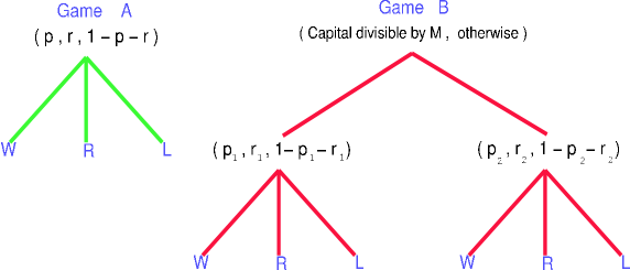
Figure 1: Probability trees of the new games A and B. Game A is formed by three branches, denoting the three possibilities of winning (W), remaining in the same state (R) and losing (L). Note that game B has a capital dependent rule and therefore is not a martingale.

3 Analysis of the new Parrondo games with self-transitions

3.1 Game A

We start with the new game A, where the probability of winning is $p$, the probability of remaining with the same capital will be denoted as $r$, and we lose with probability $q=1-r-p$ .

Following the same reasoning as Harmer et al. (2000) we will calculate the probability $f_{j}$ that our capital reaches zero in a finite number of plays, supposing that initially we have a given capital of $j$ units. From Markov chain analysis (Karlin 1973) we have that

• $f_{j}=1$ for all $j\geq{0}$, and so the game is either fair or losing; or

• $f_{j}<1$ for all $j>0$, in which case the game can be winning because there is a certain probability that our capital can grow indefinitely.

We are looking for the set of numbers $\{f_{j}\}$ that correspond to the minimal non-negative solution of the equation

$$f_{j}=p\cdot f_{j+1}+r\cdot f_{j}+q\cdot f_{j-1}\,,\hskip 14.22636ptj\geq 1$$ (23)

with the boundary condition

$$f_{0}=1\,.$$ (24)

With a subtle rearrangement, (23) can be put in the following form

$$f_{j}=\frac{p}{1-r}\cdot f_{j+1}+\frac{q}{1-r}\cdot f_{j-1}\,.$$ (25)

Whose solution, for the initial condition (24), is $f_{j}=A\cdot[(\frac{1-p-r}{p})^{j}-1]+1$, where $A$ is a constant. For the minimal non-negative solution we obtain

$$f_{j}=\min\left[1,\left(\frac{1-p-r}{p}\right)^{j}\right].$$ (26)

So we can see that the new game A is a winning game for

$$\frac{1-p-r}{p}<1,$$ (27)

is a losing game for

$$\frac{1-p-r}{p}>1,$$ (28)

and is a fair game for

$$\frac{1-p-r}{p}=1.$$ (29)

3.2 Game B

We now analyze the new game B. Like game A, we have introduced the probabilities of a self-transition in each state, that is, if the capital is a multiple of three we have a probability $r_{1}$ of remaining in the same state, whereas if the capital is not a multiple of three then the probability is $r_{2}$. The rest of the probabilities will follow the same notation as in the original game B, so we have the following scheme

$$\left\{\begin{array}[]{cc}\mathrm{mod(capital,3)}=0\rightarrow p_{1},r_{1},q_{1}\\ \\ \mathrm{mod(capital,3)}\neq 0\rightarrow p_{2},r_{2},q_{2}.\end{array}\right.$$ (30)

As in the case of game A, we will follow similar reasoning as Harmer et al. (2000) but for game B. Let $g_{j}$ be the probability that the capital will reach the zeroth state in a finite number of plays, supposing an initial capital of $j$ units. Again, from Markov chain theory we have

• $g_{j}=1$ for all $j\geq{0}$, so game B is either fair or losing; or

• $g_{j}<1$ for all $j>0$, in which case game B can be winning because there is a certain probability for the capital to grow indefinitely.

For $j\geq{1}$, the following set of recurrence equations must be solved:

$$\begin{array}[]{rcll}g_{3j}&=&p_{1}\cdot g_{3j+1}+r_{1}\cdot g_{3j}+(1-p_{1}-r_{1})\cdot g_{3j-1},&\hskip 11.38092ptj\geq 1\\ g_{3j+1}&=&p_{2}\cdot g_{3j+2}+r_{2}\cdot g_{3j+1}+(1-p_{2}-r_{2})\cdot g_{3j},&\hskip 11.38092ptj\geq 0\\ g_{3j+2}&=&p_{2}\cdot g_{3j+3}+r_{2}\cdot g_{3j+2}+(1-p_{2}-r_{2})\cdot g_{3j+1},&\hskip 11.38092ptj\geq 0\,.\end{array}$$ (31)

As in game A, we are looking for the set of numbers $\{g_{j}\}$ that correspond to the minimal non-negative solution. Eliminating terms $g_{3j-1}$, $g_{3j+1}$ and $g_{3j+2}$ from (31) we get

$$[p_{1}p^{2}_{2}+(1-p_{1}-r_{1})(1-p_{2}-r_{2})^{2}]\cdot g_{3j}=p_{1}p^{2}_{2}\cdot g_{3j+3}+(1-p_{1}-r_{1})(1-p_{2}-r_{2})^{2}\cdot g_{3j-3}\,.$$ (32)

Considering the same boundary condition as in game A, $g_{0}=1$, the last equation has a general solution of the form $g_{3j}=B\cdot\left[\left(\frac{(1-p_{1}-r_{1})(1-p_{2}-r_{2})^{2}}{p_{1}p^{2}_{2}}\right)^{j}-1\right]+1$, where $B$ is a constant. For the minimal non-negative solution we obtain

$$g_{3j}=\min\left[1,\left(\frac{(1-p_{1}-r_{1})(1-p_{2}-r_{2})^{2}}{p_{1}p^{2}_{2}}\right)^{j}\right].$$ (33)

It can be verified that the same solution (33) will be obtained solving (31) for $g_{3j+1}$ and $g_{3j+2}$, leading all them to the same condition for the probabilities of the games.

As with game A, game B will be winning if

$$\frac{(1-p_{1}-r_{1})(1-p_{2}-r_{2})^{2}}{p_{1}p^{2}_{2}}<1,$$ (34)

losing if

$$\frac{(1-p_{1}-r_{1})(1-p_{2}-r_{2})^{2}}{p_{1}p^{2}_{2}}>1,$$ (35)

and fair if

$$\frac{(1-p_{1}-r_{1})(1-p_{2}-r_{2})^{2}}{p_{1}p^{2}_{2}}=1.$$ (36)

3.3 Game AB

Now we will turn to the random alternation of games A and B with probability $\gamma$. This will be named as game AB. For this game AB we have the following (primed) probabilities

• if the capital is a multiple of three

  $$\left\{\begin{array}[]{cc}p^{\prime}_{1}=\gamma\cdot p+(1-\gamma)\cdot p_{1},\\ r^{\prime}_{1}=\gamma\cdot r+(1-\gamma)\cdot r_{1},\\ \end{array}\right.$$ (37)

• if the capital is not multiple of three

  $$\left\{\begin{array}[]{cc}p^{\prime}_{2}=\gamma\cdot p+(1-\gamma)\cdot p_{2},\\ r^{\prime}_{2}=\gamma\cdot r+(1-\gamma)\cdot r_{2}.\\ \end{array}\right.$$ (38)

The same reasoning as with game B can be made but with the new probabilities $p^{\prime}_{1}$, $r^{\prime}_{1}$, $p^{\prime}_{2}$, $r^{\prime}_{2}$ instead of $p_{1}$, $r_{1}$, $p_{2}$, $r_{2}$. Eventually we obtain that game AB will be winning if

$$\frac{(1-p^{\prime}_{1}-r^{\prime}_{1})(1-p^{\prime}_{2}-r^{\prime}_{2})^{2}}{p^{\prime}_{1}p^{\prime 2}_{2}}<1,$$ (39)

losing if

$$\frac{(1-p^{\prime}_{1}-r^{\prime}_{1})(1-p^{\prime}_{2}-r^{\prime}_{2})^{2}}{p^{\prime}_{1}p^{\prime 2}_{2}}>1,$$ (40)

and fair if

$$\frac{(1-p^{\prime}_{1}-r^{\prime}_{1})(1-p^{\prime}_{2}-r^{\prime}_{2})^{2}}{p^{\prime}_{1}p^{\prime 2}_{2}}=1.$$ (41)

The paradox will be present if games A and B are losing, while game AB is winning. In this framework this means that the conditions (28), (35) and (39) must be satisfied simultaneously. In order to obtain sets of probabilities fulfilling theses conditions we have first obtained sets of probabilities yielding fair A and B games but such that AB is a winning game, and then introducing a small biasing parameter $\epsilon$ making game A and game B losing games, but still keeping a winning AB game. As an example, we give some sets of probabilities that fulfill these conditions:

$$\begin{array}[]{rlllllll}(a)&p&=\frac{9}{20}-\epsilon,{}&r=\frac{1}{10},{}&p_{1}=\frac{9}{100}-\epsilon,{}&r_{1}=\frac{1}{10},{}&p_{2}=\frac{3}{5}-\epsilon,{}&r_{2}=\frac{1}{5},\cr(b)&p&=\frac{9}{20}-\epsilon,{}&r=\frac{1}{10},{}&p_{1}=\frac{509}{5000}-\epsilon,&r_{1}=\frac{1}{10},&p_{2}=\frac{7}{10}-\epsilon,{}&r_{2}=\frac{1}{20},\cr(c)&p&=\frac{9}{20}-\epsilon,{}&r=\frac{1}{10},{}&p_{1}=\frac{3}{25}-\epsilon,{}&r_{1}=\frac{2}{5},{}&p_{2}=\frac{3}{5}-\epsilon,{}&r_{2}=\frac{1}{10},\cr(d)&p&=\frac{1}{4}-\epsilon,{}&r=\frac{1}{2},{}&p_{1}=\frac{3}{25}-\epsilon,{}&r_{1}=\frac{2}{5},{}&p_{2}=\frac{3}{5}-\epsilon,{}&r_{2}=\frac{1}{10}.\end{array}$$ (42)

4 Properties of the Games

4.1 Rate of winning

If we consider the capital of a player at play number $n$, $X_{n}$ modulo $M$, we can perform a Discrete Time Markov Chain (DTMC) analysis of the games with a state-space $\{0,1,\ldots,M-1\}$ (c.f. Harmer et al. 2001). For the case of Parrondo’s games we have $M=3$, so the following set of difference equations for the probability distribution can be obtained (Lee et al. 2002b):

$$\begin{array}[]{cc}P_{0,n+1}&=p_{2}\cdot P_{2,n}+r_{1}\cdot P_{0,n}+q_{2}\cdot P_{1,n}\\ P_{1,n+1}&=p_{1}\cdot P_{0,n}+r_{2}\cdot P_{1,n}+q_{2}\cdot P_{2,n}\\ P_{2,n+1}&=p_{2}\cdot P_{1,n}+r_{2}\cdot P_{2,n}+q_{1}\cdot P_{0,n}\\ \end{array}$$ (43)

which can be put in a matrix form as $\textbf{P}_{n+1}=\mathbb{T}\cdot\textbf{P}_{n}$, where

$$\mathbb{T}=\left(\begin{array}[]{ccc}r_{1}&q_{2}&p_{2}\\ p_{1}&r_{2}&q_{2}\\ q_{1}&p_{2}&r_{2}\\ \end{array}\right)$$ (44)

and

$$\textbf{P}_{n}=\left(\begin{array}[]{c}P_{0,n}\\ P_{1,n}\\ P_{2,n}\\ \end{array}\right).$$ (45)

In the limiting case where $n\rightarrow\infty$ the system will tend to a stationary state characterized by

$$\mathbf{\Pi}=\mathbb{T}\cdot\mathbf{\Pi}$$ (46)

where $\lim_{n\rightarrow\infty}\mathbf{P}_{n}=\mathbf{\Pi}$.

Solving (46) is equivalent to solving an eigenvalue problem. As we are dealing with Markov chains, we know that there will be an eigenvalue $\lambda=1$ and the rest will be under $1$ (Karlin 1973). For the $\lambda=1$ value we obtain the following eigenvector giving the stationary probability distribution in terms of the games’ probabilities.

$$\mathbf{\Pi}\equiv\left(\begin{array}[]{c}\Pi_{0}\\ \Pi_{1}\\ \Pi_{2}\end{array}\right)=\frac{1}{D}\left(\begin{array}[]{c}(1-r_{2})^{2}-p_{2}\cdot(1-p_{2}-r_{2})\\ (1-r_{1})(1-r_{2})-p_{2}\cdot(1-p_{1}-r_{1})\\ (1-r_{1})(1-r_{2})-p_{1}\cdot(1-p_{2}-r_{2})\\ \end{array}\right)$$ (47)

where $D$ is a normalization constant given by

$$D=(1-r_{2})^{2}+2(1-r_{1})(1-r_{2})-p_{2}(2-p_{2}-r_{2}-r_{1}-p_{1})-p_{1}(1-p_{2}-r_{2}).$$ (48)

The rate of winning at the $n$–th step, has the general expression (Harmer et al. 2001)

$$r(n)\equiv E[X_{n+1}]-E[X_{n}]=\sum^{\infty}_{i=-\infty}{i\cdot[P_{i,n+1}-P_{i,n}]}\,.$$ (49)

Using these expressions and by similar techniques to those employed in Harmer et al. (2001) it is possible to obtain the stationary rate of winning for the new games introduced in the previous section. The results are, for game A:

$$r^{st}_{A}=2p+r-1$$ (50)

and for game B

$$r^{st}_{B} = 2p_{2}+r_{2}-1+[q_{2}-p_{2}+p_{1}-q_{1}]\cdot\Pi_{0}$$ (51)

$$= \frac{3}{D}\,(p_{1}p^{2}_{2}-(1-p_{1}-r_{1})(1-p_{2}-r_{2})^{2})$$

where $D$ is given by (48).

It is an easy task to check that when $r_{1}=r_{2}=0$ we recover the known expressions for the original games obtained by Harmer et al. (2001). To obtain the stationary rate for the randomized game AB we just need to replace in the above expression the probabilities from (37) and (38).

Within this context the paradox appears when $r^{st}_{A}\leq 0$, $r^{st}_{B}\leq 0$ and $r^{st}_{AB}>0$. If, for example, we use the values from (42d) and a switching probability $\gamma=1/2$, we obtain the following stationary rates for game A, game B and the random combination AB:

$$r^{st}_{A} = -2\epsilon,$$

$$r^{st}_{B} = \frac{-\epsilon\,(441-120\epsilon+1000\epsilon^{2})}{231-40\epsilon+500\epsilon^{2}},$$ (52)

$$r^{st}_{AB} = \frac{93-9828\epsilon+1920\epsilon^{2}-32000\epsilon^{3}}{2\,(2499-320\epsilon+8000\epsilon^{2})}\,.$$

which yield the desired paradoxical result for small $\epsilon>0$.

We can also evaluate the stationary rate of winning when both the probability of winning and the self-transition probability for the games vary with a parameter $\epsilon$ as $p=p-\frac{\epsilon}{2}$ and $r=r+\epsilon$, so that normalization is preserved. Using the set of probabilities derived from (42d), namely $p=\frac{1}{4}-\frac{\epsilon}{2}\,,r=\frac{1}{2}+\epsilon\,,p_{1}=\frac{3}{25}-\frac{\epsilon}{2}\,,r_{1}={\frac{2}{5}}+\epsilon\,,p_{2}=\frac{3}{5}-\frac{\epsilon}{2}\,,r_{2}=\frac{1}{10}+\epsilon$, the result is:

$$r^{st}_{A} = 0,$$

$$r^{st}_{B} = \frac{-\epsilon\,(21-20\epsilon)}{2\,(77-200\epsilon+125\epsilon^{2})},$$ (53)

$$r^{st}_{AB} = \frac{31-164\epsilon+160\epsilon^{2}}{2\,(833-2600\epsilon+2000\epsilon^{2})}\,,$$

again a paradoxical result.

A comparison between the expressions for the rates of winning of the original Parrondo games (Harmer et al. 2001) and the new games can be done in two ways. The first one consists in comparing two games with the same probabilities of winning, say original game A with probabilities $p=\frac{1}{2}$ and $q=\frac{1}{2}$ and the new game A with probabilities $p_{\mathrm{new}}=\frac{1}{2}$, $r_{\mathrm{new}}=\frac{1}{4}$ and $q_{\mathrm{new}}=\frac{1}{4}$. In this case we can think of the ‘old’ probability of losing $q$ as taking the place of the self-transition probability $r_{\mathrm{new}}$ and the new probability of losing $q_{\mathrm{new}}$. In this way we obtain a higher rate of winning in the new game A than in the original game – remember that the new game A has an extra term $r$ in the rate of winning compared to the original rate, and this extra term is what gives rise to the higher value. The same reasoning applies for game B, leading to the same conclusion.

The other possibility could be to compare the two games with the same probability of losing. In this case, we follow the same reasoning as before, but now we can imagine the ‘old’ probability of winning as replacing the winning and self-transition probabilities of the new game. What we now obtain is a lower rate of winning for the new game compared to the original one. An easy way of checking this is by rewriting (50) and (51) as

$$r^{st}_{A}=p-q$$ (54)

$$r^{st}_{B}=\frac{3}{D}\,(p_{1}p^{2}_{2}-q_{1}q_{2}^{2}).$$

So for the same value of $q$ but a lower value of $p$ we obtain a lower value for the rates of game A and B.

Figure 2: Parameter space corresponding to the values $r=\frac{1}{4}$, $r_{1}=\frac{1}{8}$ and $r_{2}=\frac{1}{10}$. The actual region where the paradox exists is delimited by the plane $p_{1}=0$ and the triangular region situated at the frontal face, where all the planes intersect.

We now explore the range of probabilities in which the Parrondo effect takes place. We restrict ourselves to the case $M=3$ and $\gamma=1/2$ used in the previous formulae.

The fact that we have introduced three new probabilities complicates the representation of the parameter space as we have six variables altogether, two variables $\{p,r\}$ from game A and four variables $\{p_{1},r_{1},p_{2},r_{2}\}$ coming from game B. In order to simplify this high number of variables, some probabilities must be set so that a representation in three dimensions will be possible. In our case we will fix the variables $\{r,r_{1},r_{2}\}$ so that the surfaces can be represented in the parameter space $\{p,p_{1},p_{2}\}$.

In figure 2 we can see the resulting region where the paradox exists for the variables $r=\frac{1}{4}$, $r_{1}=\frac{1}{8}$ and $r_{2}=\frac{1}{10}$. Some animations have shown that the volume where the paradox takes place, gradually shrinks to zero as the variables $r$, $r_{1}$ and $r_{2}$ increase from zero to their maximum value of one.

Another interesting fact that we have encountered, which remains an open question, is the impossibility of obtaining the equivalent parameter space to figure 2 with the fixed variables ${p,p_{1},p_{2}}$ and with the parameter space variables ${r,r_{1},r_{2}}$ instead – it is possible to obtain the planes for games A and B, but not for the randomized game AB.

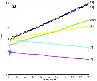
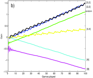
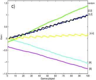
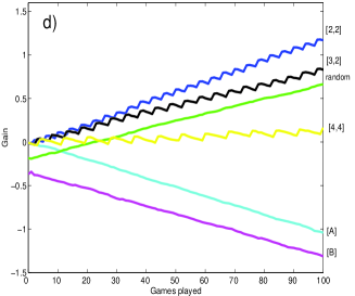
Figure 3: Average gain as a function of the number of games played coming from numerical simulation of Parrondo’s games with differet sets of probabilities. The notation $[a,b]$ indicates that game A was played $a$ times and game B $b$ times. The gains were averaged over 50 000 realizations of the games. a) Simulation corresponding to the probabilities (42a) and $\epsilon=\frac{1}{500}$; b) probabilities (42b) and $\epsilon=\frac{1}{200}$; c) probabilities (42c) and $\epsilon=\frac{1}{200}$; d) probabilities (42d) and $\epsilon=\frac{1}{200}$ .

4.2 Simulations and discussion

We have analyzed the new games A and B, and obtained the conditions in order to reproduce the Parrondo effect. We now present some simulations to verify that the paradox is present for a different range of probabilities – see figure 3. Some interesting features can be observed from these graphs. First it can be noticed that the performance of random or deterministic alternation of the games drastically changes with the parameters.

We use the notation $[a,b]$ to indicate that game A was played $a$ times and game B $b$ times. The performance of the deterministic alternations $[3,2]$ and $[2,2]$ remain close to one another, as can be seen in figure 3. However the alternation $[4,4]$ has a low rate of winning because as we play each game four times, that causes the dynamics of games A and B to dominate over the dynamic of alternation, thereby considerably reducing the gain.

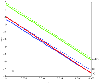
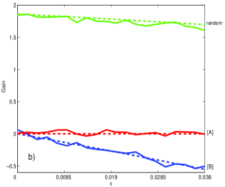
Figure 4: Comparison of the theoretical rates of winning – dashed lines – together with the rates obtained through simulations – solid lines. All the simulations were obtained by averaging over $50\,000$ trials and over all possible initial conditions. a) The parameters correspond to the ones used in equations (4.1). b) The parameters correspond to the ones used in equations (4.1).

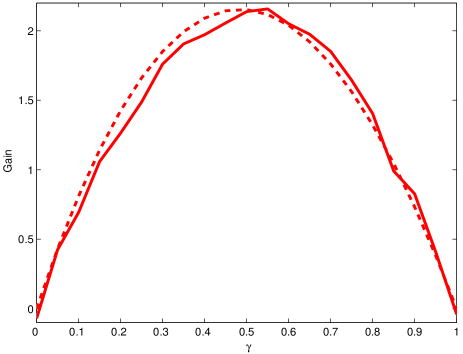
Figure 5: Comparison between the theoretical and the simulation for the gain vs gamma, for the following set of probabilities : $p=\frac{1}{3}$, $r=\frac{1}{3}$; $p_{1}=\frac{3}{25}$, $r_{1}=\frac{2}{5}$ and $p_{2}=\frac{3}{5}$, $r_{2}=\frac{1}{10}$. The simulations were carried out by averaging over $50\,000$ trials and all possible initial conditions.

The performance of the random alternation is more variable, obtaining in some cases a greater gain than in the deterministic cases – see figure 3c.

In figures (4a) and (4b) a comparison between the theoretical rates of winning for games A, B and AB given by (4.1) and (4.1) and the rates obtained through simulations is presented. It is worth noting the good agreement between both results.

It is also interesting to see how evolves the average gain obtained from the random alternation of game A and game B when varying the mixing parameter $\gamma$. In figure 5 we compare both the experimental and theoretical curves. As in the original games, the maximum gain is obtained for a value around $\gamma\sim\frac{1}{2}$ (Lee et al. 2002b).

5 Conclusion

We have reviewed how the derivation of Parrondo’s games from the flashing Brownian ratchet can be rigorously established via the Fokker-Planck equation. This procedure reveals new Parrondo games, of which the original Parrondo games are a special case with self-transitions set to zero. This confirms Parrondo’s original intuition based on a flashing ratchet is correct with rigour. We interpreted the self-transitions in terms of particles, in the flashing ratchet, that remain stationary in a given cycle. We then presented a new DTMC analysis for the new games showing that Parrondo’s paradox still occurs if the appropriate conditions are fulfilled. New expressions for the rates of winning have been obtained, with the result that within certain conditions a higher rate of winning than in the original games can be obtained. We have also studied how the parameter space where the paradox exists changes with the self-transition variables, and conclude that the parameter space corresponding to the original Parrondo’s games is a limiting case of the maximum volume – as the self-transition probabilities increase in value the volume shrinks to zero. However, it is worth noting that despite the volume decreases with increasing the self-transition probabilities, the rates of winning that can be obtained are higher than in the original Parrondo’s games.

This work was supported by GTECH Australasia; the Ministerio de Ciencia y Tecnología (Spain) and FEDER, projects BFM2001-0341-C02-01 and BFM2000-1108; P.A. acknowledges support form the Govern Balear, Spain.

References

- [1] Abbott, D. 2001 Overview: Unsolved problems of noise and fluctuations. Chaos 11, 526–538.
- [2] Abbott, D., Davies, P.C.W. & Shalizi, C. R. 2002 Order from disorder: the role of noise in creative processes. Fluctuation and Noise Letters 2, C1–C12.
- [3] Adjari, A. & Prost, J. 1993 Drift induced by a periodic potential of low symmetry: pulsed dielectrophoresis. C. R. Academy of Science Paris, Série II 315, 1635–1639.
- [4] Ait-Haddou, R. & Herzog, W. 2002 Force and motion generation of myosin motors: muscle contraction. J. Electromyography and Kinesiology 12, 435–445.
- [5] Allison, A. & Abbott, D. 2001a Control systems with stochastic feedback. Chaos 11, 715–724.
- [6] Allison, A. & Abbott, D. 2001b Stochastic resonance on a Brownian ratchet. Fluctuation and Noise Letters 1, L239- L244.
- [7] Allison, A., & Abbott, D. 2002 The physical basis for Parrondo’s games. Fluctuation and Noise Letters 2, L327–L342.
- [8] Arena, P., Fazzino, S., Fortuna, L. & Maniscalco, P. 2003 Game theory and non-linear dynamics: the Parrondo paradox case study. Chaos, Solitons and Fractals 17, 545–555.
- [9] Boman, M., Johansson, S. J. & Lyback, D. 2001 Parrondo strategies for artificial traders. Intelligent Agent Technology (eds. N. Zhong, J. Liu, S. Ohsuga & J. Bradshaw), 150–159. World Scientific. Also available at cs/0 204 051.
- [10] Buceta, J., Lindenberg, K. & Parrondo, J. M. R. 2002a Spatial patterns induced by random switching. Fluctuation and Noise Letters 2, L21 -L29.
- [11] Buceta, J., Lindenberg, K. & Parrondo, J. M. R. 2002b Pattern formation induced by nonequilibrium global alternation of dynamics. Physical Review E 66, 036 216(11).
- [12] Buceta, J. & Lindenberg, K. 2002 Switching-induced Turing instability. Physical Review E 66, 046 202(4).
- [13] Cleuren, B. & Van den Broeck, C. 2002 Random walks with absolute negative mobility. Physical Review E 65, 030 101(4).
- [14] Davies, P. C. W. 2001 Physics and life: the Abdus Salam memorial lecture, in Sixth Trieste Conference on Chemical Evolution, Trieste, Italy (eds. J. Chela-Flores, T. Tobias & F. Raulin), 13- 20. Kluwer Academic Publishers.
- [15] Dinis, L. & Parrondo, J. M. R. 2002 Parrondo’s paradox and the risks of short-range optimization. Preprint cond-mat/0 212 358.
- [16] Flitney, A. P., Ng, J. & Abbott, D. 2002 Quantum Parrondo’s games. Physica A 314, 35–42.
- [17] Harmer, G. P. & Abbott, D. 1999a Parrondo’s paradox. Statistical Science 14, 206–213.
- [18] Harmer, G. P. & Abbott, D. 1999b Losing strategies can win by Parrondo’s paradox. Nature 402, 864.
- [19] Harmer, G. P., Abbott, D. & Taylor, P. G. 2000 The paradox of Parrondo’s games. Proc. R. Soc. London A 456, 247–259.
- [20] Harmer, G. P., Abbott, D., Taylor, P. G. & Parrondo, J. M. R. 2001 Brownian ratchets and Parrondo’s games. Chaos 11, 705–714.
- [21] Harmer, G. P. & Abbott, D. 2002 A review of Parrondo’s paradox. Fluctuation and Noise Letters 2, R71–R107.
- [22] Heath, D., Kinderlehrer, D. & Kowalczyk, M. 2002 Discrete and continuous ratchets: from coin toss to molecular motor. Discrete and Continuous Dynamical Systems-Series B 2, 153–167.
- [23] Horsthemke, W. & Lefever, R. 1984 Noise–induced transitions: theory and applications in Physics, Chemistry and Biology. Springer–Verlag. Berlin.
- [24] Karlin, S. 1973 A first course in stochastic processes. Academic Press. New York.
- [25] Kay, R. J. & Johnson, N. F. 2002 Winning combinations of history-dependent games. Preprint cond-mat/0 207 386.
- [26] Kestenbaum, D. 1997 Sand castles and cocktail nuts. New Scientist 154, 25 -28.
- [27] Key, E. S. 1987 Computable examples of the maximal Lyapunov exponent. Probab. Th. Rel. Fields 75, 97–107.
- [28] Key, E. S., Kłosek, M. & Abbott, D. 2002 On Parrondo’s paradox: how to construct unfair games by composing fair games. Preprint math/0 206 151.
- [29] Kinderlehrer, D. & Kowalczyk, M. 2002 Diffusion-mediated transport and the flashing ratchet. Archive for Rational Mechanics and Analysis 161, 149-179.
- [30] Kocarev, L. & Tasev, Z. 2002 Lyapunov exponents, noise-induced synchronization, and Parrondo’s paradox. Physical Review E 65, 046 215(4).
- [31] Latouche, G. & Taylor, P.G. 2003 Drift conditions for matrix-analytic models. Mathematics of Operations Research 28, 346–360.
- [32] Lee, C. F., Johnson, N. F., Rodriguez, F. & Quiroga, L. 2002a Quantum coherence, correlated noise and Parrondo games. Fluctuation and Noise Letters 2, L293–L298.
- [33] Lee, Y., Allison, A., Abbott, D. & Stanley, H. E. 2002b Minimal Brownian ratchet: an exactly solvable model. Submitted to Physical Review Letters. Also available at cond-mat/0 205 302.
- [34] Mihailović, Z. & Rajković, M. 2003a One dimensional asynchronous cooperative Parrondo’s games. Preprint cond-mat/0 307 193.
- [35] Mihailović, Z. & Rajković, M. 2003b Synchronous cooperative Parrondo’s games. Preprint cond-mat/0 307 212.
- [36] Maslov, S. & Zhang, Y. 1998 Optimal investment strategy for risky assests. Int. J. of Th. and Appl. Finance 1, 377–387.
- [37] Meyer, D. A. & Blumer, H. 2002a Quantum Parrondo games: biased and unbiased. Fluctuation and Noise Letters 2, L257–L262.
- [38] Meyer, D. A. & Blumer, H. 2002b Parrondo games as a lattice gas automata. J. Stat. Phys. 107, 225- 239.
- [39] Moraal, H. 2000 Counterintuitive behaviour in games based on spin models. J. Phys. A: Math. Gen. 33, L203–L206.
- [40] Parrondo, J. M. R. 1996 How to cheat a bad mathematician. EEC HC&M Network on Complexity and Chaos (#ERBCHRX-CT 940 546), Torino, Italy. Unpublished.
- [41] Parrondo, J. M. R., Harmer, G. P. & Abbott, D. 2000 New paradoxical games based on Brownian ratchets. Physical Review Letters 85, 5226–5229.
- [42] Percus, O. E. & Percus, J. K. 2002 Can two wrongs make a right? Coin-tossing games and Parrondo’s paradox. Mathematical Intelligencer 24, 68–72.
- [43] Pinsky, R. & Scheutzow, M. 1992 Some remarks and examples concerning the transient and recurrence of random diffusions. Annales de l’Institut Henri Poincaré – Probabilités et Statistiques 28, 519–536.
- [44] Pyke, R. 2002 On random walks related to Parrondo’s games. Preprint math/0 206 150.
- [45] Reimann, P. 2002 Brownian motors: noisy transport far from equilibrium. Physics Reports 361, 57–265.
- [46] Rosato, A., Strandburg, K. J., Prinz, F. & Swendsen, R. H. 1987 Why the Brazil nuts are on top: size segregation of particulate matter by shaking. Physical Review Letters 58, 1038–1040.
- [47] Toral, R. 2001 Cooperative Parrondo’s games. Fluctuations and Noise Letters 1, L7–L12.
- [48] Toral, R. 2002 Capital redistribution brings wealth by Parrondo’s paradox. Fluctuations and Noise Letters 2, L305–L311.
- [49] Toral, R., Amengual, P. & Mangioni, S. 2003a Parrondo’s games as a discrete ratchet. Accepted in Physica A, avaliable also at cond-mat/0 302 424.
- [50] Toral, R., Amengual, P. & Mangioni, S. 2003b A Fokker-Planck description for Parrondo’s games. Proc. SPIE Noise in complex systems and stochastic dynamics (eds. L. Schimansky–Geier, D. Abbott, A. Neiman & C. Van den Broeck), 5114, 309–317. Santa Fe.
- [51] Westerhoff, H. V., Tsong, T. Y., Chock, P. B., Chen, Y. & Astumian, R. D. 1986 How enzymes can capture and transmit free energy contained in an oscillating electric field. Proc. Natl. Acad. Sci. 83, 4734–4738.