LANDAU EXPANSION FOR THE KUGEL-KHOMSKII $t_{2g}$ HAMILTONIAN

Abstract

The Kugel-Khomskii (KK) Hamiltonian for the titanates describes spin and orbital superexchange interactions between $d^{1}$ ions in an ideal perovskite structure in which the three $t_{2g}$ orbitals are degenerate in energy and electron hopping is constrained by cubic site symmetry. In this paper we implement a variational approach to mean-field theory in which each site, $i$, has its own $n\times n$ single-site density matrix ${\mbox{\boldmath{$\rho$}}}(i)$, where $n$, the number of allowed single-particle states, is 6 (3 orbital times 2 spin states). The variational free energy from this 35 parameter density matrix is shown to exhibit the unusual symmetries noted previously which lead to a wavevector-dependent susceptibility for spins in $\alpha$ orbitals which is dispersionless in the $q_{\alpha}$-direction. Thus, for the cubic KK model itself, mean-field theory does not provide wavevector ‘selection’, in agreement with rigorous symmetry arguments. We consider the effect of including various perturbations. When spin-orbit interactions are introduced, the susceptibility has dispersion in all directions in ${\bf q}$-space, but the resulting antiferromagnetic mean-field state is degenerate with respect to global rotation of the staggered spin, implying that the spin-wave spectrum is gapless. This possibly surprising conclusion is also consistent with rigorous symmetry arguments. When next-nearest-neighbor hopping is included, staggered moments of all orbitals appear, but the sum of these moments is zero, yielding an exotic state with long-range order without long-range spin order. The effect of a Hund’s rule coupling of sufficient strength is to produce a state with orbital order.

I INTRODUCTION

High temperature superconductivity[1] and colossal magnetoresistance[2] have sparked much recent interest in the magnetic properties of transition metal oxides, particularly those with orbital degeneracy.[3, 4] In many transition metal oxides, the $d$ electrons are localized due to the very large on-site Coulomb interaction, $U$. In cubic oxide perovskites, the crystal field of the surrounding oxygen octahedra splits the $d$-orbitals into a two-fold degenerate $e_{g}$ and a three-fold degenerate $t_{2g}$ manifold. In most cases, these degeneracies are further lifted by a cooperative Jahn-Teller (JT) distortion,[3] and the low energy physics is well described by an effective superexchange spin-only model. [5, 6, 7] However, some perovskites, such as LaTiO₃,[8, 9] do not undergo a significant JT distortion, in spite of the orbital degeneracy.[10] In these systems, the effective superexchange model must deal with not only the spin degrees of freedom but also the degenerate orbital degrees of freedom.[3, 4, 11] The large degeneracy of the resulting ground states may then yield rich phase diagrams, with exotic types of order, involving a strong interplay between the spin and orbital sectors.[4, 8, 9]

In the idealized cubic model for the titanates, there is one $d$ electron in the $t_{2g}$ degenerate manifold, which contains the wavefunctions $|X\rangle\equiv d_{yz}$, $|Y\rangle\equiv d_{xz}$, and $|Z\rangle\equiv d_{xy}$. Following Kugel and Khomskii (KK),[11] one starts from a Hubbard model with on-site Coulomb energy $U$ and nearest-neighbor (nn) hopping energy $t$. For large $U$, this model can be reduced to an effective superexchange model, which involves only nn spin and orbital coupling, with energies of order $\epsilon=t^{2}/U$. This low energy model has been the basis for several theoretical studies of the titanates. In particular, it has been suggested [12] that the KK Hamiltonian gives rise to an ordered isotropic spin phase, and that an energy gap in the spin excitations can be caused by spin-orbit interactions.[13] However, these papers are based on assumptions and approximations which are hard to assess. Recently[14] (this will be referred to as I) we have presented rigorous symmetry arguments which show several unusual symmetries of the cubic KK Hamiltonian. Perhaps the most striking symmetry is the rotational invariance of the total spin of $\alpha$ orbitals (where $\alpha=X,Y$, or $Z$) summed over all sites in a plane perpendicular to the $\alpha$-axis. This symmetry implies that in the disordered phase the wavevector-dependent spin susceptibility for $\alpha$ orbitals, $\chi_{\alpha}({\bf q})$ is dispersionless in the $q_{\alpha}$-direction. In addition, as discussed in I, this symmetry implies that the system does not support long-range spin order at any nonzero temperature. Thus the idealized cubic KK model is an inappropriate starting point to describe the properties of existing titanate systems. This peculiar rotational invariance depends on the special symmetry of the hopping matrix element and it can be broken by almost any perturbation such as rotation of the oxygen octahedra. Here we consider the effect of symmetry-breaking perturbations due to a) spin-orbit interactions, b) next-nearest-neighbor (nnn) hopping, and c) Hund’s rule coupling. According to the general symmetry argument of I, although long-range order at nonzero temperature is possible when spin-orbit interactions are included, the system still possesses enough rotation symmetry that the excitation spectrum should be gapless. (This conclusion is perhaps surprising because once spin-orbit interactions are included, the system might be expected to distinguish directions relative to those defined by the lattice.) This argument would imply that mean-field theory will produce a state which has a continuous degeneracy associated with global rotation of the spins. The purpose of this paper is to implement mean-field theory and to interpret the results obtained therefrom in light of the general symmetry arguments. We will carry out this analysis using the variational properties of the density matrix. In a separate paper[15] (which we will refer to as III, the present paper being paper II) we will study the self-consistent equations of mean-field theory which contain information equivalent to what we obtain here, but in a form which is better suited to a study of the ordered phase. Here our analysis is carried out for the cubic KK Hamiltonian with and without the inclusion of the symmetry-breaking perturbations mentioned above. In the presence of spin-orbit interactions we find that the staggered moments of different orbital states are not collinear, so that the net spin moment is greatly reduced from its spin-only value. The effect of nnn hopping is also interesting. Within mean-field theory, this perturbation was found to stabilize a state having long-range staggered spin order for each orbital state, but the staggered spins of the three orbital states add to zero. When only Hund’s rule coupling is included, mean-field theory predicts stabilization of long-range spin and orbital order. However, elsewhere[16] we show that fluctuations favor spin-only order. As a result, a state with long-range order of both spin and orbital degrees of freedom can only occur when the strength of the Hund’s rule coupling exceeds some critical value which we can not estimate in the present formalism.

Briefly this paper is organized as follows. In Sec. II we discuss the KK Hamiltonian and fix the notation we will use. In Sec. III we discuss the construction of the mean-field trial density matrix as the product of single-site density matrices, each of which acts on the space of six one-electron states of an ion, and whose parametrization therefore requires 35 parameters. Here we show that the wavevector-dependent spin susceptibilities which diverge as the temperature is lowered through a critical value have dispersionless directions, so that unusually mean-field theory provides no ‘wavevector selection’ at the mean-field transition. In Sec. IV we discuss the Landau expansion at quartic order. In Sec. V we treat several lower symmetry perturbations, namely spin-orbit interactions, nnn hopping, and Hund’s rule coupling. In each of these cases ‘wavevector selection’ leads to the usual two-sublattice structure, but the qualitative nature of ordering depends on which perturbation is considered. In Sec. VI we summarize our work and discuss its implications.

II THE HAMILTONIAN

The system we treat is a simple cubic lattice of ions with one d electron per ion in a d-band whose five orbital states are split into an $e_{g}$ doublet at high energy and a $t_{2g}$ triplet at low energy. Following the seminal work of Kugel and Khomskii[11] (KK), we describe this system by a Hubbard Hamiltonian ${\cal H}_{H}$ of the form

$${\cal H}_{H} = \sum_{i\alpha\sigma}\epsilon_{\alpha}c_{i\alpha\sigma}^{\dagger}c_{i\alpha\sigma}+\sum_{\langle ij\rangle}\sum_{\alpha\beta\sigma}t_{\alpha\beta}(i,j)c_{i\alpha\sigma}^{\dagger}c_{j\beta\sigma}$$ (2)

$$\ +U\sum_{i}\sum_{\alpha\leq\beta}\sum_{\sigma\sigma^{\prime}}c_{i\alpha\sigma}^{\dagger}c_{i\alpha\sigma}c_{i\beta\sigma^{\prime}}^{\dagger}c_{i\beta\sigma^{\prime}}\ ,$$

where $c_{i\alpha\sigma}^{\dagger}$ creates an electron in the orbital labeled $\alpha$ in spin state $\sigma$ on site $i$, $\epsilon_{\alpha}$ is the crystal field energy of the $\alpha$ orbital, $t_{\alpha\beta}(i,j)$ is the matrix element for hopping between orbital $\alpha$ of site $i$ and orbital $\beta$ of site $j$, and $\langle ij\rangle$ indicates that the sum is over pairs of nearest neighboring sites $i$ and $j$ on a simple cubic lattice. It is convenient to refer to the orbital state of an electron as its ‘flavor’. In this terminology $c_{i\alpha\sigma}^{\dagger}$ creates an electron of flavor $\alpha$ and $z$-component of spin $\sigma$ on site $i$. Initially we consider the case when the Coulomb interaction does not depend on which orbitals the electrons are in. In a later section we will consider the effects of Hund’s-rule coupling. In a cubic crystal field, the crystal-field energy $\epsilon_{\alpha}$ splits the five orbital d states into a low-energy triplet, whose states are $d_{yz}\equiv X$, $d_{xz}\equiv Y$, and $d_{xy}\equiv Z$, and a high energy doublet, whose presence is ignored. In this model it is assumed that hopping occurs only between nearest neighbors and proceeds via superexchange through an intervening oxygen $p$ orbital, so that the symmetry of the hopping matrix is that illustrated in Fig. 1. Thus $t_{\alpha\beta}$ is zero if $\alpha\not=\beta$ and $t_{\alpha\alpha}(i,j)=t$, except that $t_{\alpha\alpha}(i,j)$ vanishes if the bond $\langle ij\rangle$ is parallel to the $\alpha$-axis.[11] The $\alpha$-axis is called[17] the inactive axis for hopping between $\alpha$ orbitals. When $t\ll U$, KK reduced the above Hubbard Hamiltonian to an effective Hamiltonian for the manifold of states for which each site has one electron in a $t_{2g}$ orbital state. We will call this low-energy Hamiltonian the KK Hamiltonian and it can be regarded as a many-band generalization of the Heisenberg Hamiltonian. The KK Hamiltonian is often written in terms of spin variables to make the analogy with the Heisenberg model more apparent, but for our purposes it is more convenient to write the (KK) Hamiltonian in the form

$${\cal H}_{KK} = \epsilon\sum_{\langle ij\rangle}\sum_{\beta\gamma\not=\langle ij\rangle}\sum_{\eta\rho}c_{i\beta\eta}^{\dagger}c_{i\gamma\rho}c_{j\gamma\rho}^{\dagger}c_{j\beta\eta}$$ (3)

$$\equiv \ \epsilon\sum_{\langle ij\rangle}\sum_{\beta\gamma\not=\langle ij\rangle}\sum_{\eta\rho}Q_{\beta\eta;\gamma\rho}(i)Q_{\gamma\rho;\beta\eta}(j)\ ,$$ (4)

where $\epsilon=t^{2}/U$ and the notation $\beta\gamma\not=\langle ij\rangle$ indicates that in the sum over $\beta$ and $\gamma$ neither of these are allowed to be the same as the coordinate direction of the bond $\langle ij\rangle$.

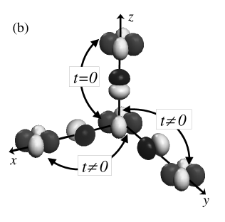
FIG. 1.: A schematic view of the $|Z\rangle=d_{xy}$ orbitals and the (indirect) hopping parameter $t$ via intermediate oxygen p-orbitals. Positive (negative) regions of wavefunctions are represented by dark (light) lobes. In (a) we show that the hopping matrix elements between orbitals of different flavors are zero. In (b) we show that there is no indirect hopping along the z-axis for an electron in the Z-orbital, due to symmetry.

Previously[14] we pointed out several unusual symmetries of this Hamiltonian. By an $\alpha$-plane we mean any plane perpendicular to the $\alpha$ axis (which is the inactive axis for $\alpha$-hopping). In I we showed that the total number of electrons in an $\alpha$-plane which are in $\alpha$ orbitals is constant. In addition, the total spin vector (as well as its $z$ component) summed over all electrons in $\alpha$ orbitals in any given $\alpha$-plane was shown to be a good quantum number. The fact that one can rotate the spin of all $\alpha$ electrons (these are electrons in $\alpha$ orbitals) in any $\alpha$-plane at no cost in energy implies that there is no long-range spin order at any nonzero temperature.[14] Nevertheless, since experiment[8] shows that LaTiO₃ does exhibit long-range spin order, it must be that spin ordering is caused by some, possibly small, symmetry breaking perturbation, which should be added to the idealized KK model. Therefore it is worthwhile investigating what form of long-range order results when possible symmetry-breaking perturbations are included. Although the mean-field results we obtain below should not be taken quantitatively, they may form a qualitative guide to the type of ordering one might expect for more realistic extensions of the above KK model. We also noted[6, 14] that even when spin-orbit coupling is included, the Hamiltonian has sufficient symmetry that the spin-wave spectrum remains gapless. As a result, the gap observed[8] in the excitation spectrum of LaTiO₃ can not be explained on the basis of the KK Hamiltonian with only the spin-orbit interaction as a perturbation. As we shall see, these symmetries are realized by the mean-field solutions we obtain.

III LANDAU EXPANSION AT QUADRATIC ORDER

We will develop the Landau expansion of the free energy as a multivariable expansion in powers of the full set of order parameters necessary to describe the free energy arising from the KK Hamiltonian. In this section we construct this expansion up to quadratic order in these order parameters and thereby analyze the instability of the disordered phase relative to arbitrary types of long-range order. In later sections we discuss how this picture is modified by higher-order terms in the expansion, and by the addition of various symmetry-breaking terms into the Hamiltonian.

A Parametrizing the Density Matrix

The version of mean-field theory which we will implement is based on the variational principle according to which the exact free energy is obtained by minimizing the free energy functional $F({\mbox{\boldmath{$\rho$}}})$ as a function of the trial density matrix $\rho$, which must be Hermitian, have no negative eigenvalues, and be normalized by ${\rm Tr}{\mbox{\boldmath{$\rho$}}}=1$. Here the trial free energy is

$$F({\mbox{\boldmath{$\rho$}}}) = {\rm Tr}\Bigl{[}{\mbox{\boldmath{$\rho$}}}\bigl{(}{\cal H}+kT\ln{\mbox{\boldmath{$\rho$}}}\bigr{)}\Bigr{]},$$ (5)

where the first term is the trial energy and the second is $-T$ times the trial entropy, where $T$ is the temperature. Mean-field theory is obtained by the ansatz that $\rho$ is the product of single-site density matrices, ${\mbox{\boldmath{$\rho$}}}(i)$:

$${\mbox{\boldmath{$\rho$}}}=\prod_{i}{\mbox{\boldmath{$\rho$}}}(i),$$ (6)

and $F({\mbox{\boldmath{$\rho$}}})$ is then minimized with respect to the variables used to parametrize the density matrix, ${\mbox{\boldmath{$\rho$}}}(i)$. Since ${\mbox{\boldmath{$\rho$}}}(i)$ acts in the space of $t_{2g}$ states of one electron, it is a $6\times 6$ dimensional Hermitian matrix with unit trace.

The most general trial density matrix (for site $i$) can be written in the form

$${\mbox{\boldmath{$\rho$}}}(i)=\frac{1}{6}{\cal I}+X(i),$$ (7)

where

$$X(i)=\sum_{\alpha\beta}\sum_{\rho\eta}c^{\dagger}_{i\alpha\rho}Y_{\alpha\rho\beta\eta}(i)c_{i\beta\eta}\ ,$$ (8)

with

$$Y_{\alpha\rho\beta\eta}(i)={\bf A}_{\alpha\beta}(i)\delta_{\rho\eta}+\vec{\bf B}_{\alpha\beta}(i)\cdot\vec{{\mbox{\boldmath{$\sigma$}}}}_{\rho\eta}\ .$$ (9)

Here $\vec{{\mbox{\boldmath{$\sigma$}}}}$ is the Pauli matrix vector, and ${\bf A}_{\alpha\beta}(i)$, ${\bf B}^{x}_{\alpha\beta}(i)$, ${\bf B}^{y}_{\alpha\beta}(i)$, and ${\bf B}^{z}_{\alpha\beta}(i)$ are $3\times 3$ Hermitian matrices, of which the first is traceless. The diagonal terms of the matrix ${\bf A}$ are parametrized for later convenience as

$${\bf A}_{xx}(i)=\frac{a_{1}(i)}{\sqrt{6}} + \frac{a_{2}(i)}{\sqrt{2}},\ \ {\bf A}_{yy}(i)=\frac{a_{1}(i)}{\sqrt{6}}-\frac{a_{2}(i)}{\sqrt{2}},$$ (10)

$${\bf A}_{zz}(i) = -{\mbox{\boldmath{$A$}}}_{xx}(i)-{\mbox{\boldmath{$A$}}}_{yy}(i),$$ (11)

such that

$${\mbox{\boldmath{$A$}}}_{xx}^{2}(i)+{\mbox{\boldmath{$A$}}}_{yy}^{2}(i)+{\mbox{\boldmath{$A$}}}_{xzz}^{2}(i) = a_{1}^{2}(i)+a_{2}^{2}(i),$$ (12)

$$-{\mbox{\boldmath{$A$}}}_{xx}^{2}(i)-{\mbox{\boldmath{$A$}}}_{yy}^{2}(i)+2{\mbox{\boldmath{$A$}}}_{zz}^{2}(i) = a_{1}^{2}(i)-a_{2}^{2}(i).$$ (13)

For any operator ${\cal O}(i)$ associated with site $i$ we define

$$\langle{\cal O}(i)\rangle\equiv{\rm Tr}[{\cal O}(i){\mbox{\boldmath{$\rho$}}}]\ ,$$ (14)

where Tr denotes a trace over the six states $|\alpha,\sigma\rangle$ of the atom at site $i$ with a single $t_{2g}$ electron. Then the diagonal matrix elements of ${\bf A}(i)$ give the occupations of orbital states,

$$\langle N_{\alpha}(i)\rangle=\langle\sum_{\sigma}c_{i\alpha\sigma}^{\dagger}c_{i\alpha\sigma}\rangle=2{\mbox{\boldmath{$A$}}}_{\alpha\alpha}(i),$$ (15)

which may be related to the matrix elements of the angular momentum, $L$,

$$\langle\frac{L_{x}^{2}(i)-1}{3}\rangle=\langle N_{x}(i)\rangle = {1\over 3}+{2\over\sqrt{6}}a_{1}(i)+\sqrt{2}a_{2}(i),$$ (16)

$$\langle\frac{L_{y}^{2}(i)-1}{3}\rangle=\langle N_{y}(i)\rangle = {1\over 3}+{2\over\sqrt{6}}a_{1}(i)-\sqrt{2}a_{2}(i),$$ (17)

$$\langle\frac{L_{z}^{2}(i)-1}{3}\rangle=\langle N_{z}(i)\rangle = {1\over 3}-{4\over\sqrt{6}}a_{1}(i)\ .$$ (18)

The off-diagonal matrix elements of ${\bf A}(i)$ are

$$\langle L_{\gamma}(i)\rangle = i\sum_{\alpha\beta}\sum_{\sigma}\langle c_{i\alpha\sigma}^{\dagger}c_{i\beta\sigma}\rangle\epsilon_{\alpha\beta\gamma}$$ (19)

$$= -2i\sum_{\alpha\beta}{\mbox{\boldmath{$A$}}}_{\alpha\beta}(i)\epsilon_{\alpha\beta\gamma},$$ (20)

where $\epsilon_{\alpha\beta\gamma}$ is the fully antisymmetric tensor. Similarly,

$$\langle L_{\beta}(i)L_{\gamma}(i)+L_{\gamma}(i)L_{\beta}(i)\rangle = -3\sum_{\sigma}\langle c_{i\beta\sigma}^{\dagger}c_{i\gamma\sigma}+c^{\dagger}_{i\gamma\sigma}c_{i\beta\sigma}\rangle$$ (21)

$$= -6[{\mbox{\boldmath{$A$}}}_{\beta\gamma}(i)+{\mbox{\boldmath{$A$}}}_{\gamma\beta}(i)].$$ (22)

Similarly, the diagonal matrix elements of ${\bf B}^{\gamma}(i)$, ${\bf B}^{\gamma}_{\alpha\alpha}(i)$, give the thermal expectation value of the $\gamma$ component of the spin of $\alpha$-flavor electrons:

$$\langle S_{\alpha\gamma}(i)\rangle = \sum_{\sigma\eta}\langle c_{i\alpha\sigma}^{\dagger}{\mbox{\boldmath{$\sigma$}}}_{\sigma\eta}^{\gamma}c_{i\alpha\eta}\rangle\ =2{\bf B}^{\gamma}_{\alpha\alpha}(i).$$ (23)

The off-diagonal matrix elements of ${\bf B}^{\gamma}(i)$ are related to the order-parameters associated with correlated ordering of spins and orbits.

In general, the density matrix Eq. (7) yields the average

$$\langle Q_{\alpha\sigma;\beta\eta}(i)\rangle\equiv\langle c_{i\alpha\sigma}^{\dagger}c_{i\beta\eta}\rangle=\frac{1}{6}\delta_{\alpha\beta}\delta_{\sigma\eta}$$ (24)

$$+ \sum_{\stackrel{{\scriptstyle\alpha^{\prime}\beta^{\prime}}}{{\rho\tau}}}\langle c^{\dagger}_{i\alpha\sigma}c_{i\beta\eta}c^{\dagger}_{i\alpha^{\prime}\rho}({\bf A}_{\alpha^{\prime}\beta^{\prime}}(i)\delta_{\rho\tau}+\vec{\bf B}_{\alpha^{\prime}\beta^{\prime}}(i)\cdot\vec{{\mbox{\boldmath{$\sigma$}}}}_{\rho\tau})c_{i\beta^{\prime}\tau}\rangle$$ (25)

$$= \delta_{\alpha\beta}\delta_{\sigma\eta}/6+{\bf A}_{\beta\alpha}(i)\delta_{\sigma\eta}+\vec{\bf B}_{\beta\alpha}(i)\cdot\vec{{\mbox{\boldmath{$\sigma$}}}}_{\eta\sigma}.$$ (26)

B Construction of the Trial Free Energy

Using the result Eq. (26), we get the trial energy, $U$, as

$$U=\ \epsilon\sum_{\langle ij\rangle}\sum_{\beta\gamma\not=\langle ij\rangle}\sum_{\eta\rho}\langle Q_{\beta\eta;\gamma\rho}(i)\rangle\langle Q_{\gamma\rho;\beta\eta}(j)\rangle$$ (27)

$$= 2\epsilon\sum_{\langle ij\rangle}\sum_{\alpha\beta\neq\langle ij\rangle}[{\mbox{\boldmath{$A$}}}_{\alpha\beta}(i){\mbox{\boldmath{$A$}}}_{\beta\alpha}(j)+\vec{{\mbox{\boldmath{$B$}}}}_{\alpha\beta}(i)\cdot\vec{{\mbox{\boldmath{$B$}}}}_{\beta\alpha}(j)],$$ (28)

where we have used the identity

$$\sum_{\rho_{2}}(\vec{{\mbox{\boldmath{$B$}}}}_{\alpha_{1}\alpha_{2}}\cdot\vec{{\mbox{\boldmath{$\sigma$}}}}_{\rho_{1}\rho_{2}})(\vec{{\mbox{\boldmath{$B$}}}}_{\alpha_{2}\alpha_{3}}\cdot\vec{{\mbox{\boldmath{$\sigma$}}}}_{\rho_{2}\rho_{3}})$$ (29)

$$= \vec{{\mbox{\boldmath{$B$}}}}_{\alpha_{1}\alpha_{2}}\cdot\vec{{\mbox{\boldmath{$B$}}}}_{\alpha_{2}\alpha_{3}}\delta_{\rho_{1}\rho_{3}}+i\vec{\sigma}_{\rho_{1}\rho_{3}}\cdot\vec{{\mbox{\boldmath{$B$}}}}_{\alpha_{1}\alpha_{2}}\times\vec{{\mbox{\boldmath{$B$}}}}_{\alpha_{2}\alpha_{3}}.$$ (30)

Here and below we drop terms independent of the trial order-parameters.

Using Eq. (7) we write the trial entropy as

$$-TS = kT\sum_{i}{\rm Tr}(3X^{2}(i)-6X^{3}(i)+18X^{4}(i)+\dots),$$ (31)

where we noted that ${\rm Tr}X(i)=0$. The second-order contribution is found from

$${\rm Tr}[X^{2}(i)]=\sum_{\stackrel{{\scriptstyle\alpha\beta}}{{\alpha^{\prime}\beta^{\prime}}}}\sum_{\stackrel{{\scriptstyle\eta\rho}}{{\eta^{\prime}\rho^{\prime}}}}{\rm Tr}[c^{\dagger}_{i\alpha\rho}Y_{\alpha\rho\beta\eta}(i)c_{i\beta\eta}$$ (33)

$$\times c^{\dagger}_{i\alpha^{\prime}\rho^{\prime}}Y_{\alpha^{\prime}\rho^{\prime}\beta^{\prime}\eta^{\prime}}(i)c_{i\beta^{\prime}\eta^{\prime}}]=\sum_{\alpha\beta}\sum_{\eta\rho}Y_{\alpha\rho\beta\eta}(i)Y_{\beta\eta\alpha\rho}(i)$$

$$= \sum_{\alpha\beta}[{\mbox{\boldmath{$A$}}}_{\alpha\beta}(i){\mbox{\boldmath{$A$}}}_{\beta\alpha}(i)+\vec{{\mbox{\boldmath{$B$}}}}_{\alpha\beta}(i)\cdot\vec{{\mbox{\boldmath{$B$}}}}_{\beta\alpha}(i)].$$ (34)

At quadratic order the trial free-energy, $F=F_{2}$, is thus

$$F_{2} = \frac{1}{2}\sum_{ij}\sum_{\alpha\beta}\chi^{-1}_{\alpha\beta}(i,j)[{\mbox{\boldmath{$A$}}}_{\alpha\beta}(i){\mbox{\boldmath{$A$}}}_{\beta\alpha}(j)$$ (36)

$$\ \ \ \ \ \ \ \ \ \ +\vec{{\mbox{\boldmath{$B$}}}}_{\alpha\beta}(i)\cdot\vec{{\mbox{\boldmath{$B$}}}}_{\beta\alpha}(j)],$$

where the inverse susceptibility is given by

$$\chi_{\alpha\beta}^{-1}(i,j)=12kT\delta_{ij}+2\epsilon\gamma_{ij}(1-\delta_{ij,\alpha})(1-\delta_{ij,\beta}).$$ (37)

Here $\gamma_{ij}$ is unity if sites $i$ and $j$ are nearest neighbors and is zero otherwise, and $\delta_{ij,\alpha}$ is unity if the bond $\langle ij\rangle$ is along the $\alpha$-direction and is zero otherwise.

C Stability Analysis - Wavevector Selection

We now carry out a stability analysis of the disordered phase. At quadratic order in the Landau expansion, possible phase transitions from the disordered phase to a phase with long-range order are signalled by the divergence of a susceptibility. Depending on the higher-than-quadratic order terms in the Landau expansion, such a transition may (or may not) be preempted by a first-order (discontinuous) phase transition. So mean-field theory is a simple and usually effective way to predict the nature of the ordered phase in systems where it may not be easy to guess it. To implement the stability analysis we diagonalize the inverse susceptibility matrix by going to Fourier transformed variables, whose generic definition is

$$F({\bf q}) = {1\over\sqrt{N}}\sum_{i}F({\bf r}_{i})e^{-i{\bf q}\cdot{\bf r}_{i}},\ \$$ (38)

$$F({\bf r}_{i}) = {1\over\sqrt{N}}\sum_{\bf q}F({\bf q})e^{i{\bf q}\cdot{\bf r}_{i}},$$ (39)

where $N$ is the total number of lattice sites. Then the free energy at quadratic order is $F_{2}=\sum_{\bf q}F_{2}({\bf q})$, where

$$F_{2} = \frac{1}{2}\sum_{\bf q}\sum_{\alpha\beta}\chi^{-1}_{\alpha\beta}({\bf q})[{\mbox{\boldmath{$A$}}}_{\alpha\beta}({\bf q}){\mbox{\boldmath{$A$}}}_{\beta\alpha}(-{\bf q})$$ (41)

$$\ \ \ \ \ \ \ \ \ \ \ +\vec{{\mbox{\boldmath{$B$}}}}_{\alpha\beta}({\bf q})\cdot\vec{{\mbox{\boldmath{$B$}}}}_{\beta\alpha}(-{\bf q})],$$

with

$$\chi^{-1}_{\alpha\beta}({\bf q})=12kT$$ (42)

$$+ 2\epsilon\sum_{{\bf R}_{nn}}e^{-i{\bf q}\cdot{\bf R}_{nn}}(1-\delta_{{\bf R}_{nn},a\hat{\alpha}})(1-\delta_{{\bf R}_{nn},a\hat{\beta}}),$$ (43)

where ${\bf R}_{nn}$ is a vector to a nearest-neighbor site, and $\hat{\alpha}$ is the unit vector in the $\alpha$-direction. We hence see that we have only two kinds of inverse susceptibilities, the one for the diagonal elements, namely

$$\chi^{-1}_{\alpha\alpha}({\bf q}) = 12kT+2\epsilon\sum_{{\bf R}_{nn}}e^{-i{\bf q}\cdot{\bf R}_{nn}}(1-\delta_{{\bf R}_{nn},a\hat{\alpha}})$$ (44)

$$= 12kT+2\epsilon\sum_{\beta\gamma}\epsilon_{\alpha\beta\gamma}^{2}(c_{\beta}+c_{\gamma}),$$ (45)

and the second for the off-diagonal matrix elements, namely

$$\chi^{-1}_{\alpha\beta}({\bf q})=12kT + 2\epsilon\sum_{{\bf R}_{nn}}e^{-i{\bf q}\cdot{\bf R}_{nn}}(1-\delta_{{\bf R}_{nn},a\hat{\alpha}}-\delta_{{\bf R}_{nn},a\hat{\beta}})$$ (46)

$$= 12kT+4\epsilon\sum_{\gamma}\epsilon_{\alpha\beta\gamma}^{2}c_{\gamma},$$ (47)

where $c_{\alpha}\equiv\cos(q_{\alpha}a)$.

At high temperature all the eigenvalues of the susceptibility matrix are finite and positive. As the temperature is reduced, one or more eigenvalues may become zero, corresponding to an infinite susceptibility. Usually this instability will occur at some value of wavevector (or more precisely at the star of some wavevector), and this set of wavevectors describes the periodicity of the ordered phase near the ordering transition. This phenomenon is referred to as ‘wavevector selection’. In addition, and we will later see several examples of this, the eigenvector associated with the divergent susceptibility contains information on the qualitative nature of the ordering. Here, a central question which the eigenvector addresses, is whether the ordering is in the spin sector, the orbital sector, or both sectors. If the unstable eigenvector is degenerate, one can usually determine the symmetries which give rise to Goldstone (gapless) excitations. (We will meet this situation in connection with our treatment of spin-orbit interactions.) In the present case, we see from Eqs. (45) and (47) that the instabilities (where an inverse susceptibility vanishes) first appear at $kT=2\epsilon/3$ for the diagonal susceptibilities. Consider first the susceptibilities for unequal occupations of the three orbital states. Making use of Eqs. (11) and (45), we write

$$\sum_{\alpha}\chi^{-1}_{\alpha\alpha}({\bf q}){\mbox{\boldmath{$A$}}}_{\alpha\alpha}({\bf q}){\mbox{\boldmath{$A$}}}_{\alpha\alpha}(-{\bf q})$$ (48)

$$= \left[\begin{array}[]{cc}a_{1}({\bf q})&a_{2}({\bf q})\end{array}\right]{\mbox{\boldmath{$\chi$}}}_{n}({\bf q})\left[\begin{array}[]{c}a_{1}(-{\bf q})\\ a_{2}(-{\bf q})\end{array}\right],$$ (52)

with the 2$\times$2 susceptibility matrix ${\mbox{\boldmath{$\chi$}}}_{n}$ given by

$$\chi^{-1}_{n,11}({\bf q}) = 12kT+\frac{2\epsilon}{3}\Bigl{(}5c_{x}+5c_{y}+2c_{z}\Bigr{)},$$ (53)

$$\chi^{-1}_{n,22}({\bf q}) = 12kT+2\epsilon\Bigl{(}c_{x}+c_{y}+2c_{z}\Bigr{)},$$ (54)

$$\chi^{-1}_{n,12}({\bf q}) = \chi^{-1}_{n,21}({\bf q})=\frac{2\epsilon}{\sqrt{3}}\Bigl{(}c_{y}-c_{x}\Bigr{)}.$$ (55)

The instability occurs for both eigenvalues of the inverse susceptibility matrix $\chi^{-1}_{n,\ell m}({\bf q})$, but only when the wavevector ${\bf q}$ assumes its antiferromagnetic value ${\bf Q}=(\pi,\pi,\pi)/a$ which leads to a two sub-lattice structure (see Fig. 2) called the “G” state. The two-fold degeneracy is the symmetry associated with rotations in occupation number space $\langle N_{x}\rangle$, $\langle N_{y}\rangle$, and $\langle N_{z}\rangle$ with the constraint that the sum of these occupation numbers is unity. (At quadratic order we do not yet feel the discrete cubic symmetry of the orbital states.) In contrast, the inverse spin susceptibility $\chi^{-1}_{\alpha\alpha}$ of Eq. (45) has a flat branch so that it vanishes for $kT=2\epsilon/3$ for any value of $q_{\alpha}$, when the two other components of ${\bf q}$ assume the antiferromagnetic value $\pi/a$. This wavevector dependence indicates that correlations in the spin susceptibility become long ranged in an $\alpha$-plane, but different $\alpha$-planes are completely uncorrelated. Note that beyond the fact that there is no wavevector selection in the spin susceptibility, one has complete rotational invariance in ${\mbox{\boldmath{$B$}}}^{\gamma}_{\alpha\alpha}({\bf q})$ for the components labeled by $\gamma$ independently for each orbital labeled $\alpha$. This result reflects the exact symmetry of the Hamiltonian with respect to rotation of the total spin in the $\alpha$ orbital summed over all spins in any single $\alpha$-plane.[14] If we restrict attention to the G wavevector ${\bf q}={\bf Q}$, we have complete rotational degeneracy in the 11 dimensional space consisting of the nine ${\mbox{\boldmath{$B$}}}^{\gamma}_{\alpha\alpha}({\bf Q})$ spin order-parameters and the two $a_{n}({\bf Q})$ occupational order-parameters. Thus at this level of approximation, we have O(11) symmetry! Most of this symmetry only holds at quadratic order in mean-field theory. As usual, we expect that fourth (and higher) order terms in the Landau expansion will generate anisotropies in this 11-dimensional space to lower the symmetry to the actual cubic symmetry of the system. As we will see, the anisotropy which inhibits the mixing of spin and orbit degrees of freedom is not generated by the quartic terms in the free energy. Perhaps unexpectedly, as we show elsewhere,[16] this anisotropy is only generated by fluctuations not accessible to mean-field theory.

FIG. 2.: The two sublattice “G” state which consists of two interpenetrating simple cubic lattices on each site of which the ions are in a given state, either A or B.

Dispersionless branches of order-parameter susceptibilities which lead to an infinite degeneracy of mean-field states, have been found in a variety of models,[18, 19, 20, 21] of which perhaps the most celebrated is that in the kagomé[22] and pyrochlore[23] systems. In almost all cases, the dispersionless susceptibility is an artifact of mean-field theory and does not represent a true symmetry of the full Hamiltonian. In such a case, the continuous degeneracy is lifted by fluctuations, which can either be thermal fluctuations[24] or quantum fluctuations.[25] Here we have a rather unusual case in that the spin susceptibility has a dispersionless direction (parallel to the inactive axis) which is the result of an exact true symmetry of the quantum Hamiltonian which persists even in the presence of thermal and quantum fluctuations.

IV LANDAU EXPANSION AT QUARTIC ORDER

To discuss the nature of the ordered state one may consider the self-consistent equations for the nonzero order-parameters which appear below the ordering temperature at $kT_{c}=2\epsilon/3$ and this is done in III. However, the types of possible ordering should also be apparent from the form of the anisotropy of the free energy in order-parameter space which first occurs in terms in the free energy which are quartic in the order-parameters. In principle, long-range order is only possible when we add to the Hamiltonian terms which destroy the symmetry whereby one can rotate arbitrarily planes of spins associated with a given orbital flavor. In the next section we study several perturbations which stabilize long-range order. Although the nature of the ordering depends on the perturbation, generically the resulting dispersion due to this symmetry-breaking perturbation stabilizes the G structure, so that the instabilities are confined to the wavevector ${\bf q}={\bf Q}$. In this section we implicitly assume this scenario.

Accordingly, we now evaluate all terms in the free energy which involve four powers of the critical variables ${\mbox{\boldmath{$B$}}}^{\gamma}_{\alpha\alpha}({\bf Q})$ and ${\mbox{\boldmath{$A$}}}_{\alpha\alpha}({\bf Q})$ at the wavevector associated with the assumed two sub-lattice, or G, structure. These terms arise from two mechanisms. The first contribution, which we denote $F_{4}^{(4)}$, arises from “bare” quartic terms in Eq. (31). The second type of contribution arises indirectly through $X^{3}(i)$ in Eq. (31). There we have contributions to the free energy which involve two critical variables and one noncritical variable (evaluated at zero wavevector). When the free energy is minimized with respect to this noncritical variable, we obtain contributions to the free energy which are quartic in the critical order-parameters and which we denote $F_{4}^{(3)}$.

A Bare Quartic Terms, $F_{4}^{(4)}$

The bare quartic terms are obtained from Eq. (A11), by taking into account only diagonal matrix elements of the matrices $A$ and $\vec{{\mbox{\boldmath{$B$}}}}$. Since the fourth-order term of the entropy is multiplied by 18$kT$, [see Eq. (31)], and we can safely put here 18$kT$=12$\epsilon$, we find that the bare quartic terms are given by

$$F_{4}^{(4)} = 24\epsilon\sum_{i}\sum_{\alpha}\Bigl{[}{\mbox{\boldmath{$A$}}}^{4}_{\alpha\alpha}(i)+6{\mbox{\boldmath{$A$}}}^{2}_{\alpha\alpha}(i)s_{\alpha}^{2}(i)+s_{\alpha}^{4}(i)\Bigr{]},$$ (56)

where we have denoted

$$s_{\alpha}^{2}(i)=({\mbox{\boldmath{$B$}}}_{\alpha\alpha}^{x}(i))^{2}+({\mbox{\boldmath{$B$}}}_{\alpha\alpha}^{y}(i))^{2}+({\mbox{\boldmath{$B$}}}_{\alpha\alpha}^{z}(i))^{2}.$$ (57)

Introducing Fourier transformed variables via Eq. (39) we thereby obtain terms quartic in the critical order parameters as

$$F_{4}^{(4)} = \frac{24\epsilon}{N}\sum_{\alpha}\Bigl{[}{\mbox{\boldmath{$A$}}}^{4}_{\alpha\alpha}+6{\mbox{\boldmath{$A$}}}_{\alpha\alpha}^{2}s_{\alpha}^{2}+s_{\alpha}^{4}\Bigr{]},$$ (58)

where now all order parameters are to be evaluated at wavevector ${\bf Q}$. Using for the matrix elements of $A$ the parametrization Eq. (11), we find

$$F_{4}^{(4)}={\epsilon\over N}\Bigl{\{}12(a_{1}^{2}+a_{2}^{2})^{2}+48\sqrt{3}a_{1}a_{2}(s_{x}^{2}-s_{y}^{2})$$ (59)

$$+ 48(a_{1}^{2}+a_{2}^{2})(s_{x}^{2}+s_{y}^{2}+s_{z}^{2})+24(s_{x}^{4}+s_{y}^{4}+s_{z}^{4})$$ (61)

$$\ \ \ \ \ \ -24(a_{1}^{2}-a_{2}^{2})(s_{x}^{2}+s_{y}^{2}-2s_{z}^{2})\Bigr{\}}.$$

B Induced Quartic Terms, $F_{4}^{(3)}$

To obtain the terms of this type, we first take from Eq. (A4) all the terms having diagonal matrix elements. Multiplying them by $-6kT=-4\epsilon$ [see Eq. (31)], we have

$$V_{3} = -8\epsilon\sum_{i\alpha}\Bigl{[}{\mbox{\boldmath{$A$}}}^{3}_{\alpha\alpha}(i)+3{\mbox{\boldmath{$A$}}}_{\alpha\alpha}(i)\vec{{\mbox{\boldmath{$B$}}}}_{\alpha\alpha}(i)\cdot\vec{{\mbox{\boldmath{$B$}}}}_{\alpha\alpha}(i)\Bigr{]}.$$ (62)

Next we insert here the Fourier transforms. The critical variables we treat here are the Fourier components at wavevector ${\bf Q}\equiv(\pi,\pi,\pi)/a$. When the wavevector is ${\bf Q}$, it will be left implicit. We indicate explicitly only those variables taken at zero wavevector. Then $V_{3}$ is given by

$$V_{3} = -\frac{24\epsilon}{\sqrt{N}}\sum_{\alpha}\Bigl{[}{\mbox{\boldmath{$A$}}}_{\alpha\alpha}(0)({\mbox{\boldmath{$A$}}}_{\alpha\alpha}^{2}+s_{\alpha}^{2})$$ (63)

$$+ 2\vec{{\mbox{\boldmath{$B$}}}}_{\alpha\alpha}(0)\cdot\vec{{\mbox{\boldmath{$B$}}}}_{\alpha\alpha}{\mbox{\boldmath{$A$}}}_{\alpha\alpha}\Bigr{]},$$ (64)

where we have used Eq. (57).

We now eliminate the noncritical variables at zero wavevector by minimizing the free energy with respect to them. We note that all the noncritical zero wavevector variables have the same susceptibility

$$\chi(0)=(12kT+8\epsilon)^{-1}=(16\epsilon)^{-1},$$ (65)

and therefore the function to minimize is

$$\tilde{V}_{3} = V_{3}+8\epsilon\sum_{\alpha}\Bigl{[}{\mbox{\boldmath{$A$}}}_{\alpha\alpha}^{2}(0)+\vec{{\mbox{\boldmath{$B$}}}}_{\alpha\alpha}(0)\cdot\vec{{\mbox{\boldmath{$B$}}}}_{\alpha\alpha}(0)\Bigr{]}.$$ (66)

The minimization procedure, allowing for the constraint $\sum_{\alpha}{\mbox{\boldmath{$A$}}}_{\alpha\alpha}(0)=0$, yields

$${\mbox{\boldmath{$B$}}}_{\alpha\alpha}^{\gamma}(0) = \frac{3}{\sqrt{N}}{\mbox{\boldmath{$B$}}}_{\alpha\alpha}^{\gamma}{\mbox{\boldmath{$A$}}}_{\alpha\alpha},$$ (67)

$${\mbox{\boldmath{$A$}}}_{xx}(0) = \frac{1}{2\sqrt{N}}\Bigl{(}2{\mbox{\boldmath{$A$}}}_{xx}^{2}+2s_{x}^{2}-{\mbox{\boldmath{$A$}}}_{yy}^{2}-s_{y}^{2}-{\mbox{\boldmath{$A$}}}_{zz}^{2}-s_{z}^{2}\Bigr{)},$$ (68)

$${\mbox{\boldmath{$A$}}}_{yy}(0) = \frac{1}{2\sqrt{N}}\Bigl{(}2{\mbox{\boldmath{$A$}}}_{yy}^{2}+2s_{y}^{2}-{\mbox{\boldmath{$A$}}}_{xx}^{2}-s_{x}^{2}-{\mbox{\boldmath{$A$}}}_{zz}^{2}-s_{z}^{2}\Bigr{)},$$ (69)

$${\mbox{\boldmath{$A$}}}_{zz}(0) = -{\mbox{\boldmath{$A$}}}_{xx}(0)-{\mbox{\boldmath{$A$}}}_{yy}(0).$$ (70)

Inserting these values into Eq. (66) yields the contribution $F_{4}^{(3)}$ to the free energy

$$F_{4}^{(3)}=-\frac{72\epsilon}{N}\sum_{\alpha}{\mbox{\boldmath{$A$}}}_{\alpha\alpha}^{2}s_{\alpha}^{2}-\frac{12\epsilon}{N}\Bigl{[}\sum_{\alpha}({\mbox{\boldmath{$A$}}}_{\alpha\alpha}^{2}+s_{\alpha}^{2})^{2}$$ (71)

$$- ({\mbox{\boldmath{$A$}}}_{xx}^{2}+s_{x}^{2})({\mbox{\boldmath{$A$}}}_{yy}^{2}+s_{y}^{2})-({\mbox{\boldmath{$A$}}}_{yy}^{2}+s_{y}^{2})({\mbox{\boldmath{$A$}}}_{zz}^{2}+s_{z}^{2})$$ (73)

$$\ \ \ \ \ \ \ \ \ -({\mbox{\boldmath{$A$}}}_{zz}^{2}+s_{z}^{2})({\mbox{\boldmath{$A$}}}_{xx}^{2}+s_{x}^{2})\Bigr{]},$$

which, upon inserting the parametrization (11) becomes

$$F_{4}^{(3)} = {\epsilon\over N}\Bigl{\{}-12\Bigl{(}\sum_{\alpha}s_{\alpha}^{2}\Bigr{)}^{2}+36\sum_{\alpha<\beta}s_{\alpha}^{2}s_{\beta}^{2}-3(a_{1}^{2}+a_{2}^{2})^{2}$$ (74)

$$- 36\sqrt{3}a_{1}a_{2}(s_{x}^{2}-s_{y}^{2})-24(a_{1}^{2}+a_{2}^{2})(s_{x}^{2}+s_{y}^{2}+s_{z}^{2})$$ (76)

$$\ \ \ \ \ \ \ \ +18(a_{1}^{2}-a_{2}^{2})(s_{x}^{2}+s_{y}^{2}-2s_{z}^{2})\Bigr{\}}.$$

C Total Fourth-Order Anisotropy

Adding $F_{4}^{(3)}$ and $F_{4}^{(4)}$, we find $F_{4}$ as

$$F_{4} = {\epsilon\over N}\Bigl{\{}12\Bigl{(}\sum_{\alpha}s_{\alpha}^{2}\Bigr{)}^{2}-12\sum_{\alpha<\beta}s_{\alpha}^{2}s_{\beta}^{2}+9(a_{1}^{2}+a_{2}^{2})^{2}$$ (77)

$$+ 24(a_{1}^{2}+a_{2}^{2})\sum_{\alpha}s_{\alpha}^{2}+12\sqrt{3}a_{1}a_{2}[s_{x}^{2}-s_{y}^{2}]$$ (78)

$$- 6(a_{1}^{2}-a_{2}^{2})[s_{x}^{2}+s_{y}^{2}-2s_{z}^{2}]\Bigr{\}}\ ,$$ (79)

where all variables are evaluated at wavevector ${\bf Q}$. As mentioned above, the anisotropy of this form determines the nature of the mean-field states of the ideal KK Hamiltonian. We will give a complete analysis of the symmetry and consequences of this fourth order anisotropy in paper III. Here we will use this form to determine the nature of possible ordered states in the presence of symmetry-breaking perturbations such as the spin-orbit interaction.

V SYMMETRY-BREAKING PERTURBATIONS

As we have just seen, the idealized KK model considered above has sufficient symmetry that there is no wavevector selection [26] within mean-field theory and the exact symmetry of this model does not support long-range order at nonzero temperature. In this section we consider the effects of various additional perturbations which are inevitably present, even when there is no distortion from perfect cubic symmetry. We consider in turn the effects of a) spin-orbit coupling, b) further neighbor hopping, and c) Hund’s rule or Coulomb exchange coupling. Here we do not assume that the long-range order only involves the wavevector ${\bf Q}$ of the G structure. In other words our first objective is to see how these various perturbations lead to (if they do) wavevector selection and what types of ordering result.

A Spin-Orbit Interactions

We first consider the effect of including spin-orbit interactions, since these interactions destroy the peculiar invariance with respect to rotating planes of spins of different orbital flavors independently. Below we see that the addition of spin-orbit coupling leads to a wavevector selection from the susceptibility, which previously had a dispersionless axis in the absence of such a perturbation. Indeed, a plausible guess is that the system will select the wavevector ${\bf Q}$ to allow simultaneous condensation of spins of the all three orbitals.

We write the spin-orbit interaction, $V_{\rm SO}$, as

$$V_{\rm SO} = \lambda\sum_{i}\sum_{\alpha\beta\gamma}\sum_{\mu\nu}\langle\alpha|L_{\gamma}|\beta\rangle c_{i\alpha\mu}^{\dagger}c_{i\beta\nu}[{\mbox{\boldmath{$\sigma$}}}^{\gamma}]_{\mu\nu},$$ (80)

where

$$\langle\alpha|L_{\gamma}|\beta\rangle=-i\epsilon_{\alpha\gamma\beta},$$ (81)

and $\lambda$ is the spin-orbit coupling constant. We now incorporate this perturbation into the mean-field treatment. The expression for the entropy does not need to be changed. The trial energy involves ${\rm Tr}\left[{\mbox{\boldmath{$\rho$}}}(i)V_{\rm SO}\right]$ and generates a perturbative contribution to the free energy which is

$$\delta F = 2\lambda\sum_{i}\sum_{\alpha\beta\gamma}{\mbox{\boldmath{$B$}}}_{\alpha\beta}^{\gamma}(i)\langle\beta|L_{\gamma}|\alpha\rangle.$$ (82)

In terms of Fourier transformed variables this is

$$\delta F = 2\lambda N^{1/2}\sum_{\alpha\beta\gamma}{\mbox{\boldmath{$B$}}}_{\alpha\beta}^{\gamma}(q=0)\langle\beta|L_{\gamma}|\alpha\rangle.$$ (83)

Thus the spin-orbit interaction appears as a field acting on the noncritical order-parameter $\vec{{\mbox{\boldmath{$B$}}}}_{\alpha\beta}(q=0)$, with $\alpha\neq\beta$.

We now calculate the perturbative effect of the spin-orbit interaction. Because the perturbation $V_{\rm SO}$ is the only term in the Hamiltonian that causes a transition from one orbital to another, the leading perturbation to the free energy will be of order $\lambda^{2}$. We develop an expansion at temperatures infinitesimally below $T_{c}=2\epsilon/(3k)$ in powers of $\lambda$ and $\{\psi\}$, where $\{\psi\}$ denotes the set of variables which, in the absence of spin-orbit coupling, are critical at the highest temperature, namely, $kT=2\epsilon/3$. This set includes ${\mbox{\boldmath{$B$}}}_{\alpha\alpha}^{\gamma}({\bf q})$ for ${\bf q}$ on its “soft line”, which is $q_{\alpha}$ arbitrary and the other components equal to $\pi/a$. In addition, this set also includes ${\mbox{\boldmath{$A$}}}_{\alpha\alpha}({\bf Q})$, namely, $a_{1}({\bf Q})$ and $a_{2}({\bf Q})$. The dominant perturbation to the free energy will be of order $\lambda^{2}\psi_{i}\psi_{j}$, where $\psi_{i}$ is one of the critical order parameters. Terms of order $\lambda^{2}\psi_{i}$ are not allowed, as they would cause ordering at all temperatures above $T_{c}$ and contributions independent of $\psi_{i}$ are of no interest to us. So our goal is to calculate all terms of order $\lambda^{2}\psi_{i}\psi_{j}$. By modifying the terms quadratic in the critical order parameters we will obtain a free energy without a dispersionless branch of the susceptibility, and therefore the spin-orbit perturbation will lead to wavevector selection.

Terms of order $\lambda^{2}\psi_{i}\psi_{j}$ in the free energy arise from either bare fourth-order terms or indirectly from cubic terms which involve one noncritical variable and two critical variables. Here we describe these contributions qualitatively. The explicit calculations are given in Appendices B and C. We first consider contributions arising from the third-order terms. Note that the spin-orbit perturbation $V_{\rm SO}$ acts like a “field” in that it couples linearly to the order parameter ${\mbox{\boldmath{$B$}}}_{\alpha\beta}^{\gamma}({\bf q}=0)$, as one can see from Eq. (83). Minimization with respect to this order parameter yields

$${\mbox{\boldmath{$B$}}}_{\alpha\beta}^{\gamma}({\bf q}=0) = -{\lambda\over 6\epsilon}N^{1/2}\langle\beta|L_{\gamma}|\alpha\rangle\equiv iN^{1/2}g_{0}\epsilon_{\alpha\beta\gamma},$$ (84)

where $g_{0}=\lambda/(6\epsilon)$ and we noted that the non-diagonal inverse susceptibility $\chi^{-1}_{\alpha\beta}(0)$ is $12\epsilon$ at $kT=2\epsilon/3$ [see Eq. (47)]. In other words, we have the spatially uniform displacement, ${\mbox{\boldmath{$B$}}}_{\alpha\beta}^{\gamma}(i)=ig_{0}\epsilon_{\alpha\beta\gamma}$, which is linear in $\lambda$. Now consider third-order terms in the free energy which are schematically of the form

$$\delta F = a{\mbox{\boldmath{$B$}}}_{\alpha\beta}^{\gamma}({\bf q}=0)\psi_{i}x_{j},$$ (85)

where $a$ is a constant, and $x_{j}$ is a noncritical variable, so that its susceptibility $\chi_{j}$ is finite at $T_{c}$. After minimizing with respect to $x_{j}$, we obtain a contribution to the free energy of order $-(1/2)\chi_{j}a^{2}({\mbox{\boldmath{$B$}}}_{\alpha\beta}^{\gamma}({\bf q}=0))^{2}\psi_{i}^{2}$, which is a term of order $\lambda^{2}\psi_{i}\psi_{j}$ (albeit with $i=j$). This perturbative contribution to the free energy quadratic in the critical variables will be denoted $F_{2}^{(3)}$. Note that these cubic terms [see Eq. (85)] are identified as being linear in (a) ${\mbox{\boldmath{$B$}}}_{\alpha\beta}^{\gamma}$, in (b) a critical order-parameter $\psi_{i}$, such as $\vec{{\mbox{\boldmath{$B$}}}}_{\alpha\alpha}(q_{\alpha})$ (by this we mean $\vec{{\mbox{\boldmath{$B$}}}}_{\alpha\alpha}$ evaluated for a wavevector on its soft line), or ${\mbox{\boldmath{$A$}}}_{\alpha\alpha}({\bf Q})$, and in (c) some noncritical order-parameter. Terms of order $\lambda^{2}\psi_{i}\psi_{j}$ can also come from bare fourth order terms which are products of two powers of ${\mbox{\boldmath{$B$}}}_{\alpha\beta}^{\gamma}({\bf q}=0)$ with two critical variables and these contributions are denoted $F_{2}^{(4)}$. All these terms will then lead to modifications of the terms in the free energy which are quadratic in the critical variables and which therefore may lead to wavevector selection within the previously dispersionless critical sector.

We now identify cubic terms in Eq. (31) which are of the form written in Eq. (85). There are no nonzero cubic terms which are linear in both $\lambda$ and either $a_{1}({\bf Q})$ or $a_{2}({\bf Q})$. The allowed cubic terms are analyzed in Appendix B and the result for their perturbative contribution $\delta F_{2}^{(3)}$ to the free energy from minimizing these cubic terms is

$$F_{2}^{(3)} = -C_{0}\sum_{\alpha\beta\gamma}\epsilon_{\alpha\beta\gamma}^{2}\Bigl{\{}\sum_{q_{\alpha}}\Bigl{(}2s_{\alpha\gamma}({\bf q})s_{\alpha\gamma}(-{\bf q})$$ (86)

$$+ s_{\alpha\alpha}({\bf q})s_{\alpha\alpha}(-{\bf q})\Bigr{)}$$ (87)

$$+ \Bigl{(}s_{\alpha\gamma}({\bf Q})s_{\beta\gamma}({\bf Q})-2s_{\beta\beta}({\bf Q})s_{\alpha\beta}({\bf Q})\Bigr{)}\Bigr{\}},$$ (88)

where $C_{0}=144g_{0}^{2}\epsilon=4\lambda^{2}/\epsilon$, and we have introduced the definition

$$s_{\alpha\beta}({\bf q})={\mbox{\boldmath{$B$}}}_{\alpha\alpha}^{\beta}({\bf q}).$$ (89)

In Eq. (88), $\sum_{q_{\alpha}}$ means that the wavevector is summed over the soft line so that $q_{\mu}=\pi/a$ for $\mu\not=\alpha$ and $q_{\alpha}$ ranges from $-\pi/a$ to $\pi/a$. In particular the sum over $q_{\alpha}$ also includes ${\bf q}={\bf Q}$. In Appendix C we evaluate the bare quartic terms in the free energy which also give a result of order $\lambda^{2}\psi_{i}\psi_{j}$, and find

$$F_{2}^{(4)}=C_{0}\Bigl{\{}{4\over 3}\sum_{\alpha\gamma}\sum_{q_{\alpha}}s_{\alpha\gamma}({\bf q})s_{\alpha\gamma}(-{\bf q})+a_{1}^{2}({\bf Q})+a_{2}^{2}({\bf Q})$$ (90)

$$+{1\over 3}\sum_{\alpha\beta\gamma}\epsilon_{\alpha\beta\gamma}^{2}\Bigl{(}2s_{\alpha\gamma}({\bf Q})s_{\beta\gamma}({\bf Q})-\sum_{\nu}s_{\alpha\nu}({\bf Q})s_{\beta\nu}({\bf Q})\Bigr{)}\Bigr{\}}.$$ (91)

We now discuss the meaning of these results. One effect of the spin-orbit contributions is to couple critical spin variables of different orbitals. But this type of coupling only takes place at the wavevector ${\bf Q}$ at which spin variables for both orbitals are simultaneously critical. So we write the sum of all the quadratic perturbations in terms of spin variables $s_{\alpha\gamma}$ listed above as

$$\delta F_{2} = \frac{1}{2}\sum_{\alpha}\sum_{\mu\nu}\Bigl{[}\Bigl{(}\sum_{q_{\alpha}}[M_{\rm d}^{(\alpha)}]_{\mu\nu}s_{\mu\alpha}({\bf q})s_{\nu\alpha}(-{\bf q})\Bigr{)}$$ (94)

$$\ +[M_{\rm o}^{(\alpha)}]_{\mu\nu}s_{\mu\alpha}({\bf Q})s_{\nu\alpha}({\bf Q})\Bigr{]},$$

where ${\bf M}_{\rm d}^{(\alpha)}$ is a diagonal matrix and ${\bf M}_{\rm o}^{(\alpha)}$ is an off-diagonal matrix. These matrices are

$${\bf M}_{\rm d}^{(\alpha)} = -{4C_{0}\over 3}\left[\begin{array}[]{c c c }1&0&0\\ 0&1&0\\ 0&0&1\\ \end{array}\right],$$ (98)

$${\bf M}_{\rm o}^{(\alpha)} = {4C_{0}\over 3}\left[\begin{array}[]{c c c }0&1&1\\ 1&0&-1\\ 1&-1&0\\ \end{array}\right],$$ (102)

where the first row and column refers to $s_{\alpha\alpha}$ and the other two refer to $s_{\beta\alpha}$, with $\beta\not=\alpha$. The contributions to the free energy from ${\bf M}_{\rm d}^{(\alpha)}$ are independent of wavevector and thus do not influence wavevector selection. The term in ${\bf M}_{\rm o}^{\alpha}$ selects ${\bf Q}$ (because the minimum eigenvalue of the matrix ${\bf M}_{\rm o}^{(\alpha)}$ is $-4C_{0}/3$, which is negative). In addition, the minimum eigenvector determines the linear combination of order parameters that is critical. If this eigenvector has components $(c_{1},c_{2},c_{2})$, then, for $\alpha=x$, we have

$$s_{xx}({\bf Q})=\xi_{x}c_{1}\ ,\ s_{yx}({\bf Q})=\xi_{x}c_{2}\ ,\ s_{zx}({\bf Q})=\xi_{x}c_{2},$$ (103)

where $\xi_{x}$ is the normal mode amplitude and we adopt the normalization $c_{1}^{2}+2c_{2}^{2}=1$. Thus, out of the nine spin components $s_{\alpha\beta}({\bf Q})$ which were simultaneously critical in the absence of spin-orbit coupling, we have the spin fluctuation corresponding to the three normal-mode amplitudes $\xi_{x}$, $\xi_{y}$, and $\xi_{z}$ in terms of which we write the staggered spin vector for orbital $\alpha$, ${\bf s}_{\alpha}({\bf Q})$, as

$${\bf s}_{x}({\bf Q}) \equiv (s_{xx}({\bf Q}),s_{xy}({\bf Q}),s_{xz}({\bf Q}))=(\xi_{x}c_{1},\xi_{y}c_{2},\xi_{z}c_{2}),$$ (104)

$${\bf s}_{y}({\bf Q}) = (\xi_{x}c_{2},\xi_{y}c_{1},\xi_{z}c_{2}),$$ (105)

$${\bf s}_{z}({\bf Q}) = (\xi_{x}c_{2},\xi_{y}c_{2},\xi_{z}c_{1}).$$ (106)

The total spin at site $i$ is the sum of the spins associated with each orbital flavor and is given by the staggered spin vector

$${\bf S}({\bf Q}) = (\xi_{x},\xi_{y},\xi_{z})(c_{1}+2c_{2})\ ,$$ (107)

so that the $\xi$’s are proportional to the components of the total spin. Now we evaluate the fourth-order free energy terms relevant to the spin order-parameters [see Eq. (79)] in terms of these critical order parameters $\xi_{i}$:

$$\delta F = C_{1}\Bigl{(}[\xi_{x}^{2}+\xi_{y}^{2}+\xi_{z}^{2}]^{2}[c_{1}^{4}+3c_{2}^{4}+2c_{1}^{2}c_{2}^{2}]$$ (109)

$$\ -[\xi_{y}^{2}\xi_{z}^{2}+\xi_{x}^{2}\xi_{z}^{2}+\xi_{x}^{2}\xi_{y}^{2}][c_{1}^{2}-c_{2}^{2}]^{2}\Bigr{)}\ ,$$

where $C_{1}$ is a constant. In general, a form like this would have “cubic” anisotropy in that the vector $\xi$ (the total spin vector) would preferentially lie along a $(1,1,1)$ direction in order to maximize the negative term in $\xi_{\alpha}^{2}\xi_{\beta}^{2}$. However, for the present case, the minimum eigenvector of ${\bf M}_{\rm o}^{(\alpha)}$ is $(c_{1},c_{2},c_{2})\propto(1,-1,-1)$. Thus for the present case $c_{1}^{2}=c_{2}^{2}$, and the quartic term is isotropic in $\xi$ space. What this means is that although the spin-orbit interaction selects the directions for the spin vectors ${\bf s}_{\alpha}$ of orbital flavor $\alpha$ relative to one another, there is rotational invariance when all the ${\bf s}_{\alpha}$’s are rotated together. This indicates that relative to the mean-field state there are zero frequency excitations which correspond to rotations of the staggered spin. Here we find this result at order $\lambda^{2}$. More generally, one can establish this rotational invariance to all orders in $\lambda$ and without assuming the validity of mean-field theory.[14, 6]

Note that the spin state induced by spin-orbit coupling (with $c_{1}=-c_{2}$) does not have the spins of the individual orbitals, ${\bf s}_{\alpha}$, parallel to one another and thus the net spin, ${\bf S}$, is greatly reduced by this effect. Explicitly, when $c_{1}=-c_{2}$, we have

$$S^{2} = (\xi_{x}^{2}+\xi_{y}^{2}+\xi_{z}^{2})c_{1}^{2}$$ (110)

$$= {\bf s}_{x}^{2}({\bf Q})={\bf s}_{y}^{2}({\bf Q})={\bf s}_{z}^{2}({\bf Q})=(\xi_{x}^{2}+\xi_{y}^{2}+\xi_{z}^{2})/3.$$ (111)

This means that the total spin squared is 1/3 of what it would be if the ${\bf s}_{\alpha}$ were parallel to one another.

It remains to check that the variables $a_{k}({\bf Q})$ are less critical than $s_{\alpha\gamma}({\bf Q})$. The results given in Eq. (C4) of Appendix C show a positive shift in the free energy associated with the variables $a_{k}({\bf Q})$, whereas the spin variables have a negative shift in free energy due to spin-orbit interactions. We therefore conclude that in the presence of spin-orbit interactions, mean-field theory does give wavevector selection and one has the usual two-sublattice antiferromagnet, but with a greatly reduced spin magnitude. It is interesting to note that[8] LaTiO₃ has a zero point moment which is about 45% of the value of the spin were fully aligned. This zero-point spin reduction is much larger than would be expected for a conventional spin 1/2 Heisenberg system in three spatial dimensions. It is possible that spin-orbit interactions might partially explain this anomalous spin reduction.

B Further Neighbor Hopping

We now consider the effect of adding nnn hopping to the Hubbard model of Eq. (2). For a perfectly cubic system, this hopping process comes from the next-to-shortest exchange path between magnetic ions, as is shown in Fig. 3. We write the perturbation $V$ to the Hubbard Hamiltonian due to these processes as

$$V=t^{\prime}\sum_{\alpha}\gamma_{\alpha}(i,j)V_{ij},$$ (112)

where $t^{\prime}$ is the effective hopping matrix element connecting next-nearest neighbors, $\alpha$ is summed over coordinate directions $x$, $y$, and $z$, $\gamma_{\alpha}(i,j)$ is unity if sites $i$ and $j$ are next-nearest neighbors in the same $\alpha$-plane and is zero otherwise, and

$$V_{ij}=\sum_{\sigma}\sum_{\beta\delta}\epsilon_{\alpha\beta\delta}^{2}c_{i\beta\sigma}^{\dagger}c_{j\delta\sigma}.$$ (113)

Here $\alpha$ is in the direction normal to the plane containing spins $i$ and $j$, and $\epsilon_{\alpha\beta\delta}^{2}$ restricts the sum over $\beta$ and $\delta$ to the two ways of assigning indices so that $\alpha$, $\beta$, and $\delta$ are all different. Note that the paths from $i\beta$ to $j\delta$ and from $i\delta$ to $j\beta$ use alternate paths of the square plaquette connecting $i$ and $j$. Notice that the processes which couple nearest neighbors cancel by symmetry (see Fig. 4), so that the effect of hopping between magnetic ions via two intervening oxygen ions involves only nnn hopping. This generates a perturbation to the KK Hamiltonian (which describes the low-energy manifold) of the form

$$V_{KK} = -\epsilon^{\prime}\sum_{\alpha}\sum_{ij}\gamma_{\alpha}(i,j)$$ (115)

$$\times\Bigl{(}\sum_{\beta\delta\sigma}\epsilon_{\alpha\beta\delta}^{2}c_{i\beta\sigma}^{\dagger}c_{j\delta\sigma}\Bigr{)}\Bigl{(}\sum_{\beta\delta\sigma}\epsilon_{\alpha\beta\delta}^{2}c_{j\beta\sigma}^{\dagger}c_{i\delta\sigma}\Bigr{)},$$

where $\epsilon^{\prime}=(t^{\prime})^{2}/U$ and $U$ is the on-site Coulomb energy. This may be written as

$$V_{KK} = \epsilon^{\prime}\sum_{\alpha}\sum_{ij}\gamma_{\alpha}(i,j)V_{\alpha}(i,j),$$ (116)

where, apart from a term which is a constant in the low-energy manifold, we have for $\alpha=x$

$$V_{x}(i,j) = \sum_{\sigma\eta}\Bigl{(}c_{iy\sigma}^{\dagger}c_{iz\eta}c_{jy\eta}^{\dagger}c_{jz\sigma}+c_{iy\sigma}^{\dagger}c_{iy\eta}c_{jz\eta}^{\dagger}c_{jz\sigma}$$ (118)

$$\ +c_{iz\sigma}^{\dagger}c_{iz\eta}c_{jy\eta}^{\dagger}c_{jy\sigma}+c_{iz\sigma}^{\dagger}c_{iy\eta}c_{jz\eta}^{\dagger}c_{jy\sigma}\Bigr{)},$$

and similarly for $y$ and $z$.

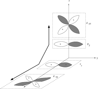
FIG. 3.: Hopping between different orbitals on next nearest neighboring (nnn) Ti ions when hopping between neighboring oxygen p orbitals is allowed. The hopping matrix element is the product of matrix elements to hop from a Ti ion in a $d_{yz}$ state to an O ion in a $p_{y}$ state, then to an adjacent O ion also in a $p_{y}$ state, and finally to a nnn Ti ion in a $d_{xy}$ state.

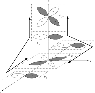
FIG. 4.: Hopping between different orbitals on nearest-neighboring Ti ions when hopping between neighboring oxygen p orbitals is allowed. The matrix elements for the two channels to hop from $d_{yz}$ to $d_{xy}$ have opposite signs, so that the total matrix element (summed over the two channels) is zero, as one would deduce from symmetry considerations. Thus the only processes involving two nearest neighboring oxygen ions are processes like those shown in Fig. 3 between nnn Ti ions.

The details of the mean-field treatment of this perturbation is given in Appendix D. Here we summarize the major analytic results obtained there for the wavevector-dependent spin susceptibility at the critical wavevector, ${\bf Q}$, $\chi_{\alpha\sigma;\beta\sigma^{\prime}}({\bf Q})=\chi_{\alpha\beta}({\bf Q})\delta_{\sigma,\sigma^{\prime}}$, where $\alpha$ and $\beta$ are orbital indices and $\sigma$ and $\sigma^{\prime}$ are spin indices. The result of Appendix D is that

$$\chi_{\alpha\beta}({\bf Q})^{-1} = \left[\begin{array}[]{c c c}12kT-8\epsilon&8\epsilon^{\prime}&8\epsilon^{\prime}\\ 8\epsilon^{\prime}&12kT-8\epsilon&8\epsilon^{\prime}\\ 8\epsilon^{\prime}&8\epsilon^{\prime}&12kT-8\epsilon\\ \end{array}\right].$$ (122)

The minimum eigenvalue is

$$\lambda = 12kT-8\epsilon-8\epsilon^{\prime}.$$ (123)

This gives

$$kT_{c} = 2(\epsilon+\epsilon^{\prime})/3.$$ (124)

By considering the eigenvectors and the effect of the fourth order terms, the analysis of Appendix D shows that nnn hopping does stabilize a ${\bf Q}$ antiferromagnetic structure, but the resulting 120^o state has zero net staggered spin. In addition, as before, there is a degeneracy between the spin-only states we have just described, and a state involving orbital order. As shown in III, fluctuations remove this degeneracy, so that we may consider only the mean-field solutions for spin-only states. Such a magnetic structure for which the local moment (summed over all flavors) vanishes, will be rather difficult to detect experimentally.

It is instructive to argue for the above results without actually performing the detailed calculations of Appendix D. We expect the effect of indirect exchange between nnn’s to induce an antiferromagnetic interaction between the spins of different orbital flavors of nnn’s. Note that the wavevector ${\bf Q}$ describes a two sub-lattice structure in which nnn’s are on the same sub-lattice. Accordingly, as far as mean-field theory is concerned, an nnn interaction between different flavors is equivalent to an antiferromagnetic interaction between spins of different flavors on the same site. So the spins of the three orbital flavors form the same structure as a triangular lattice antiferromagnet,[27] namely the spins of the three different orbital flavors are equal in magnitude and all lie in a single plane with orientations 120^o apart. This state still has global rotational invariance, but also, as does the triangular lattice antiferromagnet, it has degeneracy with respect to rotation of the spins of two flavors about the axis of the spin of the third flavor.

C Hund’s Rule Coupling

We now consider the effect of Hund’s rule coupling. Our aim is to see how this perturbation selects an ordered phase from among those phases which would first become critical in the absence of this perturbation as the temperature is reduced. To leading order in $\eta\equiv J_{H}/U$, where $J_{H}$ is the Hund’s rule coupling constant (which is positive in real systems), as discussed in Appendix E, this perturbation reads [28]

$$\delta{\cal H}_{KK} = \epsilon\eta\sum_{\langle ij\rangle}\sum_{\beta\gamma\neq\langle ij\rangle}\sum_{\sigma\sigma^{\prime}}\Bigl{(}c^{\dagger}_{i\gamma\sigma}c_{i\beta\sigma}c^{\dagger}_{j\gamma\sigma^{\prime}}c_{j\beta\sigma^{\prime}}$$ (125)

$$- c^{\dagger}_{i\gamma\sigma^{\prime}}c_{i\beta\sigma}c^{\dagger}_{j\gamma\sigma}c_{j\beta\sigma^{\prime}}+c^{\dagger}_{i\gamma\sigma}c_{i\beta\sigma}c^{\dagger}_{j\beta\sigma^{\prime}}c_{j\gamma\sigma^{\prime}}$$ (126)

$$- c^{\dagger}_{i\beta\sigma^{\prime}}c_{i\beta\sigma}c^{\dagger}_{j\gamma\sigma}c_{j\gamma\sigma^{\prime}}-2c^{\dagger}_{i\beta\sigma}c_{i\beta\sigma}c^{\dagger}_{j\gamma\sigma^{\prime}}c_{j\gamma\sigma^{\prime}}$$ (127)

$$+ 2c^{\dagger}_{i\gamma\sigma^{\prime}}c_{i\beta\sigma}c^{\dagger}_{j\beta\sigma}c_{j\gamma\sigma^{\prime}}\Bigr{)},$$ (128)

where $\epsilon=t^{2}/U$, as before. [29] To see the effect of this perturbation within mean-field theory, we calculate its average (see Appendix E for details). Confining to averages which are critical when $\eta=0$, (i.e., ${\mbox{\boldmath{$A$}}}_{\alpha\alpha}$ and $\vec{{\mbox{\boldmath{$B$}}}}_{\alpha\alpha}$), the result of Appendix E is

$$\langle\delta{\cal H}_{KK}\rangle = \epsilon\eta\sum_{\langle ij\rangle}\sum_{\beta\gamma\neq\langle ij\rangle}\Bigl{(}10{\mbox{\boldmath{$A$}}}_{\beta\beta}(i){\mbox{\boldmath{$A$}}}_{\beta\beta}(j)$$ (129)

$$- 10{\mbox{\boldmath{$A$}}}_{\beta\beta}(i){\mbox{\boldmath{$A$}}}_{\gamma\gamma}(j)+2\vec{{\mbox{\boldmath{$B$}}}}_{\beta\beta}(i)\cdot\vec{{\mbox{\boldmath{$B$}}}}_{\beta\beta}(j)$$ (130)

$$- 2\vec{{\mbox{\boldmath{$B$}}}}_{\beta\beta}(i)\cdot\vec{{\mbox{\boldmath{$B$}}}}_{\gamma\gamma}(j)\Bigr{)}.$$ (131)

Using Eqs. (11) and (89) to write the order parameters in terms of the $a_{\ell}$’s and the $s_{\alpha\gamma}$’s, this contributes a perturbation to the free energy given by

$$\delta F = \frac{1}{2}\sum_{k,l}\delta\left[{\mbox{\boldmath{$\chi$}}}_{n}^{-1}({\bf q})\right]_{kl}a_{k}({\bf q})a_{l}(-{\bf q})$$ (132)

$$+ \frac{1}{2}\sum_{\alpha\beta\gamma}\delta\left[{\mbox{\boldmath{$\chi$}}}_{s}^{-1}({\bf q})\right]_{\alpha\beta}^{\gamma}s_{\alpha\gamma}({\bf q})s_{\beta\gamma}(-{\bf q}),$$ (133)

where

$$\delta[{\mbox{\boldmath{$\chi$}}}_{n}^{-1}({\bf q})]$$ (134)

$$= -20\epsilon\eta\left[\begin{array}[]{cc}-\frac{1}{3}(2c_{x}+2c_{y}-c_{z})&\frac{1}{\sqrt{3}}(c_{x}-c_{y})\\ \frac{1}{\sqrt{3}}(c_{x}-c_{y})&-c_{z}\end{array}\right],$$ (137)

and

$$\delta[{\mbox{\boldmath{$\chi$}}}_{s}^{-1}({\bf q})] = -4\epsilon\eta\left[\begin{array}[]{ccc}0&c_{z}&c_{y}\\ c_{z}&0&c_{x}\\ c_{y}&c_{x}&0\end{array}\right].$$ (141)

If the minimum eigenvalue of $\delta{\mbox{\boldmath{$\chi$}}}^{-1}$ at wavevector ${\bf Q}$ is negative, then the instability temperature for the associated order parameter is raised by the perturbation and vice versa. Note that at wavevector ${\bf Q}$, $c_{x}=c_{y}=c_{z}=-1$ the eigenvalues of $\delta\left[{\mbox{\boldmath{$\chi$}}}_{s}^{-1}({\bf q})\right]$ are $8\eta\epsilon$, $-4\eta\epsilon$, and $-4\eta\epsilon$. On the other hand, the eigenvalues of $\delta\left[{\mbox{\boldmath{$\chi$}}}^{-1}_{n}({\bf q})\right]$ are both $-20\eta\epsilon$. From this result we conclude that Hund’s rule coupling favors antiferromagnetic orbital ordering, as described by the order parameters $a_{1}({\bf Q})$ and $a_{2}({\bf Q})$. Since the mean-field temperature for spin and orbital ordering were degenerate for $\eta=0$, we conclude that within mean-field theory the addition of an infinitesimal Hund’s rule coupling gives rise to an ordering transition in which the ordered state shows long-range antiferromagnetic orbital order, characterized by the order-parameters $a_{1}({\bf Q})$ and $a_{2}({\bf Q})$. However, since we have shown elsewhere[16] that for the bare KK model, fluctuations stabilize the spin-only states relative to orbital states, we conclude that when fluctuations are taken into account, it will take a finite amount of Hund’s rule coupling to bring about orbital ordering. For spin ordering the mean-field state is degenerate with respect to an arbitrary rotation. This is reflected by the fact that the term which is fourth order in the spin components is isotropic.

We now discuss the anisotropy in the mean-field solution for orbital order. We want to determine the form the free energy assumes in terms of the Fourier-transformed variables $a_{1}({\bf Q})$ and $a_{2}({\bf Q})$. Wavevector conservation dictates that we can have only products involving an even number of these variables. If we write $a_{1}({\bf Q})=a\cos\theta_{\bf Q}$ and $a_{2}({\bf Q})=a\sin\theta_{\bf Q}$, then we show in Appendix F that the contribution to the free energy of order $a^{4}$ is independent of $\theta_{\bf Q}$, but the term of order $a^{6}$ is of the form $\delta F=a^{6}[C_{0}+C_{6}\cos(6\theta_{\bf Q}+\phi)]$. This form indicates an anisotropy, so that the mean-field solution is not subject to a rotational degeneracy in $a_{1}$-$a_{2}$ space. If $C_{6}$ is positive and $\phi=0$, these minima come from the six angles that are equivalent to $\theta_{\bf Q}=\pi/2+n\pi/3$. For $\theta_{\bf Q}=\pi/2$, $a_{1}=0$ and we have ordering involving only $a_{2}$, so that $\langle N_{z}\rangle=1/3$, $\langle N_{x}\rangle=1/3+\sqrt{2}a_{2}(i)$ and $\langle N_{y}\rangle=1/3-\sqrt{2}a_{2}(i)$. The six minima of $\cos(6\theta_{\bf Q})$ correspond to the six permutations of coordinate labels which give equivalent ordering under cubic symmetry. Somewhat different states occur for $C_{6}$ negative, but different solutions reproduce the cubic symmetry operations.

D Spin-Orbit Interactions and Hund’s Rule Coupling

Here we briefly consider the case when we include the effects of both spin-orbit and Hund’s rule coupling. We consider the instabilities at wavevector ${\bf Q}$. In this case we construct the spin susceptibility ${\mbox{\boldmath{$\chi$}}}^{-1}_{s}({\bf Q})$ [defined as in Eq. (133)]. For the present case we may use our previous calculations in Eqs. (102) and (133) to write

$${\mbox{\boldmath{$\chi$}}}_{s}^{-1}(\gamma) = \left[\begin{array}[]{c c c}\lambda_{0}+x&y&y\\ y&\lambda_{0}+x&z\\ y&z&\lambda_{0}+x\\ \end{array}\right],$$ (145)

where the first row and column refer to $s_{\gamma\gamma}$ and the other two rows and columns refer to $s_{\beta\gamma}$ with $\beta\not=\gamma$ and

$$x=-\frac{4}{3}C_{0},\ \ y=\frac{4}{3}C_{0}+4\epsilon\eta,\ \ z=-\frac{4}{3}C_{0}+4\epsilon\eta.$$ (146)

Similarly the orbital susceptibility (also at wavevector ${\bf Q}$) is given by

$${\mbox{\boldmath{$\chi$}}}({\bf Q})^{-1}_{n} = \left[\begin{array}[]{c c}\lambda_{0}+w&0\\ 0&\lambda_{0}+w\\ \end{array}\right],$$ (149)

where

$$w = 2C_{0}-20\epsilon\eta\ .$$ (150)

In the above $C_{0}=4\lambda^{2}/\epsilon$ must be positive, $\lambda_{0}=12kT+8\epsilon$, and $\eta\equiv J_{H}/U$ is normally positive, although we may draw a phase diagram incorporating the possibility that $\eta$ is negative.

As we have seen, with only spin-orbit interactions we get a spin state which has a rotational degeneracy, and with only Hund’s rule interactions, the ordered phase has orbital rather than spin ordering. When both interactions are present, there is a competition between these two types of ordering. To study this competition we need to compare the minimum eigenvalue of the two susceptibility matrices given above. For the inverse spin susceptibility matrix $y\geq z$, in which case the minimum eigenvalue is

$$\lambda_{-} = \lambda_{0}+x+(z/2)-\sqrt{(z/2)^{2}+2y^{2}}\ .$$ (151)

On dimensional grounds, we expect that for $C_{0}<\tau\eta\epsilon$, where $\tau$ is a constant, Hund’s rule coupling will dominate and will lead to orbital ordering. Indeed after some algebra we find this condition with $\tau\approx 2.7$. This may be written as $\eta>0$ and $\lambda<\tau^{\prime}\epsilon\sqrt{\eta}$, where $\tau^{\prime}=\sqrt{\tau}/2\approx 0.82$

FIG. 5.: The mean-field phase diagram as a function of the spin-orbit coupling constant $\lambda$ and the Hund’s rule coupling constant $\eta\equiv J_{H}/U$ (which is normally positive). In the “spin-only” phase for $\eta\not=0$, the staggered moment orients along a $(1,1,1)$ direction, but the staggered spin moments of different orbital states are not collinear, thus reducing the net staggered spin. For $\eta=0$, the mean-field state has rotational degeneracy, so no easy direction of staggered magnetization is selected and the excitation spectrum is gapless. In the orbital phase one has the six-fold anisotropy associated with the equivalent choices for differently populating orbital levels in cubic symmetry, as is discussed in the text.

which gives rise to the phase diagram shown in Fig. 5. This phase diagram is not quite the same as that found in Ref. [28] for zero temperature. When we have spin ordering, we may analyze the fourth-order terms, as is done in Eq. (109). That analysis shows that unless the minimum eigenvector has components of equal magnitude, the anisotropy favors spin ordering along a $(1,1,1)$ direction. The condition that the eigenvector be $(-1,1,1)$ is that $y+z=0$. This can only happen when $\eta=0$. Then we have isotropy and the mean-field state exhibits rotational degeneracy. Otherwise, when $\eta\not=0$, the fourth-order terms give rise to an anisotropy that orients the staggered spin along a $(1,1,1)$ direction. We should also remind the reader that fluctuations favor the spin-only state, so that the phase boundary shown in Fig. 5 will be shifted by fluctuations to larger positive $\eta$. In the regime of orbital ordering, we indicate in Appendix F the existence of a six-fold anisotropy in the variables $a_{1}({\bf Q})$ and $a_{2}({\bf Q})$, such that the six equivalent minima correspond to the six possible states which are obtained by choosing $N_{\alpha}=1/3$ for one coordinate $\alpha$, and then occupying the two other orbitals with probability $1/3\pm\Delta$.

VI DISCUSSION AND SUMMARY

The cubic KK model has some very unusual and interesting symmetries which cause mean-field theory to have some unusual features. In particular, for the simplest KK Hamiltonian, we found that mean-field theory leads to criticality for the wavevector-dependent spin susceptibility associated with orbital $\alpha$ which is dispersionless along the $q_{\alpha}$ direction of wavevector. This result is consistent with the previous observation[14] that the Hamiltonian is invariant against an arbitrary rotation of the total spin in the orbital $\alpha$ summed over all spins in any single plane perpendicular to the $\alpha$ axis. This ‘soft mode’ behavior prevents the development of long-range spin order at any nonzero temperature,[14] even though the system is a three dimensional one.

Any perturbation which destroys this peculiar symmetry will enable the system to develop long-range spin order. In particular, we investigate the role of a) spin-orbit interactions, b) second-neighbor hopping, and c) Hund’s rule coupling in stabilizing long-range spin order. In the presence of spin-orbit interaction we find wavevector selection (because now the spin of different orbitals can not be freely rotated relative to one another) into a two-sublattice antiferromagnetic state with a greatly reduced spin magnitude. Since experiment shows such a reduction,[8] this mechanism may be operative to some extent. However, as noted previously,[14] the excitation spectrum does not have a gap until further perturbations are also included. The mean-field solution is consistent with this conclusion, because the mean-field state which minimizes the trial free energy is degenerate with respect to a global rotation of the staggered spin.

The ordered state which results when nnn hopping is added to the bare KK Hamiltonian is quite unusual. In this state, each orbital flavor has a staggered spin moment, but these three staggered spin moments form a 120^o degree state such that the total staggered spin moment (summed over the three orbital states) is zero! It is not immediately obvious how such long-range order would be observed. Finally, we show that when the bare KK Hamiltonian is perturbed by the addition of only Hund’s rule coupling, the resulting ordered state may exhibit long-range antiferromagnetic orbital order.

One caveat concerning our result should be mentioned. All our results are based on a stability analysis of the disordered phase. If the ordering transition is a discontinuous one, our results might not reveal such a transition. In III we will present results for the temperature-dependence of the various mean-field solutions. Further analysis of the ordered phase is needed to obtain a phase diagram at $T=0$, as is done in Ref.[28].

It should be emphasized again that all the results in this paper are based on the assumption that nearest-neighbor bonds along an axis $\alpha$ are ’inactive’, namely that there is no direct hopping between $\alpha$ orbitals along such bonds. Even within cubic symmetry, such hopping could still exist, alas with a very small hopping energy $t^{\prime\prime}$. However, as soon as we add such terms, the vertical bond in Fig. 1b becomes active, and Eqs. (45) and (47) have the additional contributions $\Delta\chi^{-1}_{\alpha\alpha}=2\epsilon^{\prime\prime}c_{\alpha}$ and $\Delta\chi^{-1}_{\alpha\beta}=2\epsilon^{\prime\prime}(c_{\alpha}+c_{\beta})$, with $\epsilon^{\prime\prime}=t^{\prime\prime 2}/U$. This introduces dispersion in all directions, and select order at $\vec{q}=\vec{Q}$. Distortions away from the cubic structure can enhace $t^{\prime\prime}$, and stabilize such order even further.

One general conclusion from our work is that it is not safe to associate properties of real experimental systems with properties of a model Hamiltonian unless one is absolutely sure that the real system is a realization (at least in all important aspects) of the model Hamiltonian. Here the ideal cubic KK Hamiltonian has properties which are quite different from those observed for systems it supposedly describes. What this means is that it will be necessary to take into account effects that one might have been tempted to ignore in order to identify a model that is truly appropriate for experimentally realizable systems. Alternatively, perhaps our work will inspire experimentalists to find systems that are as close as possible to that of the ideal cubic KK Hamiltonian treated here. Such systems would have quite striking and anomalous properties.

A Higher-order terms in the free-energy

Here we employ Eqs. (7), (8), and (9) in conjunction with Eq. (31), to derive general expressions for the cubic and quartic terms of the free energy.

The ‘bare’ cubic terms in the free-energy arise from Tr[$X^{3}$]. We find

$${\rm Tr}[X^{3}(i)]=\sum_{\alpha_{i}\beta_{i}}\sum_{\rho_{i}\eta_{i}}{\rm Tr}\Bigl{[}c^{\dagger}_{i\alpha_{1}\rho_{1}}Y_{\alpha_{1}\rho_{1}\beta_{1}\eta_{1}}(i)c_{i\beta_{1}\eta_{1}}c^{\dagger}_{i\alpha_{2}\rho_{2}}Y_{\alpha_{2}\rho_{2}\beta_{2}\eta_{2}}(i)c_{i\beta_{2}\eta_{2}}c^{\dagger}_{i\alpha_{3}\rho_{3}}Y_{\alpha_{3}\rho_{3}\beta_{3}\eta_{3}}(i)c_{i\beta_{3}\eta_{3}}\Bigr{]}$$ (A1)

$$= \sum_{\alpha_{i}\rho_{i}}\Bigl{[}{\mbox{\boldmath{$A$}}}_{\alpha_{1}\alpha_{2}}(i)\delta_{\rho_{1}\rho_{2}}+\vec{{\mbox{\boldmath{$B$}}}}_{\alpha_{1}\alpha_{2}}(i)\cdot\vec{{\mbox{\boldmath{$\sigma$}}}}_{\rho_{1}\rho_{2}}\Bigr{]}\Bigl{[}{\mbox{\boldmath{$A$}}}_{\alpha_{2}\alpha_{3}}(i)\delta_{\rho_{2}\rho_{3}}+\vec{{\mbox{\boldmath{$B$}}}}_{\alpha_{2}\alpha_{3}}(i)\cdot\vec{{\mbox{\boldmath{$\sigma$}}}}_{\rho_{2}\rho_{3}}\Bigr{]}\Bigl{[}{\mbox{\boldmath{$A$}}}_{\alpha_{3}\alpha_{1}}(i)\delta_{\rho_{3}\rho_{1}}+\vec{{\mbox{\boldmath{$B$}}}}_{\alpha_{3}\alpha_{1}}(i)\cdot\vec{{\mbox{\boldmath{$\sigma$}}}}_{\rho_{3}\rho_{1}}\Bigr{]}.$$ (A2)

Making use of the identity Eq. (30), this becomes

$${\rm Tr}[X^{3}(i)] = 2\sum_{\alpha_{i}}\Bigl{\{}{\mbox{\boldmath{$A$}}}_{\alpha_{1}\alpha_{2}}(i){\mbox{\boldmath{$A$}}}_{\alpha_{2}\alpha_{3}}(i){\mbox{\boldmath{$A$}}}_{\alpha_{3}\alpha_{1}}(i)+3{\mbox{\boldmath{$A$}}}_{\alpha_{1}\alpha_{2}}(i)\vec{{\mbox{\boldmath{$B$}}}}_{\alpha_{2}\alpha_{3}}(i)\cdot\vec{{\mbox{\boldmath{$B$}}}}_{\alpha_{3}\alpha_{1}}(i)$$ (A4)

$$\ \ \ \ \ \ \ \ +i(\vec{{\mbox{\boldmath{$B$}}}}_{\alpha_{1}\alpha_{2}}(i)\times\vec{{\mbox{\boldmath{$B$}}}}_{\alpha_{2}\alpha_{3}}(i))\cdot\vec{{\mbox{\boldmath{$B$}}}}_{\alpha_{3}\alpha_{1}}(i)\Bigr{\}}.$$

The ‘bare’ quartic terms in the free-energy arise from Tr[$X^{4}$]. We find

$${\rm Tr}[X^{4}(i)] = \sum_{\alpha_{i}\beta_{i}}\sum_{\rho_{i}\eta_{i}}{\rm Tr}\Bigl{[}c^{\dagger}_{i\alpha_{1}\rho_{1}}Y_{\alpha_{1}\rho_{1}\beta_{1}\eta_{1}}(i)c_{i\beta_{1}\eta_{1}}c^{\dagger}_{i\alpha_{2}\rho_{2}}Y_{\alpha_{2}\rho_{2}\beta_{2}\eta_{2}}(i)c_{i\beta_{2}\eta_{12}}$$ (A6)

$$\times c^{\dagger}_{i\alpha_{3}\rho_{3}}Y_{\alpha_{3}\rho_{3}\beta_{3}\eta_{3}}(i)c_{i\beta_{3}\eta_{3}}c^{\dagger}_{i\alpha_{4}\rho_{4}}Y_{\alpha_{4}\rho_{4}\beta_{4}\eta_{4}}(i)c_{i\beta_{4}\eta_{4}}\Bigr{]}$$

$$= \sum_{\alpha_{i}}\sum_{\rho_{i}}\Big{[}{\mbox{\boldmath{$A$}}}_{\alpha_{1}\alpha_{2}}(i)\delta_{\rho_{1}\rho_{2}}+\vec{{\mbox{\boldmath{$B$}}}}_{\alpha_{1}\alpha_{2}}(i)\cdot\vec{{\mbox{\boldmath{$\sigma$}}}}_{\rho_{1}\rho_{2}}\Bigr{]}\Bigl{[}{\mbox{\boldmath{$A$}}}_{\alpha_{2}\alpha_{3}}(i)\delta_{\rho_{2}\rho_{3}}+\vec{{\mbox{\boldmath{$B$}}}}_{\alpha_{2}\alpha_{3}}(i)\cdot\vec{{\mbox{\boldmath{$\sigma$}}}}_{\rho_{2}\rho_{3}}\Bigr{]}$$ (A8)

$$\times\Bigl{[}{\mbox{\boldmath{$A$}}}_{\alpha_{3}\alpha_{4}}(i)\delta_{\rho_{3}\rho_{4}}+\vec{{\mbox{\boldmath{$B$}}}}_{\alpha_{3}\alpha_{4}}(i)\cdot\vec{{\mbox{\boldmath{$\sigma$}}}}_{\rho_{3}\rho_{4}}\Bigr{]}\Bigl{[}{\mbox{\boldmath{$A$}}}_{\alpha_{24}\alpha_{1}}(i)\delta_{\rho_{4}\rho_{1}}+\vec{{\mbox{\boldmath{$B$}}}}_{\alpha_{4}\alpha_{1}}(i)\cdot\vec{{\mbox{\boldmath{$\sigma$}}}}_{\rho_{4}\rho_{1}}\Bigr{]}.$$

Again using the identity Eq. (30), this becomes

$${\rm Tr}[X^{4}(i)] = 2\sum_{\alpha_{i}}\Bigl{\{}\Bigl{(}{\mbox{\boldmath{$A$}}}_{\alpha_{1}\alpha_{2}}(i){\mbox{\boldmath{$A$}}}_{\alpha_{2}\alpha_{3}}(i)+\vec{{\mbox{\boldmath{$B$}}}}_{\alpha_{1}\alpha_{2}}(i)\cdot\vec{{\mbox{\boldmath{$B$}}}}_{\alpha_{2}\alpha_{3}}(i)\Bigr{)}\Bigl{(}{\mbox{\boldmath{$A$}}}_{\alpha_{3}\alpha_{4}}(i){\mbox{\boldmath{$A$}}}_{\alpha_{4}\alpha_{1}}(i)+\vec{{\mbox{\boldmath{$B$}}}}_{\alpha_{3}\alpha_{4}}(i)\cdot\vec{{\mbox{\boldmath{$B$}}}}_{\alpha_{4}\alpha_{1}}(i)\Bigr{)}$$ (A9)

$$+ \Bigl{(}{\mbox{\boldmath{$A$}}}_{\alpha_{1}\alpha_{2}}(i)\vec{{\mbox{\boldmath{$B$}}}}_{\alpha_{2}\alpha_{3}}(i)+\vec{{\mbox{\boldmath{$B$}}}}_{\alpha_{1}\alpha_{2}}(i){\mbox{\boldmath{$A$}}}_{\alpha_{2}\alpha_{3}}(i)+i\vec{{\mbox{\boldmath{$B$}}}}_{\alpha_{1}\alpha_{2}}(i)\times\vec{{\mbox{\boldmath{$B$}}}}_{\alpha_{2}\alpha_{3}}(i)\Bigr{)}$$ (A11)

$$\cdot\Bigl{(}{\mbox{\boldmath{$A$}}}_{\alpha_{3}\alpha_{4}}(i)\vec{{\mbox{\boldmath{$B$}}}}_{\alpha_{4}\alpha_{1}}(i)+\vec{{\mbox{\boldmath{$B$}}}}_{\alpha_{3}\alpha_{4}}(i){\mbox{\boldmath{$A$}}}_{\alpha_{4}\alpha_{1}}(i)+i\vec{{\mbox{\boldmath{$B$}}}}_{\alpha_{3}\alpha_{4}}(i)\times\vec{{\mbox{\boldmath{$B$}}}}_{\alpha_{4}\alpha_{1}}(i)\Bigr{)}\Bigr{\}}.$$

B CUBIC FREE-ENERGY TERMS

Referring to Eq. (A4), the relevant terms for our purpose come from the second and the third terms there. Working in Fourier space we hence have

$$\delta F = -\frac{8\epsilon}{\sqrt{N}}\sum_{{\bf q}_{1}{\bf q}_{2}}\sum_{\alpha_{1}\alpha_{2}\alpha_{3}}\Bigl{[}3{\mbox{\boldmath{$A$}}}_{\alpha_{1}\alpha_{2}}({\bf q}_{1})\vec{{\mbox{\boldmath{$B$}}}}_{\alpha_{2}\alpha_{3}}({\bf q}_{2})\cdot\vec{{\mbox{\boldmath{$B$}}}}_{\alpha_{3}\alpha_{1}}(-{\bf q}_{1}-{\bf q}_{2})$$ (B1)

$$+ i\vec{{\mbox{\boldmath{$B$}}}}_{\alpha_{1}\alpha_{2}}({\bf q}_{1})\times\vec{{\mbox{\boldmath{$B$}}}}_{\alpha_{2}\alpha_{3}}({\bf q}_{2})\cdot\vec{{\mbox{\boldmath{$B$}}}}_{\alpha_{3}\alpha_{1}}(-{\bf q}_{1}-{\bf q}_{2})\Bigr{]}.$$ (B2)

When one of the quantities $B$ here acts as the spatially uniform field [see Eq. (84)], this expression becomes

$$\delta F = -\frac{8\epsilon}{\sqrt{N}}\sum_{{\bf q}}\sum_{\alpha_{1}\alpha_{2}\alpha_{3}}\Bigl{[}3{\mbox{\boldmath{$A$}}}_{\alpha_{1}\alpha_{2}}({\bf q})\vec{{\mbox{\boldmath{$B$}}}}_{\alpha_{2}\alpha_{3}}\cdot\vec{{\mbox{\boldmath{$B$}}}}_{\alpha_{3}\alpha_{1}}(-{\bf q})+3{\mbox{\boldmath{$A$}}}_{\alpha_{1}\alpha_{2}}({\bf q})\vec{{\mbox{\boldmath{$B$}}}}_{\alpha_{2}\alpha_{3}}(-{\bf q})\cdot\vec{{\mbox{\boldmath{$B$}}}}_{\alpha_{3}\alpha_{1}}$$ (B3)

$$+ i\vec{{\mbox{\boldmath{$B$}}}}_{\alpha_{1}\alpha_{2}}\times\vec{{\mbox{\boldmath{$B$}}}}_{\alpha_{2}\alpha_{3}}({\bf q})\cdot\vec{{\mbox{\boldmath{$B$}}}}_{\alpha_{3}\alpha_{1}}(-{\bf q})+i\vec{{\mbox{\boldmath{$B$}}}}_{\alpha_{1}\alpha_{2}}({\bf q})\times\vec{{\mbox{\boldmath{$B$}}}}_{\alpha_{2}\alpha_{3}}\cdot\vec{{\mbox{\boldmath{$B$}}}}_{\alpha_{3}\alpha_{1}}(-{\bf q})$$ (B4)

$$+ i\vec{{\mbox{\boldmath{$B$}}}}_{\alpha_{1}\alpha_{2}}({\bf q})\times\vec{{\mbox{\boldmath{$B$}}}}_{\alpha_{2}\alpha_{3}}(-{\bf q})\cdot\vec{{\mbox{\boldmath{$B$}}}}_{\alpha_{3}\alpha_{1}}\Bigr{]},$$ (B5)

where $\vec{{\mbox{\boldmath{$B$}}}}$ which does not depend on ${\bf q}$ is the uniform field.

We first consider the terms involving the $A$’s. The relevant contributions come from $\alpha_{3}=\alpha_{1}$ [the first term in Eq. (B5))] and $\alpha_{3}=\alpha_{2}$ [the second term there]. Hence we find

$$\delta F_{A} = -\frac{24\epsilon}{\sqrt{N}}\sum_{\bf q}{\sum_{\alpha\beta}}^{\prime}{\mbox{\boldmath{$A$}}}_{\alpha\beta}({\bf q})\vec{{\mbox{\boldmath{$B$}}}}_{\beta\alpha}\cdot\Bigl{(}\vec{{\mbox{\boldmath{$B$}}}}_{\alpha\alpha}(-{\bf q})+\vec{{\mbox{\boldmath{$B$}}}}_{\beta\beta}(-{\bf q})\Bigr{)},$$ (B6)

where $\sum^{\prime}_{\alpha\beta}$ denotes that $\alpha\neq\beta$. When we minimize $F_{2}+\delta F_{A}$ with respect to ${\mbox{\boldmath{$A$}}}_{\alpha\beta}({\bf q})$, and use Eqs. (47) and (84), we get the contribution

$$\delta F_{A} = -72g_{0}^{2}\epsilon\sum_{\bf q}\sum_{\alpha\beta\gamma}\epsilon_{\alpha\beta\gamma}^{2}[s_{\alpha\gamma}({\bf q})+s_{\beta\gamma}({\bf q})][s_{\alpha\gamma}(-{\bf q})+s_{\beta\gamma}(-{\bf q})][2+\cos(q_{\gamma}a)]^{-1},$$ (B7)

where we have defined

$$s_{\alpha\gamma}({\bf q})\equiv{\mbox{\boldmath{$B$}}}^{\gamma}_{\alpha\alpha}({\bf q}).$$ (B8)

Also, since we are interested in the free energy to quadratic order in the order parameters, we have set $kT=2\epsilon/3$.

In this result we want to keep only contributions which involve the critical variables. For $s_{\alpha\gamma}({\bf q})$ this means that we sum over ${\bf q}$’s such that $q_{\beta}=\pi/a$, for $\beta\not=\alpha$. Thus for each $s_{\alpha\gamma}$ the wavevector sum is a sum over the component $q_{\alpha}$, with the other components of ${\bf q}$ equal to $\pi/a$. We denote this type of sum by $\sum_{q_{\alpha}}$. Furthermore for a term involving components $s_{\alpha\gamma}$ and $s_{\beta\gamma}$ with different orbitals $\alpha$ and $\beta$, this sum reduces to the single wavevector ${\bf Q}=(\pi,\pi,\pi)/a$. So

$$\delta F_{A} = -144g_{0}^{2}\epsilon\sum_{\alpha\beta\gamma}\epsilon_{\alpha\beta\gamma}^{2}\Bigl{\{}\sum_{q_{\alpha}}{s_{\alpha\gamma}({\bf q})s_{\alpha\gamma}(-{\bf q})\over 2+\cos(q_{\gamma}a)}+s_{\alpha\gamma}({\bf Q})s_{\beta\gamma}({\bf Q})\Bigr{\}}.$$ (B9)

Here we will set $[2+\cos(q_{\gamma}a)]=1$ because for $s_{\alpha\gamma}$ (with $\alpha\not=\gamma$) we must have $q_{\gamma}=\pi/a$. This term favors ordering at wavevector ${\bf Q}$ with ${\bf s}_{\alpha}({\bf Q})$ collinear with $s_{\beta}({\bf Q})$, where ${\bf s}_{\alpha}({\bf Q})$ is a vector with components $[s_{\alpha x}({\bf Q})\ ,s_{\alpha y}({\bf Q})\ ,s_{\alpha z}({\bf Q})]$.

Next we consider the contribution coming from the terms with three $B$’s in Eq. (B5). Here we put one of the ${\bf q}$-dependent $B$’s to be diagonal in the orbital indices, to obtain

$$\delta F_{B} = -i\frac{36kT}{\sqrt{N}}\sum_{\bf q}{\sum_{\alpha\beta}}^{\prime}\sum_{\alpha_{1}\beta_{1}\gamma}\epsilon_{\alpha_{1}\beta_{1}\gamma}{\mbox{\boldmath{$B$}}}_{\alpha\beta}^{\gamma}({\bf q})({\mbox{\boldmath{$B$}}}_{\alpha\alpha}^{\beta_{1}}(-{\bf q})-{\mbox{\boldmath{$B$}}}_{\beta\beta}^{\beta_{1}}(-{\bf q})){\mbox{\boldmath{$B$}}}_{\beta\alpha}^{\alpha_{1}}.$$ (B10)

Eliminating the noncritical ${\mbox{\boldmath{$B$}}}_{\alpha\beta}^{\gamma}({\bf q})$ variables by minimizing $F_{2}+\delta F_{B}$ with respect to them, we get

$$\delta F_{B} = -1296(g_{0}kT)^{2}{\sum_{\alpha\beta}}^{\prime}\sum_{\bf q}\chi_{\alpha\beta}({\bf q})[s_{\beta\beta}({\bf q})-s_{\alpha\beta}({\bf q})][(s_{\beta\beta}(-{\bf q})-s_{\alpha\beta}(-{\bf q})],$$ (B11)

where $\chi$ is given in Eq. (47), and we have used the definition (B8). As before we set $kT=2\epsilon/3$ and separate the sums to be only over critical wavevectors for each orbital spin vector, in which case we have

$$\delta F_{B}=-144g_{0}^{2}\epsilon\sum_{\alpha\beta\gamma}\epsilon_{\alpha\beta\gamma}^{2}\Bigl{\{}\sum_{q_{\alpha}}[s_{\alpha\alpha}({\bf q})s_{\alpha\alpha}(-{\bf q})+s_{\alpha\beta}({\bf q})s_{\alpha\beta}(-{\bf q})]-2s_{\alpha\alpha}({\bf Q})s_{\beta\alpha}({\bf Q})\Bigr{\}}\ .$$ (B12)

Here we noted that $\chi_{\alpha\beta}({\bf q})=\chi_{\alpha\beta}({\bf Q})=1/(4\epsilon)$ because this component of $\chi$ depends on $q_{\gamma}$ which is always $\pi/a$ in the summation over wavevector.

In summary the total contribution to the quadratic free energy at order $\lambda^{2}$ is

$$F_{2}^{(3)}=\delta F_{A}+\delta F_{B} = -C_{0}\sum_{\alpha\beta\gamma}\epsilon_{\alpha\beta\gamma}^{2}\Bigl{\{}\Bigl{(}s_{\alpha\gamma}({\bf Q})s_{\beta\gamma}({\bf Q})-2s_{\beta\beta}({\bf Q})s_{\alpha\beta}({\bf Q})\Bigr{)}$$ (B13)

$$+ \sum_{q_{\alpha}}\Bigl{(}s_{\alpha\gamma}({\bf q})s_{\alpha\gamma}(-{\bf q})+s_{\alpha\alpha}({\bf q})s_{\alpha\alpha}(-{\bf q})+s_{\alpha\beta}({\bf q})s_{\alpha\beta}(-{\bf q})]\Bigr{)}\Bigr{\}},$$ (B14)

where we set $kT=2\epsilon/3$ and $C_{0}=144g_{0}^{2}\epsilon$.

C QUARTIC TERMS IN THE FREE ENERGY

Now we look at fourth order terms. These involve two critical order parameters and two powers of $\lambda$. Therefore, we pick from Eq. (A11) all terms involving at least two powers of $B$. Since two of the factors $B$ in each term have to be $\vec{{\mbox{\boldmath{$B$}}}}_{\alpha\beta}=-\vec{{\mbox{\boldmath{$B$}}}}_{\beta\alpha}$, with $\alpha\neq\beta$, [see Eq. (84)], we see that the terms involving a single power of $A$ vanish. Thus we have to consider the expression

$$36kT\sum_{i}\sum_{\stackrel{{\scriptstyle\alpha_{1}\alpha_{2}}}{{\alpha_{3}\alpha_{4}}}}\Bigl{(}4{\mbox{\boldmath{$A$}}}_{\alpha_{1}\alpha_{2}}{\mbox{\boldmath{$A$}}}_{\alpha_{2}\alpha_{3}}\vec{{\mbox{\boldmath{$B$}}}}_{\alpha_{3}\alpha_{4}}\cdot\vec{{\mbox{\boldmath{$B$}}}}_{\alpha_{4}\alpha_{1}}+2{\mbox{\boldmath{$A$}}}_{\alpha_{1}\alpha_{2}}{\mbox{\boldmath{$A$}}}_{\alpha_{3}\alpha_{4}}\vec{{\mbox{\boldmath{$B$}}}}_{\alpha_{2}\alpha_{3}}\cdot\vec{{\mbox{\boldmath{$B$}}}}_{\alpha_{4}\alpha_{1}}$$ (C1)

$$+ (\vec{{\mbox{\boldmath{$B$}}}}_{\alpha_{1}\alpha_{2}}\cdot\vec{{\mbox{\boldmath{$B$}}}}_{\alpha_{2}\alpha_{3}})(\vec{{\mbox{\boldmath{$B$}}}}_{\alpha_{3}\alpha_{4}}\cdot\vec{{\mbox{\boldmath{$B$}}}}_{\alpha_{4}\alpha_{1}})-(\vec{{\mbox{\boldmath{$B$}}}}_{\alpha_{1}\alpha_{2}}\times\vec{{\mbox{\boldmath{$B$}}}}_{\alpha_{2}\alpha_{3}})\cdot(\vec{{\mbox{\boldmath{$B$}}}}_{\alpha_{3}\alpha_{4}}\times\vec{{\mbox{\boldmath{$B$}}}}_{\alpha_{4}\alpha_{1}})\Bigr{)},$$ (C2)

where $A$ and $B$ are functions of the site index $i$. The first two members of Eq. (C2) are calculated for the case in which the $A$’s are critical, and the $B$’s are given by Eq. (84). Denoting their contribution to the self-energy by $\delta F_{2}^{(1)}$, we find

$$\delta F_{2}^{(1)} = 36kT\sum_{i}\sum_{\alpha\beta}\Bigl{(}4{\mbox{\boldmath{$A$}}}_{\alpha\alpha}^{2}(i)+2{\mbox{\boldmath{$A$}}}_{\alpha\alpha}(i){\mbox{\boldmath{$A$}}}_{\beta\beta}(i)\Bigr{)}\vec{{\mbox{\boldmath{$B$}}}}_{\alpha\beta}\cdot\vec{{\mbox{\boldmath{$B$}}}}_{\beta\alpha}$$ (C3)

$$= 36kTg_{0}^{2}\sum_{\alpha\beta\gamma}\epsilon^{2}_{\alpha\beta\gamma}\Bigl{(}(4{\mbox{\boldmath{$A$}}}_{\alpha\alpha}^{2}(i)+2{\mbox{\boldmath{$A$}}}_{\alpha\alpha}(i){\mbox{\boldmath{$A$}}}_{\beta\beta}(i)\Bigr{)}=216kTg_{0}^{2}\sum_{i}(a_{1}^{2}(i)+a_{2}^{2}(i)),$$ (C4)

where in the last step we have used Eq. (11).

The contribution of the remaining two members of Eq. (C2) is denoted $\delta F_{2}^{(2)}$. Here we have to take two of the $B$’s as critical, while the other two are given by Eq. (84). To shorten notations, we denote here the critical $B$ as ${\mbox{\boldmath{$B$}}}(i)$, while the non-critical one is simply written as $B$. We have

$$\delta F_{2}^{(2)}=72kT\sum_{i}\sum_{\alpha\beta}\Bigr{[}(\vec{{\mbox{\boldmath{$B$}}}}_{\alpha\alpha}(i)\cdot\vec{{\mbox{\boldmath{$B$}}}}_{\alpha\alpha}(i))(\vec{{\mbox{\boldmath{$B$}}}}_{\alpha\beta}\cdot\vec{{\mbox{\boldmath{$B$}}}}_{\beta\alpha})+(\vec{{\mbox{\boldmath{$B$}}}}_{\alpha\alpha}(i)\cdot\vec{{\mbox{\boldmath{$B$}}}}_{\alpha\beta})(\vec{{\mbox{\boldmath{$B$}}}}_{\alpha\alpha}(i)\cdot\vec{{\mbox{\boldmath{$B$}}}}_{\beta\alpha})$$ (C5)

$$+ (\vec{{\mbox{\boldmath{$B$}}}}_{\alpha\alpha}(i)\cdot\vec{{\mbox{\boldmath{$B$}}}}_{\alpha\beta})(\vec{{\mbox{\boldmath{$B$}}}}_{\beta\beta}(i)\cdot\vec{{\mbox{\boldmath{$B$}}}}_{\beta\alpha})-(\vec{{\mbox{\boldmath{$B$}}}}_{\alpha\alpha}(i)\times\vec{{\mbox{\boldmath{$B$}}}}_{\alpha\beta})\cdot(\vec{{\mbox{\boldmath{$B$}}}}_{\beta\beta}(i)\times\vec{{\mbox{\boldmath{$B$}}}}_{\beta\alpha})+(\vec{{\mbox{\boldmath{$B$}}}}_{\alpha\alpha}(i)\times\vec{{\mbox{\boldmath{$B$}}}}_{\alpha\beta})\cdot(\vec{{\mbox{\boldmath{$B$}}}}_{\alpha\alpha}(i)\times\vec{{\mbox{\boldmath{$B$}}}}_{\beta\alpha})\Bigr{]}.$$ (C6)

Making again use of Eq. (84), this expression becomes

$$\delta F_{2}^{(2)} = 72kTg_{0}^{2}\sum_{i}\sum_{\alpha\beta\gamma}\epsilon^{2}_{\alpha\beta\gamma}\Bigl{[}2\sum_{\nu}{\mbox{\boldmath{$B$}}}_{\alpha\alpha}^{\nu}(i){\mbox{\boldmath{$B$}}}_{\alpha\alpha}^{\nu}(i)-\sum_{\nu}{\mbox{\boldmath{$B$}}}_{\alpha\alpha}^{\nu}(i){\mbox{\boldmath{$B$}}}_{\beta\beta}^{\nu}(i)+2{\mbox{\boldmath{$B$}}}_{\alpha\alpha}^{\gamma}(i){\mbox{\boldmath{$B$}}}_{\beta\beta}^{\gamma}(i)\Bigr{]}.$$ (C7)

Transforming to Fourier space, noting that only the first term here contains ${\bf q}$ while in the other two we must necessarily have ${\bf q}={\bf Q}$, (because they involve simultaneous criticality of two flavors), we obtain

$$\delta F_{2}^{(2)} = 72kTg_{0}^{2}\Bigl{[}2\sum_{\bf q}\sum_{\alpha\beta}s_{\alpha\beta}({\bf q})s_{\alpha\beta}(-{\bf q})+\sum_{\alpha\beta\gamma}\epsilon^{2}_{\alpha\beta\gamma}\Bigl{(}2s_{\alpha\gamma}({\bf Q})s_{\beta\gamma}({\bf Q})-\sum_{\nu}s_{\alpha\nu}({\bf Q})s_{\beta\nu}({\bf Q})\Bigr{)}\Bigr{]},$$ (C8)

where we have used the definition Eq. (B8). The total contribution to the free energy from quartic terms is then

$$F_{2}^{(4)}=\delta F_{2}^{(1)}+\delta F_{2}^{(2)}.$$ (C9)

D MEAN-FIELD THEORY FOR nnn HOPPING

Starting from Eq. (115), we may write the perturbation due to next-nearest-neighbors in the form

$$V_{KK} = \epsilon^{\prime}\sum_{ij}\sum_{\alpha\beta\delta}\gamma_{\alpha}(i,j)\sum_{\rho\eta}\epsilon^{2}_{\alpha\beta\delta}\Bigl{[}c^{\dagger}_{i\beta\rho}c_{i\delta\eta}c^{\dagger}_{j\beta\eta}c_{j\delta\rho}+c^{\dagger}_{i\beta\rho}c_{i\beta\eta}c^{\dagger}_{j\delta\eta}c_{j\delta\rho}\Bigr{]}.$$ (D1)

Within our mean-field theory, the averages are taken separately on the operators belonging to the site $i$, and those belonging to site $j$. The required averages are then given in Eq. (26). The following contribution to the trial energy $U$ is then

$$\langle V_{KK}\rangle = 2\epsilon^{\prime}\sum_{ij}\sum_{\alpha\beta\delta}\gamma_{\alpha}(i,j)\epsilon^{2}_{\alpha\beta\delta}\Bigl{[}{\mbox{\boldmath{$A$}}}_{\delta\beta}(i){\mbox{\boldmath{$A$}}}_{\delta\beta}(j)+\vec{{\mbox{\boldmath{$B$}}}}_{\delta\beta}(i)\cdot\vec{{\mbox{\boldmath{$B$}}}}_{\delta\beta}(j)+{\mbox{\boldmath{$A$}}}_{\beta\beta}(i){\mbox{\boldmath{$A$}}}_{\delta\delta}(j)+\vec{{\mbox{\boldmath{$B$}}}}_{\beta\beta}(i)\cdot\vec{{\mbox{\boldmath{$B$}}}}_{\delta\delta}(j)\Bigr{]}.$$ (D2)

Transforming to Fourier space, noting that each site has four next-nearest neighbors in each $\alpha$-plane, we obtain

$$\langle V_{KK}\rangle = 8\epsilon^{\prime}\sum_{\bf q}\sum_{\alpha\beta\delta}\epsilon^{2}_{\alpha\beta\delta}c_{\beta}c_{\delta}\Bigl{[}{\mbox{\boldmath{$A$}}}_{\delta\beta}({\bf q}){\mbox{\boldmath{$A$}}}_{\delta\beta}(-{\bf q})+\vec{{\mbox{\boldmath{$B$}}}}_{\delta\beta}({\bf q})\cdot\vec{{\mbox{\boldmath{$B$}}}}_{\delta\beta}(-{\bf q})+{\mbox{\boldmath{$A$}}}_{\beta\beta}({\bf q}){\mbox{\boldmath{$A$}}}_{\delta\delta}(-{\bf q})+\vec{{\mbox{\boldmath{$B$}}}}_{\beta\beta}({\bf q})\cdot\vec{{\mbox{\boldmath{$B$}}}}_{\delta\delta}(-{\bf q})\Bigr{]},$$ (D3)

where $c_{\beta}=\cos(q_{\beta}q)$. The result Eq. (D3) is now added to Eq. (41), in order to obtain the modifications in the susceptibility tensor. Specifying to the diagonal order-parameters ${\mbox{\boldmath{$A$}}}_{\alpha\alpha}$ and $\vec{{\mbox{\boldmath{$B$}}}}_{\alpha\alpha}$, the susceptibility tensor becomes [see Eq. (45)]

$${\mbox{\boldmath{$\chi$}}}({\bf q})^{-1} = \left[\begin{array}[]{c c c}12kT+4\epsilon(c_{y}+c_{z})&8\epsilon^{\prime}c_{x}c_{y}&8\epsilon^{\prime}c_{x}c_{z}\\ 8\epsilon^{\prime}c_{x}c_{y}&12kT+4\epsilon(c_{x}+c_{z})&8\epsilon^{\prime}c_{y}c_{z}\\ 8\epsilon^{\prime}c_{x}c_{z}&8\epsilon^{\prime}c_{y}c_{z}&12kT+4\epsilon(c_{x}+c_{y})\\ \end{array}\right].$$ (D7)

Now we look at the most critical wavevector, which here is ${\bf Q}$. There we have

$${\mbox{\boldmath{$\chi$}}}({\bf Q})^{-1} = \left[\begin{array}[]{c c c}12kT-8\epsilon&8\epsilon^{\prime}&8\epsilon^{\prime}\\ 8\epsilon^{\prime}&12kT-8\epsilon&8\epsilon^{\prime}\\ 8\epsilon^{\prime}&8\epsilon^{\prime}&12kT-8\epsilon\\ \end{array}\right].$$ (D11)

We begin with the analysis of the susceptibility tensor of the spin order parameters, which are given by the elements of ${\mbox{\boldmath{$B$}}}_{\alpha\alpha}$. Then we can use the matrix (D11). The minimum eigenvalue is

$$\lambda = 12kT-8\epsilon-8\epsilon^{\prime},$$ (D12)

which gives

$$kT_{c} = 2\epsilon/3+2\epsilon^{\prime}/3.$$ (D13)

Correspondingly, there are two degenerate eigenvectors:

$$|1\rangle = (0,1,-1)/\sqrt{2}\ ,\ \ |2\rangle=(2,-1,-1)/\sqrt{6}\ .$$ (D14)

To avoid confusion between orbital and spin labels, we will here denote the orbital states $x$, $y$, and $z$ by $a$, $b$, and $c$. Then in terms of normal mode vector $\xi$ and $\rho$ we have the orbital spin vectors as

$${\bf s}_{a}=-\frac{2}{\sqrt{6}}{\mbox{\boldmath{$\rho$}}}\ ,\ \ {\bf s}_{b}=\frac{1}{\sqrt{6}}{\mbox{\boldmath{$\rho$}}}+\frac{1}{\sqrt{2}}{\mbox{\boldmath{$\xi$}}}\ ,\ \ {\bf s}_{c}=\frac{1}{\sqrt{6}}{\mbox{\boldmath{$\rho$}}}-\frac{1}{\sqrt{2}}{\mbox{\boldmath{$\xi$}}}\ ,$$ (D15)

with

$${\bf s}_{a}^{2} = \frac{2}{3}{\mbox{\boldmath{$\rho$}}}^{2}\ ,\ \ {\bf s}_{b}^{2}={1\over 2}{\mbox{\boldmath{$\xi$}}}^{2}+{1\over 6}{\mbox{\boldmath{$\rho$}}}^{2}+\frac{1}{\sqrt{3}}{\mbox{\boldmath{$\xi$}}}\cdot{\mbox{\boldmath{$\rho$}}}\ ,\ \ {\bf s}_{c}^{2}={1\over 2}{\mbox{\boldmath{$\xi$}}}^{2}+{1\over 6}{\mbox{\boldmath{$\rho$}}}^{2}-\frac{1}{\sqrt{3}}{\mbox{\boldmath{$\xi$}}}\cdot{\mbox{\boldmath{$\rho$}}}\ .$$ (D16)

Evaluating the fourth-order free energy [see Eq. (79)] relevant to the spin-order parameters, we find

$$\Bigl{(}\sum_{\mu}{\bf s}_{\mu}^{2}\Bigr{)}^{2}-\sum_{\mu<\nu}{\bf s}_{\mu}^{2}{\bf s}_{\nu}^{2}=\frac{3}{4}({\mbox{\boldmath{$\xi$}}}^{2}+{\mbox{\boldmath{$\rho$}}}^{2})^{2}-\frac{1}{3}({\mbox{\boldmath{$\xi$}}}\times{\mbox{\boldmath{$\rho$}}})^{2}.$$ (D17)

What we see is that the fourth-order term does not select a particular direction for order. We have three angles which describe the degenerate manifold. For a given value of ${\mbox{\boldmath{$\xi$}}}^{2}+{\mbox{\boldmath{$\rho$}}}^{2}$, we optimize the term $({\mbox{\boldmath{$\xi$}}}\times{\mbox{\boldmath{$\rho$}}})^{2}$ by taking $|{\mbox{\boldmath{$\xi$}}}|=|{\mbox{\boldmath{$\rho$}}}|$ and making $\xi$ perpendicular to $\rho$. So, it takes two angles to specify $\xi$ (given that its length is fixed) and then we have one angle to specify $\rho$, given that $|{\mbox{\boldmath{$\rho$}}}|=|{\mbox{\boldmath{$\xi$}}}|$ and it is perpendicular to $\xi$. We now discuss what this choice of order parameters means for the spin vectors. First note that

$${\bf s}_{\alpha}^{2} = {\bf s}_{\beta}^{2}={\bf s}_{\gamma}^{2}=2{\mbox{\boldmath{$\xi$}}}^{2}/3\ .$$ (D18)

Also we see that the three orbital spin vectors obey

$${\bf s}_{a}\cdot{\bf s}_{b} = {\bf s}_{a}\cdot{\bf s}_{c}={\bf s}_{b}\cdot{\bf s}_{c}=-{\mbox{\boldmath{$\xi$}}}^{2}/3\ .$$ (D19)

The three vectors each make a 120^o angle with each other and must therefore lie in a single plane. We can fix, say, ${\bf s}_{\alpha}$. This accounts for two angles. Then the other two spin vectors require another angle to tell which plane they lie in. Note that there is zero net staggered moment. There is long-range spin order, but not of any simple type.

Next we analyze the susceptibility tensor of the occupation order parameters, which are given by the elements of ${\mbox{\boldmath{$A$}}}_{\alpha\alpha}$. Since the matrix ${\mbox{\boldmath{$A$}}}_{\alpha\alpha}$ is traceless, we use the parametrization Eq. (11) to obtain from Eq. (D11) the 2$\times$2 matrix

$$\chi_{\mu\nu}({\bf q})^{-1}=\left[\begin{array}[]{cc}12kT+\frac{2\epsilon}{3}(5c_{x}+5c_{y}+2c_{z})+\frac{8\epsilon^{\prime}}{3}(c_{x}c_{y}-2c_{y}c_{z}-2c_{z}c_{x})&\frac{2\epsilon}{\sqrt{3}}(c_{y}-c_{x})+\frac{8\epsilon^{\prime}}{\sqrt{3}}c_{z}(c_{y}-c_{x})\\ \frac{2\epsilon}{\sqrt{3}}(c_{y}-c_{x})+\frac{8\epsilon^{\prime}}{\sqrt{3}}c_{z}(c_{y}-c_{x})&12kT+2\epsilon(c_{x}+c_{y}+2c_{z})-8\epsilon^{\prime}c_{x}c_{y}\end{array}\right].$$ (D22)

This gives a minimum eigenvalue identical to that of Eq. (D12), which yields the same instability temperature as for the spin-only states. However, in the absence of second-neighbor coupling, the spin-only states are favored by fluctuations, [16] so that choice should be maintained for infinitesimal next-nearest neighbor hopping. (The situation could change when the next-nearest neighbor hopping exceed some threshold value.)

E Derivation of the Hund’s rule Hamiltonian

The Coulomb exchange terms for the $t_{2g}$-states can be written in the form [28]

$${\cal H}_{cex}=\frac{J_{H}}{2}\sum_{i}\sum_{\stackrel{{\scriptstyle\alpha\beta}}{{\alpha\neq\beta}}}\sum_{\sigma\sigma^{\prime}}\Bigl{(}c_{i\alpha\sigma}^{\dagger}c_{i\alpha\sigma^{\prime}}^{\dagger}c_{i\beta\sigma^{\prime}}c_{i\beta\sigma}+c_{i\alpha\sigma}^{\dagger}c_{i\beta\sigma^{\prime}}^{\dagger}c_{i\alpha\sigma^{\prime}}c_{i\beta\sigma}-2c_{i\alpha\sigma}^{\dagger}c_{i\beta\sigma^{\prime}}^{\dagger}c_{i\beta\sigma^{\prime}}c_{i\alpha\sigma}\Bigr{)},$$ (E1)

where $J_{H}$ is the Hund’s rule coupling. Adding ${\cal H}_{cex}$ to the Hamiltonian Eq. (2), the perturbation expansion in power of the transfer integrals $t$ now contains a term of the order $t^{2}J_{H}/U^{2}$, which reads

$$\delta{\cal H}_{KK} = \frac{t^{2}J_{H}}{U^{2}}\sum_{\langle ij\rangle}\sum_{\beta\gamma\neq\langle ij\rangle}\sum_{\sigma\sigma^{\prime}}\Bigl{(}c^{\dagger}_{i\gamma\sigma}c_{i\beta\sigma}c^{\dagger}_{j\gamma\sigma^{\prime}}c_{j\beta\sigma^{\prime}}-c^{\dagger}_{i\gamma\sigma^{\prime}}c_{i\beta\sigma}c^{\dagger}_{j\gamma\sigma}c_{j\beta\sigma^{\prime}}+c^{\dagger}_{i\gamma\sigma}c_{i\beta\sigma}c^{\dagger}_{j\beta\sigma^{\prime}}c_{j\gamma\sigma^{\prime}}$$ (E2)

$$- c^{\dagger}_{i\beta\sigma^{\prime}}c_{i\beta\sigma}c^{\dagger}_{j\gamma\sigma}c_{j\gamma\sigma^{\prime}}-2c^{\dagger}_{i\beta\sigma}c_{i\beta\sigma}c^{\dagger}_{j\gamma\sigma^{\prime}}c_{j\gamma\sigma^{\prime}}+2c^{\dagger}_{i\gamma\sigma^{\prime}}c_{i\beta\sigma}c^{\dagger}_{j\beta\sigma}c_{j\gamma\sigma^{\prime}}\Bigr{)}.$$ (E3)

Taking the thermal averages using Eq. (26) we find

$$\langle\delta{\cal H}_{KK}\rangle = \frac{t^{2}J_{H}}{U^{2}}\sum_{\langle ij\rangle}\sum_{\beta\gamma\neq\langle ij\rangle}\Bigl{(}2{\mbox{\boldmath{$A$}}}_{\beta\gamma}(i){\mbox{\boldmath{$A$}}}_{\beta\gamma}(j)+8{\mbox{\boldmath{$A$}}}_{\beta\gamma}(i){\mbox{\boldmath{$A$}}}_{\gamma\beta}(j)-10{\mbox{\boldmath{$A$}}}_{\beta\beta}(i){\mbox{\boldmath{$A$}}}_{\gamma\gamma}(j)$$ (E4)

$$- 2\vec{{\mbox{\boldmath{$B$}}}}_{\beta\gamma}(i)\cdot\vec{{\mbox{\boldmath{$B$}}}}_{\beta\gamma}(j)+4\vec{{\mbox{\boldmath{$B$}}}}_{\beta\gamma}(i)\cdot\vec{{\mbox{\boldmath{$B$}}}}_{\gamma\beta}(j)-2\vec{{\mbox{\boldmath{$B$}}}}_{\beta\beta}(i)\cdot\vec{{\mbox{\boldmath{$B$}}}}_{\gamma\gamma}(j)\Bigr{)}.$$ (E5)

where terms independent of the order-parameters were omitted.

F SIXTH-ORDER ANISOTROPY in the orbital sector

At fourth-order, the terms in $a_{1}(i)$ and $a_{2}(i)$ are proportional to $[a^{2}_{1}(i)+a_{2}^{2}(i)]^{2}$ [see Eq. (79)], and there is complete isotropy in $a_{1}-a_{2}$ space. However, this isotropy must be broken in view of the special role played by the directions along the cubic crystal axes. This symmetry is found in the sixth-order terms, as we now show. There are several contributions to the free energy at sixth order in $a_{1}(i)$ and $a_{2}(i)$, some of which involve coupling to non-critical variables. To illustrate the symmetry of these terms we explicitly consider only the “direct” terms arising from Eq. (31), from which we have

$$\delta F = a\sum_{i}{\rm Tr}X^{6}(i)\ ,$$ (F1)

where $a$ is a numerical coefficient times $kT$. Thus we write

$$\delta F=\sum_{i}{\rm Tr}\Biggl{[}\sum_{\alpha\beta\rho\eta}c_{i\alpha\rho}^{\dagger}A_{\alpha\beta}(i)\delta_{\rho,\eta}c_{i\beta\eta}\Biggr{]}^{6}=a\sum_{i}{\rm tr}{\bf A}^{6}(i)\ ,$$ (F2)

where here the trace operation, indicated by “tr,” refers to a diagonal sum over the indices of the matrix ${\bf A}$, as contrasted to the trace used elsewhere in this paper over the 6 $t_{2g}$-states. Using Eq. (11), this yields

$$\delta F = a\sum_{i}\Biggl{[}\left({a_{1}(i)+\sqrt{3}a_{2}(i)\over\sqrt{6}}\right)^{6}+\left({a_{1}(i)-\sqrt{3}a_{2}(i)\over\sqrt{6}}\right)^{6}+\left({-2a_{1}(i)\over\sqrt{6}}\right)^{6}\Biggr{]}\ .$$ (F3)

Now, since we are only interested in how this term affects the critical variables, we may replace $\sqrt{N}a_{n}(i)$ by $a_{n}({\bf Q})$, which we denote $a_{n}$. Then we may write

$$\delta F = {a\over 36N^{2}}\Biggl{[}10[a_{1}^{2}+a_{2}^{2}]^{3}+a_{1}^{6}-15a_{1}^{4}a_{2}^{2}+15a_{1}^{2}a_{2}^{4}-a_{2}^{6}\Biggr{]}\ .$$ (F4)

To clarify the anisotropy of this form we set $a_{1}=r\cos\theta_{\bf Q}$ and $a_{2}=r\sin\theta_{\bf Q}$, in which case

$$\delta F={ar^{6}\over 36N^{2}}[10+\cos(6\theta_{\bf Q})]\ .$$ (F5)

This free energy has minima at the angles $\theta_{\bf Q}=\pi/2+n\pi/3$, for $n=0,1\dots 5$. These correspond to $a_{1}=-r\sin(n\pi/3)$ and $a_{2}=r\cos(n\pi/3)$. For $n=0$, only $a_{2}$ is nonzero. From Eqs. (18) one sees that this corresponds to $\langle N_{z}(i)\rangle=1/3$, and having $N_{x}(i)-N_{y}(i)$ oscillate at wavevector ${\bf Q}$ with an amplitude proportional to $r$. By similarly analyzing the other minima, one concludes that these six minima correspond to the six ways one can chose indices so that $\langle N_{\alpha}(i)\rangle=1/3$ and $\langle N_{\beta}(i)-N_{\gamma}(i)\rangle$ oscillate at wavevector ${\bf Q}$. (There are three ways to choose $\alpha$ and two ways to fix the phase of the orbital density wave.) However, additional contributions to the free energy might make the coefficient of the cosine term in Eq. (F5) negative, in which case the minima occur for $\theta_{\bf Q}=n\pi/3$. Now for $n=0$ only $a_{1}$ is nonzero, and, from Eqs. (18), this corresponds to $N_{x}(i)=N_{y}(i)=\frac{1}{3}+\delta(i)$, and $N_{z}(i)=\frac{1}{3}-2\delta(i)$, where $\delta(i)$ oscillates at wavevector ${\bf Q}$. The other minima correspond to cyclic permutations of coordinate axes consistent with cubic symmetry.

2

REFERENCES

- [1] R. J. Birgeneau and G. Shirane, in Physical Properties of High Temperature Superconductors I, edited by D. M. Ginsberg (World Scientific, Singapore, 1989).
- [2] J. van den Brink, G. Khaliullin and D. Khomskii, to appear in Colossal Magnetoresistive Manganites, ed. T. Chaterji (Kluwer Academic Publishers, Dordrecht, Netherlands, 2002); cond-mat/0206053.
- [3] K. I. Kugel and D. I. Khomskii, Sov. Phys. Usp. 25, 231 (1982).
- [4] Y. Tokura and N. Nagaosa, Science 288, 462 (2000) and references therein.
- [5] P. W. Anderson, Phys. Rev. 115, 2 (1959).
- [6] T. Yildirim, A. B. Harris, A. Aharony, and O. Entin-Wohlman, Phys. Rev. Lett. 73, 2919 (1994).
- [7] T. Yildirim, A. B. Harris, A. Aharony , and O. Entin-Wohlman, Phys. Rev. B 52, 10239 (1995) and references therein; O. Entin-Wohlman, A. B. Harris, and A. Aharony, Phys. Rev. B 53, 11661 (1996).
- [8] B. Keimer, D. Casa, A. Ivanov, J. W. Lynn, M. v. Zimmermann, J. P. Hill, D. Gibbs, Y. Taguchi, and Y. Tokura, Phys. Rev. Lett. 85, 3946 (2000) and references therein.
- [9] C. Ulrich, G. Khaliullin, S. Okamoto, M. Reehuis, A. Ivanov, H. He, Y. Taguchi, Y. Tokura, and B. Keimer, Phys. Rev. Lett. 89, 167202 (2002).
- [10] D. A. MacLean, H.-N. Ng, and J. E. Greedan, J. Solid State Chem. 30, 244 (1982).
- [11] K. I. Kugel and D. I. Khomskii, Sov. Phys. Solid State 17, 285 (1975).
- [12] G. Khaliullin and S. Maekawa, Phys. Rev. Lett. 85, 3950 (2000).
- [13] G. Khaliullin and S. Okamoto, Phys. Rev. Lett. 89, 167201 (2002).
- [14] A. B. Harris, T. Yildirim, A. Aharony, O. Entin-Wohlman, and I. Korenblit, Phys. Rev. Lett. 91, 087206 (2003) and also see cond-mat/0307515 for details.
- [15] A. Aharony et al. (to be published).
- [16] A. Aharony et al. (to be published).
- [17] G. Khaliullin, Phys. Rev. B. 64, 212405 (2001).
- [18] For infinite degeneracy in the classical ANNNI model, see M. E. Fisher and W. Selke, Phys. Rev. Lett. 44, 1502 (1980) and M. E. Fisher and A. M. Szpilka, Phys. Rev. B 36, 5343 (1987). For the quantum version, see A. B. Harris, C. Micheletti, and J. Yeomans, Phys. Rev. B 52, 6684 (1995).
- [19] For lack of wavevector selection in a system of coupled rotors, see A. B. Harris, Phys. Rev. B 50, 12441 (1994).
- [20] For decoupled planes in the sliding phase of an - model, see C. S. O’Hern, T. C. Lubensky, and J. Toner, Phys. Rev. Lett. 83, 2745 (1999).
- [21] For frustrated stacking of antiferromagnetic planes, see T. Yildirim, A. B. Harris, and E. F. Shender, Phys. Rev. B 58, 3144 (1998).
- [22] J. N. Reimers and A. J. Berlinsky, Phys. Rev. B 48, 9539 (1993); E. F. Shender, V. B. Cherepanov, P. C. W. Holdsworth, and A. J. Berlinsky, Phys. Rev. Lett. 70, 3812 (1993).
- [23] A. B. Harris, C. Kallin, and A. J. Berlinsky, Phys. Rev. B 5, 2899 (1992); R. Moessner and A. J. Berlinsky, Phys. Rev. Lett. 83, 3293 (1999).
- [24] J. Villain, R. Bidaux, J.-P. Carton, and R. Conte, J. de Phys. 41, 1263 (1980).
- [25] E. F. Shender, Soviet Phys. JETP 56, 178 (1982); Y. J. Kim, R. J. Birgeneau, F. C. Chou, M. Greven, M. A. Kastner, Y. S. Lee, B. O. Wells, A. Aharony, O. Entin-Wohlman, I. Ya. Korenblit, A. B. Harris, R. W. Erwin, and G. Shirane, Phys. Rev. B 64, 024435 (2001); A. B. Harris, A. Aharony, O. Entin-Wohlman, I. Ya. Korenblit, R. J. Birgeneau, and Y.-J. Kim, Phys. Rev. B 64, 024436 (2001).
- [26] There is no wavevector selection within mean-field theory in the sense that divergent susceptibilities first appear (as the temperature is lowered) over an interval of wavevector, rather than at the star of a single wavevector. However, because the only wavevector which is common to all the divergent susceptibilities is uniquely fixed to be , almost any perturbation will enforce the selection of wavevector , as our calculation for the spin-orbit perturbation illustrates.
- [27] D. Loison and H. T. Diep, Phys. Rev. B 50, 16453 (1994), and references therein.
- [28] S. Ishihara, T. Hatakeyama and S. Maekawa, Phys. Rev. B 65, 064442 (2002).
- [29] Note that this result is different from the one reported in Ref. [17].
2