Entropy Crisis, Ideal Glass Transition and Polymer Melting: Exact Solution on a Husimi Cactus

Abstract

We introduce an extension of the lattice model of melting of semiflexible polymers originally proposed by Flory. Along with a bending penalty $\varepsilon$, present in the original model and involving three sites of the lattice, we introduce an interaction energy $\varepsilon_{\mathrm{p}}$, corresponding to the presence of a pair of parallel bonds and an interaction energy $\varepsilon_{\mathrm{h}}$, associated with a hairpin turn. Both these new terms represent four-site interactions. The model is solved exactly on a Husimi cactus, which approximates a square lattice. We study the phase diagram of the system as a function of the energies. For a proper choice of the interaction energies, the model exhibits a first-order melting transition between a liquid and a crystalline phase at a temperature $T_{\text{M}}$. The continuation of the liquid phase below $T_{\text{M }}$gives rise to a supercooled liquid, which turns continuously into a new low-temperature phase, called metastable liquid, at $T_{\text{MC}}<T_{M}$. This liquid-liquid transition seems to have some features that are characteristic of the critical transition predicted by the mode-coupling theory. The exact calculation provides a thermodynamic justification for the entropy crisis (entropy becoming negative), generally known as the Kauzmann paradox, caused by the rapid drop of the entropy near the Kauzmann temperature. It occurs not in the supercooled liquid, but in the metastable liquid phase since its Helmholtz free energy equals the absolute zero equilibrium free energy at a positive temperature. A continuous ideal glass transition occurs to avoid the crisis when the metastable liquid entropy, and not the excess entropy, goes to zero. The melting transition in the original Flory model, corresponding to the vanishing of the four-site interactions, appears as a tricritical point of the new model.

1 INTRODUCTION

Flory’s model of crystallization of semiflexible linear polymers [1,2] is well known and describes a completely inactive crystal (CR) at low temperatures [3] within the approximations developed independently by Flory [2], and by Huggins [4]. There is a first-order melting to a disordered equilibrium liquid (EL) phase, which has made it an attractive model to justify the Kauzmann paradox [5] and the ideal glass transition [6] in supercooled liquids (SCL) [5-31]. The ideal glass transition in fragile supercooled liquids [7,9,17] is believed to be a manifestation of a rapid drop in the (configurational) entropy [32] near the Kauzmann temperature T_K, and has been a topic of many recent investigations [24-31]. The entropy in this work will always refer to the configurational entropy [32]. There are competing theories, both for and against an ideal glass transition, and the situation is far from clear [7]. Even the nature of the melting transition in the Flory model is in dispute [10-13,27], mainly because the Gujrati-Goldstein excitations [3,10,11] destroy the complete inactive nature of the crystal phase. The present work is motivated by this confused state of the field, and provides a convincing argument in favor of an ideal glass transition at a finite non-zero temperature. In order to substantiate our claims, we need to consider an extension of the original Flory model of melting. We also clarify the nature of the melting transition in the Flory model [10,11,13,27]. Our conclusions are based on exact calculations. Some of the preliminary results have appeared earlier [28]. The present work provides the missing details in Ref. 28.

According to the paradox, originally introduced by Kauzmann [5], the extrapolated entropy S_SCL(T) of the supercooled liquid becomes less than the entropy S_CR(T) of the corresponding CR at temperatures below the glass transition temperature T_G. It is a common belief [5-7,14,15] that the entropy of SCL cannot be less than the entropy of CR. However, it is worth noting [7,28,31] that there is no thermodynamic requirement for or against this. It also does not violate the third law of thermodynamics. However, treating this possibility as a paradox, now conventionally known as the Kauzmann paradox or catastrophe, Kauzmann suggested that the system would either crystallize spontaneously [5] or undergo an ideal glass transition [5-10,17] to avoid the paradox.

The existence of a glass transition caused by the above paradox has been originally justified [8] only in the Flory model of melting applied to linear polymers that are long. The approximate calculation [8] shows that the CR phase is completely inactive (zero specific heat, and zero entropy). The supercooled liquid avoids the Kauzmann catastrophe by undergoing a continuous transition called the ideal glass transition. This pivotal work enshrined the Kauzmann catastrophe as probably the most important mechanism behind the glass transition.

It should be stressed that the glass transition is ubiquitous and is also seen in small molecules. However, no model calculation exists that demonstrates the paradox for small molecules. Unfortunately, the approximations used by Gibbs and DiMarzio [8] have subsequently been rigorously proven to be incorrect, and unreliable [10-13], casting doubts on their primary conclusion of the existence of the Kauzmann paradox. Thus, there is currently no justification for the paradox as the root cause for the ideal glass transition, at least in long polymers.

The current work is motivated by a desire to see if we can, nevertheless, justify a thermodynamic basis of the ideal glass transition in very long linear polymers. To this end, we perform an exact calculation. We should point out that recently we have discovered the existence of an ideal glass transition in a model of simple fluids [31(a)] and of dimers [31(b)]. However, this work deals only with long polymers. As discussed elsewhere [28, 31], the ideal glass transition in our view comes about not due to the originally proposed Kauzmann paradox caused by S_SCL(T) $<$S_CR(T), but because of the entropy crisis when the entropy of the state becomes negative. A negative entropy implies that there cannot be any realizable configuration of the system, which is impossible as there must be at least one configuration for the system to exist in Nature. Thus, in the following, we interpret the Kauzmann paradox not in the original sense, but in the sense of the above entropy crisis.

In the Flory model, a polymer chain is assumed to consist of $n\mathit{\ }$equal segments, each with the same size as the solvent molecule. Each site of the lattice is occupied by either a polymer segment or a solvent molecule, and the excluded volume effects are taken into account by requiring a site to be occupied only once, either by a solvent molecule or a polymer segment. We can also think of the solvent as representing voids in the system. The polymer chain occupies a contiguous sequence of all the lattice sites connected by polymer bonds. For concreteness and ease of discussion, we take the lattice to be a square lattice, which approximates a tetrahedral lattice on which the model is supposed to be defined. Both lattices have the same coordination number $q$=4. At every site, the polymer chain can assume either a trans conformation (the conformation is related to the state of two consecutive bonds), when the consecutive bonds are collinear, or one of the two possible gauche conformations, when the polymer chain bends. For a semiflexible polymer chain, every gauche conformation has an energy penalty $\varepsilon$ compared to a trans conformation. We set the energy for a trans conformation to be zero. The total energy of the system in a configuration on a lattice of $N$ sites is

$$\mathcal{E=}\mathit{N}_{\mathrm{g}}\varepsilon,$$ (1)

where $\mathit{N}_{\mathrm{g}}$ is the number of gauche conformations present in the configuration of the system. This interaction involves three consecutive molecules of the chain and is the only one considered in the Flory model.

No interaction between non-consecutive portions of the same polymer chain or between different polymer chains is taken into account in the Flory model since, according to Flory [2], the crystallization of polymers is not due to intermolecular interactions but due to internal ordering/disordering and excluded volume interactions. Both the Flory [2] and the Huggins [4] approximations predict that the (configurational) entropy S(g) of the polymer chain for a given fraction $g\equiv N_{\mathrm{g}}/N$ of gauche bonds goes to zero at a critical value $\ \mathit{g}_{0}$ (where $\mathit{g}_{0}$ is 0.45 in the Flory approximation [2,10(a)] and 0.227 in the Huggins approximation [4,10(b)]). Correspondingly, the predicted entropy of the system is zero for any $g\leq g_{0}$ and gives rise to the inactive phase for $g\leq g_{0}$. The result of the calculation is shown schematically in Fig. 1. The system is in a disordered liquid phase EL at temperatures higher than the melting temperature T_M (curve BM). At T_M, the system undergoes a first order transition to a completely inactive ordered CR, characterized by a zero free energy and a zero density g (portion MO). There is a discontinuity in g at T_M. The results due to Flory and Huggins are qualitatively similar; the main difference is that Flory’s estimate of T_M is about four times higher than that due to Huggins [10(b)]. However, the simulations [12,27] strongly support the presence of the Gujrati-Goldstein excitations that destroy the inactive crystal at low temperatures, but the nature of the melting transition remains uncertain, which makes the mathematical extrapolation MA representing the supercooled liquid [8] questionable. In particular, it is not clear if the extrapolation of the exact result would give a non-zero temperature where $\mathit{S}(\mathit{T})$ would go to zero but where $g>0$.

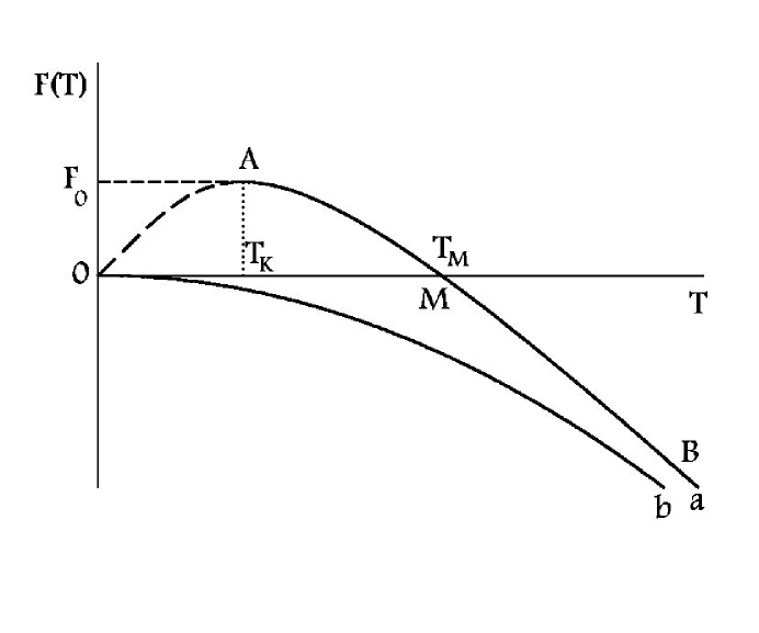
Figure 1: Free energy vs. temperature for a semiflexible polymer: (a) Flory’s calculation; (b) Gujrati-Goldstein upper bound.

Rigorous lower bounds on $\mathit{S}(\mathit{g})$ per particle (and hence upper bounds for the free energy) as a function of $g$ have been obtained [10,11]. Gujrati and Goldstein were able to prove that the entropy per segment of the chain in the case of a single polymer chain that occupies all the sites of the lattice (the Hamilton walk limit) satisfies

$$\mathit{S}(g)\geq\left(\frac{g}{8}\right)\ln(\frac{4}{g}-3).$$ (2)

Hence, S is positive for any value of g $>$0, as it surely must be, in contrast with the results obtained by Flory. Bounds are also available for the case of finite-length polymers [11]. The above bound (2) implies that the equilibrium free energy of the system is never zero for $T>0$, see curve (b) in Fig. 1, and that the system is never completely ordered at any finite temperature.

While the results due to Gujrati and Goldstein clearly show that the approximations of Flory and Huggins do not give a satisfactory description of the system, they just provide an upper bound for the equilibrium free energy of the system; nothing is known about the correct equilibrium entropy. Therefore, it is still unknown what the actual behavior of the free energy is, which is needed to obtain the continuation of the SCL liquid phase. The bounds do not say anything about the extrapolated (i.e. continued) SCL free energy or entropy. The knowledge of the reliable free energy form is fundamental in order to understand if there is a phase transition of any kind in the system at any finite temperature. In particular, it is not clear if the model has a first-order melting transition. It should be recalled that one can usually continue the free energy only past a first-order transition, and not a second order transition due to the singularity in the latter case. If there is no melting transition with a latent heat, then there may be no SCL liquid below the melting transition. In this case, there would be no validity to the Gibbs-DiMarzio conjecture of a  glass transition in the SCL liquid. Thus, an exact calculation is highly desirable.

In recent years, the study of the glass transition has been stimulated by the development of the mode-coupling theory (MCT) [20-22]. This theory was developed in the first place for simple liquids but has been applied to polymers also [20]. The MCT studies the evolution of the density autocorrelation function that can be measured in scattering experiments or calculated in computer simulations and is, therefore, of practical interest. The main result of this theory is the prediction of a critical temperature T_MC, above the glass transition temperature, corresponding to a crossover in the dynamics of the system. At T_MC, the correlation time of the system (the segmental relaxation time in the case of a polymeric glass) diverges with a power law just as one observes near a critical point:

$$\tau\propto\left(T-T_{\mathrm{MC}}\right)^{-\gamma}.$$ (3)

Many neutron and light scattering experiments [20] have shown that the MCT is able to predict at least qualitatively the spectra of low molecular weight materials. Most of the systems for which MCT gives a good description of the dynamics (at least qualitatively) belong to the class of fragile glass formers. The theory has not been tested extensively with polymers that have large molecular weight but at the same time have been shown to be the most fragile systems yet identified [21-23].

Recent activities [24-26] have tried to export the progresses made in the field of spin glasses [33] to the field of real glasses. Even though the replica trick is clearly unphysical [34,35], this approach has been extended to the case of real glasses. The replica approach has been applied to many Lennard-Jones glasses and the results have been interesting [24-26]. They provide some justification for the ideal glass transition. This may also be the case for polymers, which is the focus of this study.

Despite the wide interest in the subject, there is still no comprehensive understanding of the nature of the vitrifying SCL and its relationship with CR, the mechanism responsible for the rapid entropy loss near T_G, and the nature of the ideal glass transition. It would also be interesting to see if there is a possible thermodynamic basis for the critical (and apparently a mode-coupling) transition in SCL’s.

In order to obtain a thermodynamic justification for all these phenomena, we consider in detail in this work a very simple limiting case. The solvent density will be taken to be identically zero. Thus, we consider an incompressible pure system. The effect of free volume is treated in separate publications [29-31]. We also consider the limiting case of a single chain covering the entire lattice. Such a limit is conventionally known as the Hamilton walk limit [10,11]. The case of many chains of finite lengths is considered elsewhere [29-31]. To obtain a first order melting, we have to extend the Flory model of melting, as described below. We have substituted the original square lattice with a Husimi cactus (Fig. 2) on which the original problem is solved exactly. This is the only approximation we make. The results of this calculation for the case of a special interaction have been reported earlier [28] but details were not given. The present work also provides the missing details.

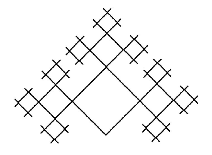
Figure 2: Upper half of a Husimi cactus of generation $m=3$. The dangling bonds outside it show its connection through surface sites (not shown in the figure) with the larger infinite cactus, as explained in the text.

It has been previously shown [36] that the exact calculations on recursive structures like the Husimi cactus are more reliable than conventional mean-field calculations. In this approach, the problem is solved exactly, taking into account all correlations present on the recursive lattice. In most cases, the real lattice is approximated by a tree structure. Because of the tree nature, the correlations are weak. We have chosen the Husimi cactus, obtained by joining two squares (Fig. 2) at each vertex, so that the coordination number $q=4$. On a square lattice, there are also squares that share a bond. Such squares are not present in the cactus. Thus, the cactus should be thought of representing the checkerboard version of the square lattice, with the further provision that no closed loops of size larger than the elementary square are present. The square cactus is chosen to allow for the Gujrati-Goldstein excitations [10,11] that are important in disordering the ideal crystal at absolute zero. The results from the cactus calculation can be thought of as representing an approximate theory of the model on a square lattice.

The layout of the paper is as follows. In the next section, we introduce the lattice model in terms of independent extensive quantities of interest. It is the most general model provided we restrict these quantities to represent pairs, triplets, and quadruplets of sites within each square. We also discuss the general physics of the model. As said above, we use a square lattice for simplicity to introduce the model, even though we eventually consider a Husimi cactus, on which the calculations are exactly. In Sect. III, we explain the recursive solution method on a Husimi cactus. We introduce 1-cycle and 2-cycle solutions, representing the disordered and the ordered phase, respectively. The results are presented in Sect. IV along with the discussion, and the final section contains our conclusions.

2 THE MODEL AND ITS PHYSICS

2.1 Independent extensive quantities

We consider a square lattice of $N$ sites to focus our attention. We will neglect surface effects. There are $N_{\text{B}}=$2$N$ lattice bonds, or distinct pairs of sites. Let us describe the state of a square by the number of polymer bonds $j$ in it. The bonds in the following refer to the polymer bonds. Let $N_{\mathrm{S0}}$, and $N_{\mathrm{S1}}$ denote the number of squares (S) with $j=0$, and 1, respectively; see Fig. 3.

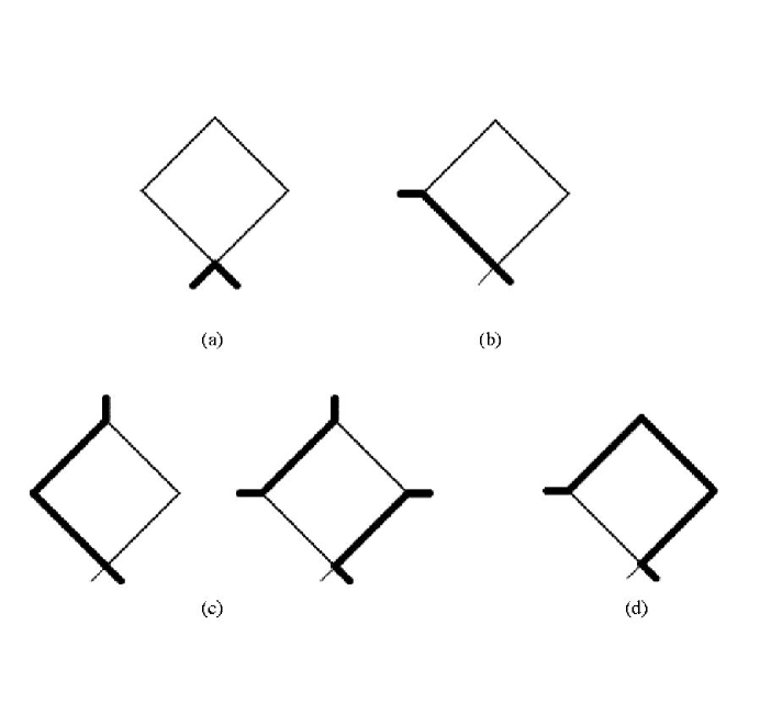
Figure 3: The possible states of a square in the lattice: (a) no bonds, (b) one bond, (c) two bonds and (d) three bonds.

For $j=2$, we distinguish between the case of parallel bonds (p), with the number of such squares $N_{\mathrm{Sp}}$, and gauche (g) bonds, with the number of such squares $N_{\mathrm{Sg}}$. The hairpin (h) turn corresponds to $j=3$, with the number of such squares $N_{\mathrm{Sh}}$. No square is allowed to have four bonds in it. Let $N_{\mathrm{t}}$ and $N_{\mathrm{g}}$ denote the number of trans and gauche bonds, respectively, and $N_{\mathrm{p}}$ and $N_{\mathrm{h}}$ the number of pairs of parallel bonds and hairpin turns, respectively, in a given configuration. We will also use them to represent their average values, as there will be no confusion. It is easily seen that the number of squares on a square lattice is $N_{\mathrm{S}}=N$. Let $B$ denote the number of polymer bonds, and $N_{\mathrm{mm}}$ the number of unbonded monomer-monomer contacts. The following topological identities are easily seen to hold:

$$N_{\text{{S}}}=N_{\mathrm{S0}}+N_{\mathrm{S1}}+N_{\mathrm{Sp}}+N_{\mathrm{Sg}}+N_{\mathrm{Sh}},$$ (4)

$$2N_{\text{{mm}}}=4N_{\mathrm{S0}}+3N_{\mathrm{S1}}+2N_{\mathrm{Sp}}+2N_{\mathrm{Sg}}+N_{\mathrm{Sh}},$$ (5)

$$2B=N_{\mathrm{S1}}+2N_{\mathrm{Sp}}+2N_{\mathrm{Sg}}+3N_{\mathrm{Sh}},$$ (6)

$$N=N_{\mathrm{t}}+N_{\mathrm{g}},\text{ \ }2N=B+N_{\mathrm{mm}},$$ (7)

$$N_{\text{{p}}}=N_{\mathrm{Sp}}+N_{\mathrm{Sh}},\text{ \ }N_{\mathrm{g}}=N_{\mathrm{Sg}}+2N_{\mathrm{Sh}}.$$ (8)

As said earlier, the cactus represents the checkerboard version of the square lattice, so that the number of squares $N_{\text{S}}$ on both lattices with the same number of sites $N$ are not the same; see Sect. III also. For a square lattice, $N_{\text{S}}$= $N$; for the cactus, $N_{\text{S}}$ = $N/2$. However, the number of lattice bonds $N_{\text{B}}$ on both lattices are the same. Because of this, Eq. (6) must be modified for the cactus. Since each bond belongs to only one square in the cactus, we have:

$$B=N_{\mathrm{S1}}+2N_{\mathrm{Sp}}+2N_{\mathrm{Sg}}+3N_{\mathrm{Sh}}.$$ (6a)

All other identities remain valid on the cactus.

2.2 General Model

Among the eleven extensive quantities, $N$, $B$, $N_{\mathrm{g}}$, $N_{\mathrm{t}}$, $N_{\mathrm{mm}}$, $N_{\mathrm{S0}}$, $N_{\mathrm{S1}}$, $N_{\mathrm{Sp}}$, $N_{\mathrm{Sg}}$, $N_{\mathrm{St}}$ and $N_{\mathrm{Sh}}$, there are six independent geometrical relations; the second one in (7) is not independent. In addition, for the Hamilton walk problem, we have $B=N$. Thus, there are only four independent extensive quantities, which we take to be $N$, $N_{\mathrm{g}}$, $N_{\mathrm{p}}$ and $N_{\mathrm{h}}$. One of these, the lattice size $N$, will be used to define the partition function. The remaining three independent quantities $N_{\mathrm{p}}$, $N_{\mathrm{g}}$ and $N_{\mathrm{h}}$ will be then used to define the configuration uniquely. Corresponding to each of the quantities $N_{\mathrm{g}}$, $N_{\mathrm{p}}$ and $N_{\mathrm{h}}$, there is an independent activity $w$, $w_{\mathrm{p}}$ and $w_{\mathrm{h}}$, respectively, that will determine the partition function for the Hamilton walk problem as

$$Z_{N}=\sum w^{N_{\mathrm{g}}}w_{\mathrm{p}}^{N_{\mathrm{p}}}w_{\mathrm{h}}^{N_{\mathrm{h}}},$$ (9a)

where the sum is over distinct configurations obtained by all possible values of $N_{\mathrm{g}}$, $N_{\mathrm{p}}$ and $N_{\mathrm{h}}$ consistent with a fixed lattice size $N$. The activities $w$, $w_{\mathrm{p}}$ and $w_{\mathrm{h}}$ are determined by the three-site bending penalty $\varepsilon$ introduced by Flory in his model, an energy of interaction $\varepsilon_{\mathrm{p}}$ associated with each parallel pair of neighboring bonds, and an energy $\varepsilon_{\mathrm{h}}$ for each hairpin turn within each square as follows:

$$w=\exp\left(-\beta\varepsilon\right),\ w_{\mathrm{p}}=\exp\left(-\beta\varepsilon_{\mathrm{p}}\right),\ w_{\mathrm{h}}=\exp(-\beta\varepsilon_{\mathrm{h}}).$$

Here, $\beta$ is the inverse temperature T in the units of the Boltzmann constant. The original Flory model is obtained when the last two interactions are absent. It should be stressed that $\varepsilon_{\mathrm{h}}$ is the excess energy associated to the configuration, once the energy of the two bends and the pair of parallel bonds have been subtracted out. Both $\varepsilon_{\mathrm{p}}$ and $\varepsilon_{\mathrm{h}}$ are associated with four-site interactions, since it is necessary to determine the state of four adjacent sites to determine if a pair of parallel bonds or a hairpin turn is present.

The model is easily generalized to include free volume by introducing voids, each of which occupies a site of the lattice. The number of voids $N_{0}$ is controlled by the void activity $\eta$. The number $P$ of polymers is controlled by another activity given by $H^{2}.$ The interaction between nearest neighbor pairs $N_{\text{c}}$ of voids and the monomers of the polymers determines the Boltzmann weight $w_{\text{c}}$. The partition function of the extended model is given by

$$Z_{N}=\sum\eta^{N_{0}}H^{2P}w_{\text{c}}^{N_{\text{c}}}w^{N_{\mathrm{g}}}w_{\mathrm{p}}^{N_{\mathrm{p}}}w_{\mathrm{h}}^{N_{\mathrm{h}}},$$ (9b)

where the sum is over distinct configurations consistent with the fixed lattice of $N$ sites. Because the activity $H$ only determines the average number of linear polymers, but not their individual sizes, the model in Eq. (9b) describes polydisperse polymers [37], each of which must contain at least one bond.

We now turn to our simplified model of the Hamilton walk ($P=1$, and $\ N_{0}=0$). In this model, the energy of interaction in a given configuration is given by

$$\mathcal{E}=\varepsilon N_{\mathrm{g}}+\varepsilon_{\mathrm{p}}N_{\mathrm{p}}+\varepsilon_{\mathrm{h}}N_{\mathrm{h}}=\varepsilon\left(N_{\mathrm{g}}+aN_{\mathrm{p}}+bN_{\mathrm{h}}\right),$$ (10)

where $a\equiv\varepsilon_{\mathrm{p}}/\varepsilon$, $b\equiv\varepsilon_{\mathrm{h}}/\varepsilon$. The parameters can in principle assume positive and negative values. However, we will restrict ourselves to $\varepsilon>0$ in this work. The limit $\varepsilon=\varepsilon_{\text{p}}=\varepsilon_{\text{h}}=0$ corresponds to a completely flexible polymer problem, which is of no interest to us here, as it corresponds to the infinite temperature limit of our model. The limit, however, is of considerable interest in the study of protein folding and has been investigated by several workers [38]. In addition, we will focus mainly on the case $0<a<1$. A positive $a$ guarantees that parallel bond energy opposes the creation of configurations in which pairs of parallel bonds are present and $a<1$ makes the penalty for a pair of parallel bonds less than that for a gauche conformation. This guarantees the presence of a crystalline phase at low temperatures, as shown below.

2.3 Ground State at $\mathit{T}$=0

The physics of the model at absolute zero can be easily understood on general grounds. We are interested in the thermodynamic limit $N\rightarrow\infty$. We first consider $b=0$. For $a<1$, the ground state at $T=0$ has $N_{\mathrm{g}}=0$, $N_{\mathrm{p}}=N$, $N_{\mathrm{h}}=0$, as shown in Fig. 4(a). (The labels R and L are related to the state of the sites as introduced in the next section.) Thus, $\mathcal{E}=\varepsilon_{\text{p}}N$. This is what we will call the perfect crystal at absolute zero. For $b\neq 0$, the state in Fig. 4(a) remains the ground state as long as $2+b>0$. This condition ensures that hairpin turns are not present. For $a>1$, and $b=0$, the ground state at $T=0$ has $N_{\mathrm{g}}=N$, $N_{\mathrm{p}}=0$, as shown in Fig. 4(b). Thus, $\mathcal{E}=\varepsilon N$. This remains the ground state provided $a+b>0$, which ensures that the hairpin turns are not present. Since our interest is to have a crystal state as the equilibrium state at low temperatures, we would only consider the earlier case $a<1$, with $2+b>0$.

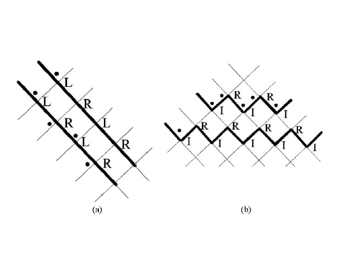
Figure 4: Possible configurations of the polymer chain at $T=0$: (a) crystalline phase with $N_{\mathrm{g}}=0$ and $N_{\mathrm{p}}=N$; (b) step-like configuration with $N_{\mathrm{p}}=0$ and $N_{\mathrm{g}}=N$. See text for the explanation of the symbols.

It should be recognized that the model considered here is defined on a lattice. Thus, the ground state also possesses the symmetry of the lattice. This symmetry is imposed by the lattice symmetry and is independent of the model. Thus, this induced symmetry should not be confused with the point group symmetry of a real crystal, which is brought about by the interactions in the system. The symmetry in our model is due to the orientational order between pairs of parallel bonds. It is because of the orientational order defining the crystal in our model that we can obtain a continuous transition between the crystal and the equilibrium liquid.

The lack of a point group symmetry of a real crystal in our model should not be a taken as a serious limitation of the model, since our main goal is to study the possibility of a glass transition in a supercooled liquid. The determination of the supercooled liquid branch requires the continuation past a first-order melting transition. Thus, the exact nature of the symmetry of the CR phase is not as important as the existence of a discontinuous melting.

3 RECURSIVE SOLUTION

The Husimi cactus approximates the square lattice, as said above. Both have the coordination number $q=4$, and the elemental squares as the smallest loop. However, the most important reason for choosing the square cactus is that it allows for hairpin turns that give rise to the Gujrati-Goldstein excitation in the Flory model of melting. A Bethe lattice would be inappropriate for this reason. As said above, the number of squares on the cactus is half of that on a square lattice with the same number of sites $N$. This can also be easily seen as follows by assuming homogeneity of the lattice. First, consider the square lattice. Four squares meet at each site; however, each square will be counted four times, due to its four corners, assuming homogeneity. Thus, $N_{\mathrm{S}}=N$. On a cactus, only two squares meet, but each one is counted four times as before. Hence, $N_{\mathrm{S}}=N/2$. Despite this, $N_{\mathrm{B}}=2N$ on both lattices, only half of which are going to be taken up by the Hamilton walk on both lattices.

A site is shared by four bonds and two squares $\Sigma$, and $\Sigma^{\prime}$ that are across from each other on the cactus. On the other hand, there are two different pairs of such squares on a square lattice. In a formal sense, we can imagine that each end of a bond contributes $\frac{1}{4}$ of a site, and each corner of a square contributes $\frac{1}{2}$ of a site (on a square lattice each corner contributes $\frac{1}{4}$ of a site.). This formal picture will be useful in determining the nature of a homogeneous cactus. To make the cactus homogeneous, we must consider it to be part of a larger cactus. This is shown in Fig. 2, where we show a cactus of generation $m=3$ with dangling bonds (each one ending with a surface site, not shown in the figure) outside it to show its connection with the larger infinite cactus. The latter has no boundary. A similar homogeneity hypothesis associated with a Bethe lattice has been discussed in Ref. 37(b) to which we refer the reader for further details. On a Bethe lattice, each dangling bond was treated as a half-bond to ensure that $N_{\mathrm{B}}=qN/2$, where $q$ is the coordination number of the Bethe lattice. For the case of the cactus, we treat each pair of dangling bonds in Fig. 2 as a half-square, and each surface site as a half-site to calculate the number of sites $N_{m}$, and the number of squares $S_{m}$ for a cactus of $m$ generations. A trivial calculation shows that

$$N_{m}=4\times 3^{m}-2,\text{ \ \ }S_{m}=2\times 3^{m}-1,$$ (11)

so that $S_{m}=N_{m}/2$, as $m\rightarrow\infty$. Since each square contributes 4 bonds, it is also evident that $N_{\mathrm{B}}=2N$ in the limit of an infinite cactus. A detailed calculation of the quantities introduced above is given in the Appendix.

Because of the above-mentioned homogeneity, a site is arbitrarily designated as the origin of the cactus. Each square has one site, called the base site, closer to the origin. The base site is given an index $m\geq 0$ , the two sites next to the base site within the square, called the intermediate sites, the index $(m+1)$, and the remaining fourth site, called the peak site, the index $(m+2)$. We will call this square an $m$th level square; it has its base at the $m$th level and its peak at the $(m+2)$th level; see Fig. 5. The two lower bonds in the $m$th square connected to the $m$th site are called the lower bonds and the two upper bonds connected to the peak site are called the upper bonds. The origin of the lattice is labeled as the $m=0$ level and the level index $m$ increases as we move outwards from the origin. We can imagine cutting the Husimi tree at an $m$th site into two parts, one of which does not contain the origin if $m>0$. We call this the $m$th branch of the lattice and denote it by $\mathcal{C}_{m}$. At the origin, we get two identical branches each containing the origin. We will call each of those the $(m=0)$th branch.

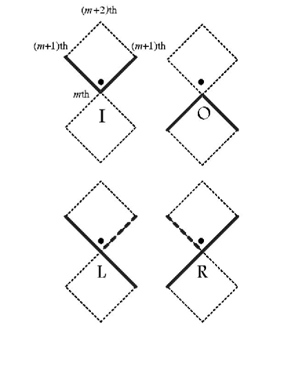
Figure 5: The four possible states of the polymer chain at any site at the $m$th level of the lattice.

We only consider parallel bonds and hairpin turns that are inside the squares, since the cactus represents the checkerboard version of the square lattice. Thus, each square can contribute only once to either $N_{\text{p}}$, or $N_{\text{h}}.\;$This means that $N_{\text{p}}=N_{\text{S}}=N/2$ in the perfect crystal at absolute zero. Similarly, it can be easily seen that the maximum possible value of $N_{\text{h}}\;$is $2N_{\text{S}}/3=N/3$.

3.1 Recursion Relations

We consider a linear polymer that covers all the sites of the Husimi cactus or the square. Its configuration determines the state of the bonds in each square. Consider a pair of two squares $\Sigma$, and $\Sigma^{\prime}\,$that are across from each other. We distinguish $\Sigma$ by putting a filled dot ($\bullet$) just above the common site. We now face towards $\Sigma^{\prime}$ from within $\Sigma$ through this common site. The common site has been taken as the base site in Fig. 5, but the following description is valid at any site. The common site can assume 4 possible different states depending on the state of the four bonds connected to it. Two of the bonds are in $\Sigma,$ and the remaining two are in $\Sigma^{\prime}.$

1. In the I state, both $\Sigma$- bonds are occupied by the polymer chain. Since the polymer is linear, the two $\Sigma^{\prime}$-bonds must be unoccupied by the polymer.

2. In the O state, both $\Sigma$-bonds are unoccupied but both $\Sigma^{\prime}$-bonds are occupied by the polymer chain.

3. In the L state, only one of the $\Sigma$-bonds is occupied and the polymer occupies the left bond in $\Sigma^{\prime}$ (we always think about left and right as we face towards $\Sigma$’).

4. In the R state, only one of the $\Sigma$-bonds is occupied and the polymer occupies the right bond in $\Sigma^{\prime}$.

For the common site at $m=0$, the square $\Sigma^{\prime}$ in the above classification is the square on the other side of the origin.

It is now easy to understand the labeling of the two configurations shown in Fig. 4.

We are interested in the contribution of the portion of the $m$th branch $\mathcal{C}_{m}$ of the lattice to the total partition function of the system. This contribution is called the partial partition function (PPF) of the branch. It is easy to see that the PPF depends on the state $\alpha$ of the $m$th level site. We denote this PPF by $Z_{m}(\alpha)$. We now wish to express $Z_{m}(\alpha)$ recursively in terms of the PPF’s of the two intermediate sites and the peak site of the $m$th square. Following Gujrati [36], the recursion relations can always be written in the form:

$$Z_{m}(\alpha)=\text{Tr}[\text{W}(\alpha,\left\{\beta\right\})Z_{m+1}(\beta_{1})Z_{m+1}(\beta_{2})Z_{m+2}(\beta_{3})],$$ (12)

where $\left\{\beta\right\}$ is the set of states $\beta_{i}$; the latter states represent the possible states of the other three sites of the square, and W$(\alpha,\left\{\beta\right\})$ is the local Boltzmann weight of the square due to conformation of the polymer chain inside the square.

Let us consider in detail the case in which the base site at the $m$th level is in the I state. The three possible configurations that the polymer can assume in the $m$th level square are shown in Fig. 6.

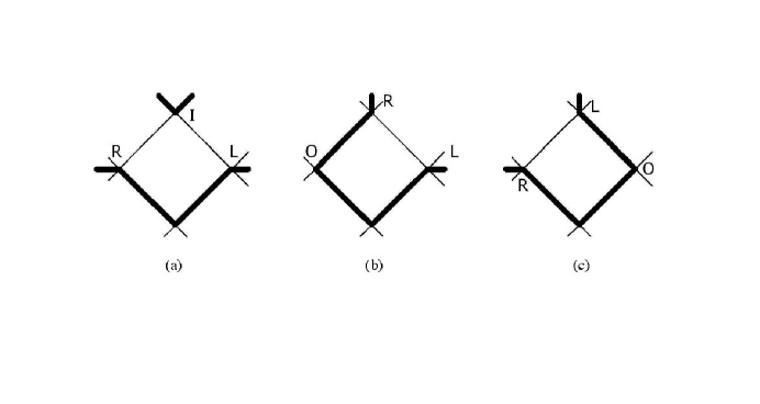
Figure 6: Possible configurations of the polymer chain when the $m$th level site is in the I state.

In this figure, L, R, I and O represent the possible state of the $(m+1)$th and $(m+2)$th level sites and $w$ represents the weight of a bend. In order to carefully account for statistical weights, a Boltzmann weight equal to $w$ is considered only if the bend happens:

1. At the $m$th level and at least one polymer bond at the level is inside the square.

2. At the $(m+1)$th or $(m+2)$th level, and both polymer bonds at the level are inside the polymer.

A weight $w_{\mathrm{p}}=w^{a}$ is considered for any configuration in which two bonds are parallel to each other within the same square. We can, furthermore, distinguish configurations in which two bonds are parallel to each other from configurations, like those shown in Figs. 6(b)-(c), where three consecutive bonds form a hairpin configuration. Whenever this configuration is present, an additional weight $w_{\mathrm{h}}=w^{b}$ is introduced.

It is not important to know along which of the two lower bonds in the $(m+1)$th or $(m+2)$th square does the polymer chain enter into the $m$th square. In fact, even if the polymer undergoes a bend while moving from the higher level square to the $m$th level square, the corresponding weight is already taken into account into the partial partition function of the higher level site.

It is important to consider always the state of a site moving through the lattice towards the origin. In the configuration in Fig. 6(a), the intermediate site on the left is in the R state since the polymer undergoes a right turn after entering the square. The intermediate site on the right is in the L state since the polymer undergoes a left turn after entering the square. Finally, the peak site is in the I state because the polymer is coming from the $(m+1)$th level square but not entering the $m$th level square. The polymer undergoes one bend (at the base site) so that there is a weight $w$ to be taken into account. Thus the contribution to the partition function coming from this configuration is:

$$wZ_{m+1}(\mathrm{R})Z_{m+1}(\mathrm{L})Z_{m+2}(\mathrm{I}).$$ (13)

In the configuration in Fig. 6(b), the intermediate site on the left is in the O state since both the lower bonds in the corresponding $(m+1)$th square are unoccupied. The intermediate site on the right is in the L state since the polymer undergoes a left turn after entering the square. Finally, the peak site is in the R state since the polymer undergoes a right turn after entering the square. The polymer undergoes two bends (one at the base site and the other one at the left intermediate site) so that there is a weight $w^{2}$ to be taken into account. There is a pair of parallel bonds in the square and a hairpin turn occurs so that a weight $w_{\mathrm{h}}w_{\mathrm{p}}$ has also to be taken into account. Thus, the contribution to the partition function coming from this configuration is:

$$w^{2}w_{\mathrm{h}}w_{\mathrm{p}}Z_{m+1}(\mathrm{O})Z_{m+1}(\mathrm{L})Z_{m+2}(\mathrm{R}).$$ (14)

In the configuration in Fig. 6(c), the intermediate site on the right is in the O state since both the lower bonds in this particular $(m+1)$th square are unoccupied. The intermediate site on the left is in the R state since the polymer undergoes a right turn after entering the square. Finally, the peak site is in the L state since the polymer undergoes a left turn after entering the square. The polymer undergoes two bends (one at the base site and the other one at the right intermediate site) so that there is a weight $w^{2}$ to be taken into account. We also have a pair of parallel bonds and a hairpin turn to take into account in this case. Thus, the contribution to the partition function coming from this configuration is:

$$w^{2}w_{\mathrm{h}}w_{\mathrm{p}}Z_{m+1}(\mathrm{O})Z_{m+1}(\mathrm{R})Z_{m+2}(\mathrm{L}).$$ (15)

The recursion relation for $Z_{m}(\mathrm{I})$, the partition function of the $m$th branch of the Husimi tree given that the $m$th level site is in the I state, is therefore given by:

$$Z_{m}(\mathrm{I}) =w^{2}w_{\mathrm{h}}w_{\mathrm{p}}Z_{m+1}(\mathrm{O})[Z_{m+1}(\mathrm{L})Z_{m+2}(\mathrm{R})+Z_{m+1}(\mathrm{R})Z_{m+2}(\mathrm{L})]$$

$$+wZ_{m+1}(\mathrm{R})Z_{m+1}(\mathrm{L})Z_{m+2}(\mathrm{I}).$$ (16)

Considering the case in which the $m$th level site is in the O state, the partial partition function $Z_{m}(\mathrm{O})$ for the O state can be written as:

$$Z_{m}(\mathrm{O}) =Z_{m+1}^{2}(\mathrm{I})Z_{m+2}(\mathrm{I})+Z_{m+1}(\mathrm{I})\left[Z_{m+1}(\mathrm{L})Z_{m+2}(\mathrm{R})+Z_{m+1}(\mathrm{R})Z_{m+2}(\mathrm{L})\right]$$

$$+wZ_{m+1}(\mathrm{R})Z_{m+1}(\mathrm{L})Z_{m+2}(\mathrm{O}).$$ (17)

When the $m$th level site is in the L state the partial partition function can be written as:

$$Z_{m}(\mathrm{L}) =[Z_{m+1}(\mathrm{R})+wZ_{m+1}(\mathrm{L})]\{Z_{m+1}(\mathrm{I})Z_{m+2}(\mathrm{I})+w^{2}w_{\mathrm{p}}w_{\mathrm{h}}Z_{m+1}(\mathrm{O})Z_{m+2}(\mathrm{O})\}$$

$$+w_{\mathrm{p}}\left[wZ_{m+1}^{2}(\mathrm{L})Z_{m+2}(\mathrm{R})+Z_{m+1}^{2}(\mathrm{R})Z_{m+2}(\mathrm{L})\right]$$

$$+\left[Z_{m+2}(\mathrm{R})+wZ_{m+2}(\mathrm{L})\right]wZ_{m+1}(\mathrm{I})Z_{m+1}(\mathrm{O}).$$ (18)

The relation for the R state is obtained from $Z_{m}(\mathrm{L})$ by the interchange L$\longleftrightarrow$R:

$$Z_{m}(\mathrm{R}) =[Z_{m+1}(\mathrm{L})+wZ_{m+1}(\mathrm{R})]\{Z_{m+1}(\mathrm{I})Z_{m+2}(\mathrm{I})+w^{2}w_{\mathrm{p}}w_{\mathrm{h}}Z_{m+1}(\mathrm{O})Z_{m+2}(\mathrm{O})\}$$

$$+w_{\mathrm{p}}\left[wZ_{m+1}^{2}(\mathrm{R})Z_{m+2}(\mathrm{L})+Z_{m+1}^{2}(\mathrm{L})Z_{m+2}(\mathrm{R})\right]$$

$$+\left[Z_{m+2}(\mathrm{L})+wZ_{m+2}(\mathrm{R})\right]wZ_{m+1}(\mathrm{I})Z_{m+1}(\mathrm{O}).$$ (19)

It is possible to write analogous relations for $Z_{m+1}(\mathrm{\alpha})$ by properly substituting $m\rightarrow m+1,$ $m+1\rightarrow m+2$ and $m+2\rightarrow m+3.$ We introduce the following ratios between partial partition functions at even and odd levels of the lattice:

$$x_{m}(\mathrm{I}) =Z_{m}(\mathrm{I})/\left(Z_{m}(\mathrm{L})+Z_{m}(\mathrm{R})\right),$$

$$x_{m}(\mathrm{O}) =Z_{m}(\mathrm{O})/\left(Z_{m}(\mathrm{L})+Z_{m}(\mathrm{R})\right),$$

$$x_{m}(\mathrm{L}) =Z_{m}(\mathrm{L})/\left(Z_{m}(\mathrm{L})+Z_{m}(\mathrm{R})\right),$$

$$x_{m}(\mathrm{R}) =1-x_{m}(\mathrm{L}).$$ (20)

As one moves from a level that is infinitely far away from the origin towards the origin itself, the recursion relations (16)-(19) will approach fix-point (FP) solutions, $x_{m}(\alpha)\rightarrow x^{\ast}(\alpha)$, $x_{m+1}(\alpha)\rightarrow x^{\ast\ast}(\alpha)$, etc., where $\alpha=$ I, O, L or R. These fix-point solutions of the recursion relations describe the behavior in the interior of the Husimi tree. Once the fixed point is reached, the value of $x^{\ast}(\alpha)$ and $x^{\ast\ast}(\alpha)$ becomes independent of $m.$ On a Husimi cactus, a site can be classified as a simultaneous peak and a base site, or a simultaneous peak and a middle site, depending on the pair of squares which share the site. Thus, it is expected that the most general FP solutions will correspond to a 2-cycle solution in which $\ x_{m}(\alpha)$ and $x_{m+2}(\alpha)\;$tend to the same limit. In this case, we obtain a sublattice structure in which sites with even levels are different from sites with odd levels. We can write in this case:

$$x_{m}(\mathrm{I}) =x_{m+2}(\mathrm{I})=i_{\mathrm{a}},\;x_{m}(\mathrm{O})=x_{m+2}(\mathrm{O})=o_{\mathrm{a}},\;x_{m}(\mathrm{L})=x_{m+2}(\mathrm{L})=l_{\mathrm{a}},$$

$$x_{m}(\mathrm{R}) =x_{m+2}(\mathrm{R})=1-x_{m}(\mathrm{L})=1-l_{\mathrm{a}},$$

$$x_{m+1}(\mathrm{I}) =x_{m+3}(\mathrm{I})=i_{\mathrm{b}},\;x_{m+1}(\mathrm{O})=x_{m+3}(\mathrm{O})=o_{\mathrm{b}},\;x_{m+1}(\mathrm{L})=x_{m+3}(\mathrm{L})=l_{\mathrm{b}},$$

$$x_{m+1}(\mathrm{R}) =x_{m+3}(\mathrm{R})=1-x_{m+1}(\mathrm{L})=1-l_{\mathrm{b}}.$$ (21)

The indices a and b refer to even and odd levels, respectively. Using (21), it is easy to prove that the system of equations (16) to (19) can be written in the following form:

$$i_{\mathrm{a}}Q_{\mathrm{LR}} =w\left(1-l_{\mathrm{b}}\right)l_{\mathrm{b}}i_{\mathrm{a}}+w^{2}w_{\mathrm{p}}w_{\mathrm{h}}o_{\mathrm{b}}\left[l_{\mathrm{b}}(1-l_{\mathrm{a}})+l_{\mathrm{a}}(1-l_{\mathrm{b}})\right],$$ (22)

$$o_{\mathrm{a}}Q_{\mathrm{LR}} =i_{\mathrm{b}}^{2}i_{\mathrm{a}}+i_{\mathrm{b}}\left[l_{\mathrm{b}}(1-l_{\mathrm{a}})+l_{\mathrm{a}}(1-l_{\mathrm{b}})\right]+w(1-l_{\mathrm{b}})l_{\mathrm{b}}o_{\mathrm{a}},$$ (23)

$$l_{\mathrm{a}}Q_{\mathrm{LR}} =(1-l_{\mathrm{b}}+wl_{\mathrm{b}})[i_{\mathrm{b}}i_{\mathrm{a}}+w^{2}w_{\mathrm{p}}w_{\mathrm{h}}o_{\mathrm{b}}o_{\mathrm{a}}]$$

$$+wo_{\mathrm{b}}i_{\mathrm{b}}(1-l_{\mathrm{a}}+wl_{\mathrm{a}})+w_{\mathrm{p}}(1-l_{\mathrm{b}})^{2}l_{\mathrm{a}}+ww_{\mathrm{p}}l_{\mathrm{b}}^{2}(1-l_{\mathrm{a}}),$$ (24)

$$i_{\mathrm{b}}Q_{\mathrm{LR}}^{{}^{\prime}} =w\left(1-l_{\mathrm{a}}\right)l_{\mathrm{a}}i_{\mathrm{b}}+w^{2}w_{\mathrm{p}}w_{\mathrm{h}}o_{\mathrm{a}}\left[l_{\mathrm{a}}(1-l_{\mathrm{b}})+l_{\mathrm{b}}(1-l_{\mathrm{a}})\right],$$ (25)

$$o_{\mathrm{b}}Q_{\mathrm{LR}}^{{}^{\prime}} =i_{\mathrm{a}}^{2}i_{\mathrm{b}}+i_{\mathrm{a}}\left[l_{\mathrm{a}}(1-l_{\mathrm{b}})+l_{\mathrm{b}}(1-l_{\mathrm{a}})\right]+w(1-l_{\mathrm{a}})l_{\mathrm{a}}o_{\mathrm{b}},$$ (26)

$$l_{\mathrm{b}}Q_{\mathrm{LR}} =(1-l_{\mathrm{a}}+wl_{\mathrm{a}})[i_{\mathrm{a}}i_{\mathrm{b}}+w^{2}w_{\mathrm{p}}w_{\mathrm{h}}o_{\mathrm{a}}o_{\mathrm{b}}]$$

$$+wo_{\mathrm{a}}i_{\mathrm{a}}(1-l_{\mathrm{b}}+wl_{\mathrm{b}})+w_{\mathrm{p}}(1-l_{\mathrm{a}})^{2}l_{\mathrm{b}}+ww_{\mathrm{p}}l_{\mathrm{a}}^{2}(1-l_{\mathrm{b}}),$$ (27)

where $Q_{\mathrm{LR}}^{{}^{\prime}}$ is obtained from $Q_{\mathrm{LR}}$ by exchanging a and b subscripts and $Q_{\mathrm{LR}}$ can be written as:

$$Q_{\mathrm{LR}}=\left(1+w\right)\{i_{\mathrm{b}}i_{\mathrm{a}}+w^{2}w_{\mathrm{p}}w_{\mathrm{h}}o_{\mathrm{b}}o_{\mathrm{a}}+wi_{\mathrm{b}}o_{\mathrm{b}}+w_{\mathrm{p}}[l_{\mathrm{b}}(1-l_{\mathrm{a}})^{2}+l_{\mathrm{a}}(1-l_{\mathrm{b}})^{2}]\}.$$ (28)

3.2 2-cycle Free Energy

In order to determine which phase is the stable one at some temperature, we have to find the free energy of all the possible phases of the system as a function of $w$. We follow the treatment by Gujrati [36], and provide its trivial extension to the 2-cycle FP solution shown above. The free energy per site at the origin of the lattice can be easily calculated from the expressions for the total partition function $Z$ at the $(m=0)$th, $(m=1)$th and $(m=2)$th levels.

The total partition function of the system $Z_{0}$ can be written by considering the two $(m=0)$th branches $\mathcal{C}_{0}\;$meeting at the origin at the $(m=0)$th level. For this, we need to consider all the possible configurations in the two branches. This is done by considering all the configurations that the polymer chain can assume in the two squares that meet at the origin of the tree. All the possible configurations of the $(m=0)$th level site (in this case we are not interested in the state of the $(m=1)$th level sites) are shown in Fig. 7.

Figure 7: Possible configurations of the polymer chain at the origin of the tree.

Each of the first two configurations contributes

$$Z_{0}(\mathrm{I})Z_{0}(\mathrm{O})$$

to the total partition function. The third and fourth configurations both contribute

$$(1/w)Z_{0,\mathrm{g}}(\mathrm{L})Z_{0,\mathrm{g}}(\mathrm{R}),$$

where the factor $(1/w)$ is needed in order not to take into account the Boltzmann weight at the origin twice and the subscripts ”g” and ”t” refer to the gauche and trans part of the partition function for L and R states. In fact, it is possible to separate these two contributions to the partition function at any level. The ”gauche” portion is the one corresponding to configurations such that there is a bending at the $m$th level site, while the ”trans” portion is the one corresponding to configurations in which the two bonds coming out of the $m$th level site that we are considering are straight. It is easily seen that:

$$Z_{m,\mathrm{t}}(\mathrm{L}) =Z_{m+1}(\mathrm{R})\{Z_{m+1}(\mathrm{I})Z_{m+2}(\mathrm{I})+w^{2}w_{\mathrm{p}}w_{\mathrm{h}}Z_{m+1}(\mathrm{O})Z_{m+2}(\mathrm{O})$$

$$+w_{\mathrm{p}}Z_{m+1}(\mathrm{R})Z_{m+2}(\mathrm{L})\}+wZ_{m+2}(\mathrm{R})Z_{m+1}(\mathrm{I})Z_{m+1}(\mathrm{O}),$$ (29)

and

$$Z_{m,\mathrm{g}}(\mathrm{L}) =wZ_{m+1}(\mathrm{L})\{Z_{m+1}(\mathrm{I})Z_{m+2}(\mathrm{I})+w^{2}w_{\mathrm{p}}w_{\mathrm{h}}Z_{m+1}(\mathrm{O})Z_{m+2}(\mathrm{O})$$

$$+w_{\mathrm{p}}Z_{m+1}(\mathrm{L})Z_{m+2}(\mathrm{R})\}+w^{2}Z_{m+2}(\mathrm{L})Z_{m+1}(\mathrm{I})Z_{m+1}(\mathrm{O}).$$ (30)

Finally, the fifth and sixth configurations contribute $Z_{0,\mathrm{t}}^{2}(\mathrm{L})$ and $Z_{0,\mathrm{t}}^{2}(\mathrm{R})$, respectively. It is then possible to write:

$$Z_{0}=2Z_{0}(\mathrm{I})Z_{0}(\mathrm{O})+(2/w)Z_{0,\mathrm{g}}(\mathrm{L})Z_{0,\mathrm{g}}(\mathrm{R})+Z_{0,\mathrm{t}}^{2}(\mathrm{L})+Z_{0,\mathrm{t}}^{2}(\mathrm{R}).$$ (31)

It is clear that $Z_{0}$ is the total partition function of the system obtained by joining two branches $\mathcal{C}_{0}$ together at the origin. Now, let us imagine taking away from the lattice the two squares that meet at the origin. This leaves behind four different branches $\mathcal{C}_{1}$ and two branches $\mathcal{C}_{2}$. We connect the two $\mathcal{C}_{2}$ branches to form a smaller cactus whose partition function is denoted by $Z_{2}$. Similarly, we join two of the $\mathcal{C}_{1}$ branches to form an intermediate cactus whose partition function is denoted by $Z_{1}$. We can form two such intermediate cacti out of the four $\mathcal{C}_{1}$ branches. Each partition function $Z_{1}$ or $Z_{2}$ can be written in a form that is identical to that of Equation (31):

$$Z_{i}=2Z_{i}(\mathrm{I})Z_{i}(\mathrm{O})+(2/w)Z_{i,\mathrm{g}}(\mathrm{L})Z_{i,\mathrm{g}}(\mathrm{R})+Z_{i,\mathrm{t}}^{2}(\mathrm{L})+Z_{i,\mathrm{t}}^{2}(\mathrm{R}),$$ (32)

where $i=1,2.$

The difference between the free energy of the complete cactus and that of the three reduced cacti is just the free energy corresponding to a pair of squares so that, following Gujrati [36], we can write the adimensional free energy per square (without the conventional minus sign) as:

$$\omega\equiv\omega_{\text{sq}}=\frac{1}{2}\ln[Z_{0}/\{Z_{1}^{2}Z_{2}\}].$$ (33)

It is possible to write:

$$Z_{0}=B_{0}^{2}Q_{2}(i_{\mathrm{a}},o_{\mathrm{a}},l_{\mathrm{a}},i_{\mathrm{b}},o_{\mathrm{b}},l_{\mathrm{b}}),$$ (34)

$$Z_{1}=B_{1}^{2}Q_{2}^{{}^{\prime}}(i_{\mathrm{a}},o_{\mathrm{a}},l_{\mathrm{a}},i_{\mathrm{b}},o_{\mathrm{b}},l_{\mathrm{b}}),$$ (35)

$$Z_{2}=B_{2}^{2}Q_{2}(i_{\mathrm{a}},o_{\mathrm{a}},l_{\mathrm{a}},i_{\mathrm{b}},o_{\mathrm{b}},l_{\mathrm{b}}),$$ (36)

where we have introduced

$$B_{m}=Z_{m}(\mathrm{L})+Z_{m}(\mathrm{R}),$$ (37)

and where $Q_{2}$ is the following polynomial of $i_{\mathrm{a}},o_{\mathrm{a}},l_{\mathrm{a}},i_{\mathrm{b}},o_{\mathrm{b}}$ and $l_{\mathrm{b}}$:

$$Q_{2}=2i_{\mathrm{a}}o_{\mathrm{a}}+(2/w)l_{\mathrm{a,g}}(1-l_{\mathrm{a}})_{\text{{g}}}+l_{\mathrm{a,t}}^{2}+(1-l_{\mathrm{a}})_{\mathrm{t}}^{2};$$ (38)

$l_{\mathrm{a,t}}$ and $l_{\mathrm{a,g}}$ correspond to the trans and gauche portions of $l_{\mathrm{a}}$, respectively, and $Q_{2}^{{}^{\prime}}$

is obtained from $Q_{2}$ by interchanging a and b subscripts.

It is also easily seen that:

$$B_{0}=B_{1}^{2}B_{2}Q_{\mathrm{LR}}(i_{\mathrm{a}},o_{\mathrm{a}},l_{\mathrm{a}},i_{\mathrm{b}},o_{\mathrm{b}},l_{\mathrm{b}}).$$ (39)

so that the free energy per square can be written as:

$$\omega\equiv\omega_{\text{sq}}=\ln\left(\frac{Q_{\mathrm{LR}}}{Q_{2}^{{}^{\prime}}}\right).$$ (40a)

The free energy per site $\omega_{\text{site}}$ is proportional to $\omega_{\text{sq}}:$

$$\omega_{\text{site}}\equiv\omega_{\text{sq}}/2,$$ (40b)

since there are two sites per square.

The usual Helmholtz free energy per square can be obtained from $\omega$ through:

$$F=-T\omega.$$ (41)

If it happens that the even and odd sites are not different, we obtain a 1-cycle FP-solution. Below, we will consider the two solutions separately.

3.3 1-cycle solution

In the 1-cycle scheme, we have $x_{m}(\alpha)=x_{m+1}(\alpha)$ as they converge to the same fix point. Thus, we have: $i_{\mathrm{a}}=i_{\mathrm{b}}=i$, $o_{\mathrm{a}}=o_{\mathrm{b}}=o$ and $l_{\mathrm{a}}=l_{\mathrm{b}}=l.\;$In this case the system of equations reduces to:

$$iQ_{\mathrm{LR}} =w\left(1-l\right)li+2w^{2}w_{\mathrm{p}}w_{\mathrm{h}}ol(1-l),$$ (42)

$$oQ_{\mathrm{LR}} =i^{3}+2il(1-l)+w(1-l)lo,$$ (43)

$$lQ_{\mathrm{LR}} =\left[(1-l)+wl\right]\left\{i^{2}+w^{2}w_{\mathrm{p}}w_{\mathrm{h}}o^{2}+w_{\mathrm{p}}l(1-l)+wio\right\},$$ (44)

with:

$$Q_{\mathrm{LR}}=(1+w)\left\{i^{2}+w^{2}w_{\mathrm{p}}w_{\mathrm{h}}o^{2}+w_{\mathrm{p}}l(1-l)+wio\right\}.$$ (45)

From (44), it is easy to show that we must have $l=\frac{1}{2}$ for every solution obtained in this scheme.

One solution that exists for every value of $w$ (and, hence, of $T$) is the following:

$$l=\frac{1}{2},o=0,i=0.$$ (46)

This represents a liquid-like phase without any I, or O states. We label this phase metastable liquid (ML) because, as we will show below, it never represents the equilibrium phase of the system even though it exists at all temperatures. For large enough $w$, there is another solution of the system of equations with nonzero values for $o$ and $i$, and it has to be found numerically. We label this second liquid-like phase equilibrium liquid (EL) since, as our free energy calculations will show, it represents the equilibrium phase of the system at high temperature. The temperature at which EL appears is a function of $w_{\mathrm{p}}$ and $w_{\mathrm{h}}$. We will call the temperature $T_{\mathrm{MC}}$, at which the equilibrium liquid appears, the mode coupling temperature for reasons that will become clear below.

Table 1 shows how the value of $T_{\mathrm{MC}}$ changes as a function of $a$ (both positive and negative values of $a$ are considered, see below) as we keep $b$ equal to zero.

a	$T_{\text{MC}}$
-1	2.9586
-0.8	2.6183
-0.5	2.1876
-0.2	1.7359
0	1.4427
0.2	1.1600
0.5	0.7653
0.8	0.4156
1	0

Table 1: Values of $T_{\mathrm{MC}}$ as a function of $a$ (with $b=0$).

For the ML, we have $o=i=0,l=\frac{1}{2}$ so that:

$$Q_{2}=\frac{1}{2(1+w)},$$ (47)

and

$$Q_{\mathrm{LR}}=\frac{w_{\mathrm{p}}(1+w)}{4},$$ (48)

so that the ML free energy per square assumes the simple form:

$$\omega_{\text{ML}}=\ln\left[w_{\mathrm{p}}\left(1+w\right)^{2}/2\right]=\ln\left[\left(1+w\right)^{2}/2\right]+\ln(w_{\mathrm{p}}),$$ (49a)

while, for the EL, we have to substitute the numerical solutions $i(w),$ $o(w)$, and $l=\frac{1}{2}$ obtained from Eqs. (42)-(45) in the expression for the free energy. The ML entropy per square is given by

$$S_{\text{ML}}=\ln\left[\left(1+w\right)^{2}/2\right]+2w/[T(1+w).$$ (49b)

The corresponding energy is given by

$$E_{\text{ML}}=2w/(1+w)+a.$$ (49c)

It is easily seen that the ML specific heat is always non-negative. It is very important to observe that the free energy of the ML phase does not depend on the value of the parameter $a$ (except for the additive factor $\ln(w_{\mathrm{p}})$) while the free energy of EL strongly does. At absolute zero, the ML entropy and energy go to ln$(1/2)$ , and $a$, respectively. We find the modified free energy

$$\overset{\sim}{F}=F-\varepsilon_{\mathrm{p}}$$ (50)

more convenient to use than $F$ itself since, at $T=0$, the ground state is the one in which all the bonds are parallel to each other and the free energy of the system is equal to $\varepsilon_{\mathrm{p}}$ so that the crystalline ground state has always $\overset{\sim}{F}=0,$ regardless of the value of $\varepsilon_{\mathrm{p}}$. The free energy curves for the EL and ML phases are shown in Fig. 8. We immediately observe that ML at very low temperatures $T\lesssim 0.48$ (dash-double dot line in Fig. 8 originating at the origin) has negative entropy, since its free energy $\overset{\sim}{F}$ is increasing with the temperature. A negative entropy is not possible for states that can exist in Nature.

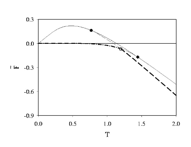
Figure 8: $a=0.5,b=0$. Free energy in the 2-cycle FP scheme for the ML (continuous line), EL/SCL (dashed line) and CR (dash-dot line). We also show $T_{\mathrm{CRE}}(\blacklozenge)$, $T_{\mathrm{M}}(\circ)$ and $T_{\mathrm{MC}}(\bullet).$ Here, as well as in Figures 10 to 12, the stable phases are represented by thick lines while the metastable phases are represented by thin lines.

3.4 2-cycle solution

The phase diagram obtained in the 1-cycle solution scheme cannot be complete because, at low temperatures, ML cannot be the stable phase. At $T=0,$ CR contains an alternating ordered sequence of L and R states in addition to having $l=\frac{1}{2}$ and no O and I states; see Fig. 4. This is a 2-cycle pattern in L and R that is completely missed by the 1-cycle calculation performed above. For ML, $l=\frac{1}{2}$ also, but L and R are statistically distributed. One of these distributions must be the crystal state at $T=0$; indeed, $F_{\mathrm{ML}}(T=0)=F_{\mathrm{CR}}(T=0).$ Despite this, ML immediately above $T=0$ can not represent CR, as it has negative entropy. To obtain the alternating sequence in CR at $T>0$, the above 1-cycle FP scheme is not sufficient to completely describe the physics of the system. We also observe that for $T>0$, there must be local Gujrati-Goldstein excitations [10,11] creating imperfections by local L$\longleftrightarrow$R interchanges in the ordered [..LRLRLR..] sequence. The excitations change a local string LRL into LLL, or RLR into RRR within a square and require 4 bends only. Other excitations, which require (L or R)$\longleftrightarrow$(I or O) on the cactus, can not be done locally and require infinite amount of energy, and need not be considered. This means that the local density $l$ or $r$ will no longer be ${\frac{1}{2}}$. However, if $l>\frac{1}{2}$ at some site, then $r>\frac{1}{2}$ at the next site, followed by $l>\frac{1}{2}$ on the next site and so on.

There are three solutions for the complete system of Eqs. (22)-(27) for any given value of the weights $w$, $w_{\mathrm{p}}$ and $w_{\mathrm{h}}$:

i. A metastable liquid ML (already found in the 1-cycle FP scheme) with:

$l_{\mathrm{a}}=l_{\mathrm{b}}=r_{\mathrm{a}}=r_{\mathrm{b}}=\frac{1}{2}$ and $i_{\mathrm{a}}=i_{\mathrm{b}}=o_{\mathrm{a}}=o_{\mathrm{b}}=0$.

As seen above, this phase represents a liquid phase in which no O and I states are present. The R and L states are randomly distributed in the lattice with the only constraint of having the same number of L and R states at both odd and even layers. This solution exists for any temperature and its free energy has a maximum at $T=T_{\mathrm{K}}\simeq 0.48$.

ii. An equilibrium liquid EL characterized by the presence of all possible states I, O, L and R at both odd and even levels, so that

$l_{\mathrm{a}}=l_{\mathrm{b}}=r_{\mathrm{a}}=r_{\mathrm{b}}=\frac{1}{2}$ and $i_{\mathrm{a}}$, $i_{\mathrm{b}}$, $o_{\mathrm{a}}$, $o_{\mathrm{b}}\neq 0$.

In the 2-cycle solution, $i$ and $o$ on the two sublattices are different, which makes this solution different from the 1-cycle EL solution, in which there is no sublattice structure. Despite this, EL phases in both schemes have identical free energy and various densities. Thus, we no longer make any distinction between the two solutions and identify both of them as the same EL phase. As seen in the previous subsection, the free energy of this phase depends on the value of the parameters $a$ and $b$. This solution exists only for temperatures larger than $T=T_{\mathrm{MC}}(a,b)$.

iii. A crystal phase CR with double degeneracy that is the ground state and that exists for temperatures lower than $T=T_{\mathrm{CRE}}=1/\ln(2)$. The state is perfectly ordered at zero temperature and disorders as the temperature is raised. Fig. 9 shows how the values of $l_{a}$ and $l_{b}$ change with temperature for the CR phase: the two degenerate solutions correspond to a different labeling of the lattice sites where the odd and even levels are just exchanged with each other.

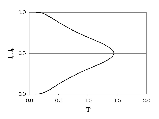
Figure 9: Dependence of $l_{\mathrm{a}}$ and $l_{\mathrm{b}}$ on the temperature for the two phases obtained at low temperature in the 2-cycle fixed point scheme.

The solutions of the system of Eqs. (22)-(27) corresponding to CR and to ML do not depend on the strength of the three- and four- site interaction and, therefore, the free energy curves corresponding to these two phases do not change when the parameters $a$ and $b$ change. In contrast, the free energy of the EL phase depends on the value of $a$ and $b$.

For $a<1$, we have the ground state at $T=0$ in which all the bonds are parallel and there are no bends in the systems. If $a>1$, the four-site interaction becomes more important than the three-site interaction and the ground state at $T=0$ is a step like walk in which there are no parallel bonds and all the sites of the lattice are in a gauche conformation (so that $N_{\mathrm{g}}=N_{\text{S}}$, as said earlier). The two possible ground states are shown in Fig. 4.

4 RESULTS AND DISCUSSION

4.1 Thermodynamic Functions

4.1.1 $b=0$

The complete free energy diagram for $a=0.5$ is given in Fig. 8. The equilibrium phases are represented by the disordered EL at high temperatures and the ordered CR at low temperatures, with a first order transition at a temperature $T_{\mathrm{M}}$ between the two phases, with a discontinuity in the first derivative of the free energy with temperature. This remains true as long as $a>0$. The situation with $a\leq 0$ is different and is discussed later.

The existence of a discontinuous melting temperature for $a>0$ makes it possible to have a supercooled liquid phase through continuation. For $T>T_{\mathrm{M}}$, the EL phase is the stable one. If the liquid phase is cooled in such a way that it is not allowed to undergo the melting transition at $T_{\mathrm{M}}$, then it is possible to have (for $T<T_{\mathrm{M}}$) a supercooled liquid (SCL). The free energy of SCL is obtained by continuing the free energy of the EL phase. This free energy meets critically (i. e. with continuous slopes) with the ML free energy at a temperature that, as before, we call $T_{\mathrm{MC}}$. For $a=0.5$ we find that $T_{\mathrm{MC}}>T_{\mathrm{K}}$, where $T_{\mathrm{K}}$ is the temperature where the ML free energy has its maximum. The critical transition between ML and SCL is a liquid-liquid transition between two liquid phases. As $a$ increases, $T_{\mathrm{MC}}$ moves towards $T_{\mathrm{K}}$. We have observed that for $a\gtrsim 0.8,$ $T_{\mathrm{MC}}<T_{\mathrm{K}}$ (results not shown). In particular, the EL free energy curve itself has a maximum in this case before it merges with the ML curve and, consequently, has an unphysical portion corresponding to the entropy crisis below its maximum.

Figs. 10 and 11 show the entropy and the specific heat vs. temperature, respectively, corresponding to the free energy results shown in Fig. 8. As explained before in the case of the free energy-temperature graphs, the curves corresponding to CR and to ML do not depend on the choice of $a$ and $b$. Table 2 shows how the value of $T_{\mathrm{M}}$ changes as a function of $a$ (in the case $b=0$).

$a$	$T_{\text{M}}$
0	1.443
0.2	1.351
0.5	1.198
0.8	1.009
1	0.878

Table 2: Values of $T_{\mathrm{M}}$ as a function of $a$ (with $b=0$).

Only positive values of $a$ are considered since, as it will be shown below, when the parameter $a$ is negative, there is no first-order melting in the system, provided that $b=0$.

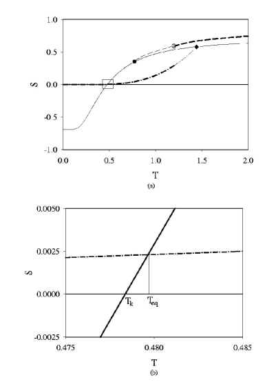
Figure 10: $a=0.5,b=0$. (a) Entropy in the 2-cycle FP scheme for the ML (continuous line), EL/SCL (dashed line) and CR (dash-dot line). We also show $T_{\mathrm{CRE}}(\blacklozenge)$, $T_{\mathrm{M}}(\circ)$ and $T_{\mathrm{MC}}(\bullet)$; (b) magnification of the area contained in the box in (a).

We can calculate the density of gauche bonds $g$ and the density of pairs of parallel bonds $p$ as a function of $T$ and $a$. We can write:

$$g=\partial\omega_{\text{site}}/\partial(\ln(w))|_{w_{\mathrm{p}},w_{\mathrm{h}}},$$ (51)

$$p=\partial\omega_{\text{sq}}/\partial(\ln(w_{\mathrm{p}}))|_{w,w_{\mathrm{h}}},$$ (52)

and calculate the two densities from these derivatives. Note that we have defined the gauche bond density $g$ per site, while the density of parallel bond pairs $p$ is defined per square, since each square contributes one such pair in the ideal CR at absolute zero.

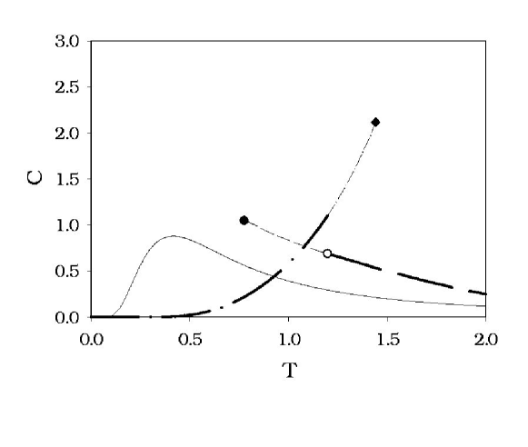
Figure 11: $a=0.5,b=0$. Specific heat in the 2-cycle FP scheme for the ML (continuous line), EL/SCL (dashed line) and CR (dash-dot line). We also show $T_{\mathrm{CRE}}(\blacklozenge)$, $T_{\mathrm{M}}(\circ)$ and $T_{\mathrm{MC}}(\bullet)$.

Fig. 12 shows the gauche bond density and the parallel bond density in the case of $a=0.5$, $b=0$.

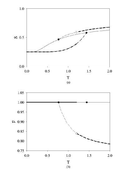
Figure 12: (a) Gauche bond and (b) parallel bond density in the 2-cycle FP scheme for the ML (continuous line), EL/SCL (dashed line) and CR (dash-dot line). We also show $T_{\mathrm{CRE}}(\blacklozenge)$, $T_{\mathrm{M}}(\circ)$ and $T_{\mathrm{MC}}(\bullet)$.

4.1.2 $b\neq 0$

The effect of changing the value of the parameter $b$ is shown in Fig. 13 for $a=0.5$. As we can see, a change in $b$ does not have any effect on the free energy of the CR and ML phases but it does affect the EL phase. Apparently, the effect of $b$ is smaller than the effect of $a$, since the value of the melting temperature does not change significantly as we change $b$. It is worth noting that the presence of the hairpin term alone, even in the absence of the interaction between pairs of parallel bonds, is sufficient to transform the melting transition from second-order, as seen in the case $a=b=0$ (original Flory model), to first-order. If $b$ is negative, the melting and mode-coupling temperatures decrease. If $b$ is positive, instead, these temperatures increase and the melting transition turns into a second-order transition. This is true for any positive value of $b$ in the case $a=0$, while it is true for large enough negative values of $b$ when $a$ is positive.

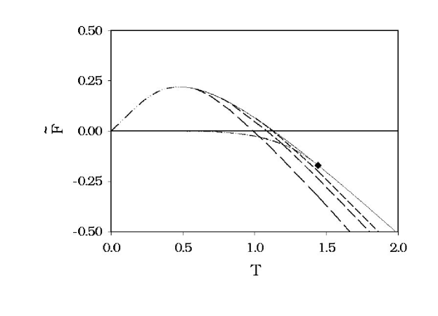
Figure 13: Effect of $b$ on the phase diagram of the system ($a=0.5$). The free energy of ML and CR does not depend on $b$. Three EL/SCL curves are shown corresponding to $b=-0.4$ (long dash), $b=0$ (medium dash) and $b=0.4$ (short dash).

It is interesting to observe that the parallel bond density in ML and in CR is always unity while its value for the EL depends on the temperature.

4.1.3 $a>1$

We consider now the case $a>1$. This case corresponds to a ground state that is not crystalline, as shown in Fig. 4(b). When the four-site interaction is stronger than the three-site interaction, the polymer assumes a configuration that is such that the number of parallel bonds is minimized. In this case there is a very high number of gauche conformations at low temperatures and, even though the polymer assumes an ordered configuration on the lattice, it is not a crystalline configuration according to our definition. Therefore, we do not consider this case any further.

4.1.4 $a<0$

It is also possible to analyze the case in which $a<0$. When $a$ is negative (corresponding to a negative four-site interaction energy $\varepsilon_{\text{p}}$) the temperature $T_{\text{MC}}$ at which the EL appears moves to higher values. Since the temperature $T_{\text{M}}(\equiv T_{\text{CRE}})$ at which CR appears is unaffected by the choice of the value of $a$, a shift of the origin of the EL phase to higher temperatures makes ML the equilibrium phase for temperatures between $T_{\text{M}}$ and $T_{\text{MC}}>T_{\text{M}}$; it is no longer a metastable phase in this range. We identify the equilibrium portion of the ML phase as a new equilibrium phase, and denote it by EL${}_{\text{ML}}$; the subscript is a reminder that the phase is associated with the ML phase. The new phase is again a liquid phase. Hence, the transition at $T_{\text{MC}}$ is a liquid -liquid transition and is continuous. Similarly, the transition at $T_{\text{M}}$ between CR and EL${}_{\text{ML}}$ is also a continuous transition. Since ML exists below $T_{\text{M}}$, we can formally treat the ML phase below $T_{\text{M}}$ as obtained by continuation of EL${}_{\text{ML}}$ below $T_{\text{M}}$, but this continuation should not be taken as a supercooled liquid below $T_{\text{M}}$, as there will be no energy barrier due to the continuous melting transition. Furthermore, since the liquid-liquid transition at $T_{\text{MC}}$ occurs at a temperature higher than the melting temperature, this case has no relevance for studying the glass transition. Hence, we do not pursue it further. The same behavior is observed, as explained above, when $a=0$ and $b>0$.

4.1.5 Choice of $a$

Because of the above considerations, we consider $a$ in the range 0 $<$$a$ $<$1. In this range, the four-site interaction is repulsive (the system spends some energy to align two segments parallel to each other) and the ground state is the crystalline one [see Fig. 4(a)]. In this case, the model exhibits a first order melting transition at a temperature $T_{\text{M}}=T_{\text{M}}(a)$ between EL, that is stable at temperatures higher than $T_{\text{M}}$, and CR, that is stable for temperatures lower than $T_{\text{M}}$. It can be observed that the discontinuity in the specific heat at $T_{\text{MC}}$ is a function of the parameters $a$ and $b$. In particular, if we fix $b$, as $a$ increases the discontinuity gets smaller and smaller as long as $a$ $<$0.8, and then starts growing again while the transition temperature keeps moving to lower values; the results are not shown.

The crystalline phase is an ordered one but, unlike the ground state predicted by the original Flory model [1,2] (Fig. 1), it has non zero entropy. It also satisfies the Gujrati-Goldstein bounds. The I and O states disappear in the crystalline phase but this phase has non zero entropy because of the many possible configurations that the polymer chain can assume corresponding to different sequences of L and R states. The entropy of the crystalline phase goes to zero only when the temperature goes to zero, which is consistent with the third law of thermodynamics.

If the cooling process is such that the system can avoid crystallization at $T_{\text{M}}$, the equilibrium liquid EL can be supercooled to give rise to SCL that transforms into the metastable liquid ML through a liquid-liquid second-order transition at $T_{\text{MC}}\leq T_{\text{M}}$ (no latent heat is associated with the transition). The metastable liquid and the equilibrium liquid phases are somehow similar. The metastable liquid consists of a random sequence of R and L states, while the equilibrium liquid consists of a random sequence of R, L, I and O states. The presence of O and I states makes the total energy and the entropy of the equilibrium liquid larger than those of the metastable liquid, see Figs. 10 and 11.

4.2 Relation with the Mode-coupling Transition

We tentatively identify the critical temperature $T_{\text{MC}}$ of the liquid-liquid transition as the mode-coupling transition temperature because the transition exhibits some of the features predicted by the original mode coupling theory at the critical mode-coupling transition temperature. It should be remarked that our equilibrium investigation cannot provide any direct information about the dynamics at $T_{\text{MC}}$ except by inference. Hence, the connection we allude to above should only be taken as tentative, in view of the fact that the mode-coupling transition, applied successfully to simple fluids, is considered to be a dynamic transition. We can only add that the mode-coupling theory is not well-understood for long polymers, and it is not clear what its predictions might be for infinite polymers that we are investigating here.

According to this theory, the dynamics slows down according to Eq. (3) near $T_{\text{MC}}.$ The local molecular structure freezes and only long-time cooperative jumps are allowed below this temperature. Thus, the dynamic transition is between two disordered states, very much like the thermodynamic liquid-liquid transition we observe in our calculation. Let us consider the behavior of the correlation length $\xi_{\text{SCL}}$ of the system near the critical temperature $T_{\text{MC}}$. As $T_{\text{MC}}$ is approached from above $(T\rightarrow T_{\text{MC}}^{+}),$ the correlation length $\xi_{\text{SCL}}$ of the supercooled liquid must diverge to infinity because the transition is continuous. It is very easy to observe from the results that there is a discontinuity in the specific heat of the system at the transition from the supercooled liquid to the metastable liquid. Indeed, the SCL terminates at $T_{\text{MC}}$ as $T\rightarrow T_{\text{MC}}^{+}.$ The disappearance of SCL is what gives rise to this divergence, which will contribute to the critical slowing down of the system. Such a critical slowing down is exhibited at the mode-coupling transition [39]; see Eq. (3).

On the other hand, ML exists at all temperatures. Thus, there would be no divergence at $T_{\text{MC}}$ in the correlation length $\xi_{\text{ML}}$ associated with ML . Indeed, its specific heat remains continuous. This will imply that the dynamics of the system should not undergo any significant change at the critical temperature $T_{\text{MC}}$ if we approach it while heating up ML in such a way that ML is not allowed to turn into SCL. In simulation, one can investigate ML by suppressing fast relaxations that are supposed to freeze at the mode-coupling temperature. Such an attempt has already been made [25] where one sees no anomalous behavior at the mode-coupling temperature. Parisi and coworkers [25] while analyzing a Lennard-Jones system have observed this kind of dynamics. In their approach, the fast dynamics of the system (the one pertinent to the supercooled liquid in our model) is suppressed and only the slow dynamics of the system is taken into account. The slow dynamics is described as a relaxation process taking place in a connected network of potential energy minima. Indeed, the authors only observes an Arrhenius behavior in the relaxation time, as opposed to the Vogel-Tammann-Fulcher behavior associated with the mode-coupling transition. Even though the system studied by Parisi and coworkers is very different from the polymer system studied here, it is important to note that all the numerical results obtained in the case of the Lennard-Jones fluid are in agreement with the experimental findings in non-network forming glasses and especially in glasses that are fragile according to Angell’s definition [40].

Recent experimental results obtained by Sokolov and coworkers [41] studying polyisobutylene and polystyrene show the presence of a critical behavior only above $T_{\text{MC}}$ along with the failure of the predictions of the mode coupling theory below the critical temperature. These authors show many similarities between the results obtained on these polymeric glasses and the ideas of the liquid-liquid transition in polymeric liquids formulated by Boyer and coworkers [42,43]. It is worth noting that this liquid-liquid transition would manifest itself through a discontinuity in the first derivative of the specific heat (and not the specific heat itself as in the present case) at the transition temperature. This makes Boyer’s result very different from our result. The idea introduced by Boyer has been strongly criticized and is still the subject of discussion [44,45].

The second similarity has to do with our choice of the parameter $a$, so that $T_{\text{MC}}$ lies above the Kauzmann temperature $T_{\text{K}}.$ This is also what is expected in the mode-coupling theory in which the transition occurs above the conventional glass transition temperature.

The third similarity appears when we allow free volume in our model in Eq. 9(b), as has been done recently [29]. It is found that the free volume in the model for the case of infinite polymers vanishes identically at $T_{\text{MC}}$, and remains zero below it. Consequently, one expects the viscosity to diverge at $T_{\text{MC}}$.

While the mode coupling theory describes the transition at $T_{\text{MC}}$ as dynamic in nature, our results show that the transition at $T_{\text{MC}}$ is thermodynamic in nature. The sharp transition is due to the polymer being infinitely long, and disappears as soon as polymers become finite in size [29]. However, for polymers of reasonable sizes, there will continue to be a narrow crossover region between two phases (ML and SCL).

4.3 Ground State and Kauzmann Temperature

Below $T_{\text{MC}}$, the only two phases that are present are the metastable liquid and the crystal. Above $T_{\text{MC}}$, the supercooled liquid, which is the continuation of the equilibrium liquid above $T_{\text{M}}$, is more stable than the metastable liquid and coexists with the crystal. It is worth noting that the modified free energies $\widetilde{F}$ of both the metastable liquid and the supercooled liquid cross over and becomes positive at some finite and non-zero temperature. Let us focus on the metastable liquid as its behavior is easy to describe since its modified free energy $\widetilde{F}$  remains independent of$\ a$ and $b$. We first observe that the 2-cycle FP solution contains within its possible solutions the 1-cycle solution. We also find that the free energy of all possible 2-cycle solutions (including the 1-cycle solutions) at absolute zero are the same: $\widetilde{F}=0.$

Because of the exact nature of our calculation, this equality of the ML and CR free energies at absolute zero is not brought about due to any approximation. Because of this equality at absolute zero, we will now consider the modified free energy $\widetilde{F}$ in the following. The CR free energy remains negative at all temperatures and approaches zero at absolute zero. Thus, CR has non-negative entropy. On the other hand, the ML free energy $\widetilde{F}$, which is negative at higher temperatures, becomes positive at some intermediate and non-zero temperature $T_{\text{M0}}$ and keeps increasing, as the temperature is lowered, until the Kauzmann temperature $T_{\text{K}}$ ($\approx 0.48$ in our model) is reached. Below $T_{\text{K}}$, the ML free energy $\widetilde{F}$  must necessarily decrease since it must vanish at absolute zero. The maximum of $\widetilde{F}$ corresponds to the vanishing of the entropy of the ML phase, below which the entropy must become negative [46]. Thus, the existence of the Kauzmann temperature is a consequence of the fact that the ML free energy $\widetilde{F}$ , once it crosses the zero at $T_{\text{M0}}$, must necessarily decrease at some lower temperature so as to return to zero at absolute zero. The existence of the maximum in $\widetilde{F}_{\text{ML}}$ as a function of  the temperature is the root of the rapid entropy drop noted by Kauzmann [5]. The maximum at a positive $T_{\text{K}}$ is forced by thermodynamics since the larger specific heat of ML makes $\widetilde{F}_{\text{ML}}$ cross over to positive values at $T_{\text{M0}}$. If we had carried out our calculation in some approximation, as is the case with the calculation of Gibbs and DiMarzio [8], we certainly could not draw this remarkable conclusion.

4.4 $\mathit{S}_{\text{CR}}\mathbf{>}\mathit{S}_{\text{SCL}}$ and Entropy Crisis

The crystalline phase has an entropy that is never negative. Hence, its entropy is larger than the entropy of the metastable liquid in the temperature interval $T_{\text{K}}<T<T_{\text{eq}}$, where $T_{\text{eq}}$ is the temperature at which the entropy of the two phases is the same (see Fig. 10(b)). This result contrasts the common belief [17] that the entropy of a crystalline phase must always be lower than the entropy of the corresponding liquid phase, even if the latter is an equilibrium phase. Our results clearly show that there is no thermodynamic requirement for this belief to be true. Indeed, real systems like He conform with this observation.

In order to sustain the common belief that the entropy of the liquid must always be larger than that of the crystal, it was conjectured by Kauzmann that the system must avoid the (Kauzmann) catastrophe caused as soon as the requirement $S_{\text{CR}}\leq S_{\text{SCL}}$ is violated. The system is supposed to avoid the catastrophe by undergoing either a spontaneous crystallization, as proposed by Kauzmann in his original paper, or an ideal glass transition [5,8,15,47].

The most important result of the present research regarding the Kauzmann catastrophe is that since our calculations show that it is possible to observe $S_{\text{CR}}>S_{\text{SCL}}$ in an explicit model calculation, the existence of the catastrophe must be reinterpreted in terms of the entropy crisis corresponding to having no realizable state (negative entropy) [46]: the catastrophe happens at a temperature $T_{\text{K}}$ where the entropy of the metastable liquid goes to zero and not at the temperature $T_{\text{eq}}$ at which the entropy of the liquid becomes equal to the entropy of the crystal. The two temperatures coincide in the original Flory model since the entropy of the crystal is identically equal to zero below $T_{\text{M}}$, see Fig. 1, while in our exact calculation, the two temperatures are different because the entropy of the crystal is zero only when the temperature goes to zero.

4.5 Ideal Glass Transition

The ML free energy has no physical relevance below $T_{\text{K}}$ since it corresponds to negative values of the entropy. Decreasing the temperature as $T\rightarrow T_{\text{K}}^{+}$ the entropy falls very rapidly to zero (as seen, for example, in Fig. 10 (b)). As the temperature is decreased, the energy of the metastable liquid cannot increase because this would correspond to a negative specific heat. At the same time, this energy cannot decrease since there are no states with non-negative entropy (except the crystal phase, but we do not consider this possibility here) available to the system. The only conclusion that can be drawn from these observations is that for $T<T_{\text{K}}$, the metastable liquid remains frozen in the state in which it finds itself at $T_{\text{K}}$. This describes the ideal glass transition. In our analysis, ML does not undergo any changes in its state at the glass transition, so that this transition cannot be a first-order transition as recently proposed by Parisi and coworkers [26(b)].

It is interesting to notice that the energy of the metastable liquid increases monotonically with $T$ and is very similar to the excitation profiles for other systems like the mixed Lennard-Jones system [48] and the two states model [49].

It is also interesting to notice that our model predicts, at the Kauzmann temperature, an upward discontinuity for the specific heat. The specific heat of the metastable liquid is decreasing with the temperature for $T>T_{\text{K}}$. This kind of behavior is in disagreement with many experimental results but has been observed in computer simulations by Parisi and coworkers [26] and experimentally (at least in some temperature interval immediately above the glass transition) in glasses formed by low molecular weight materials of very different nature like 1-butene [45] and the metallic system Au-Si [40].

4.6 Flory Model

The value $a=1$ corresponds to a borderline case. As we have shown in Fig. 4, if $a$ is larger than 1 then the ground state is not crystalline anymore and there are no parallel bonds at $T=0$. Correspondingly, we observe from our results that as $a\rightarrow 1$, $T_{\text{MC}}$ moves to lower and lower values and eventually goes to zero when $a$ goes to one. We also find that, if we keep $b$ fixed, then as the value of $a$ increases, the values of $T_{\text{M}}$ and $T_{\text{MC}}$ decrease and, as said above, for $a\geq 0.8$, the supercooled liquid shows its own Kauzmann temperature corresponding to the maximum in its free energy. If $a$ becomes negative, the critical temperature moves to higher temperatures. Unlike the case of $a>0$, there is a temperature interval $(T_{\text{M}}<T<T_{\text{MC}})$ where the metastable liquid becomes the stable phase EL${}_{\text{ML}}$. The melting transition that is observed is a continuous transition. This aspect is in disagreement with experimental observations.

If $a=b=0$, as explained before, the model reduces to the Flory model of polymer melting. In this case $T_{\text{M}}=T_{\text{MC}}=T_{\text{CRE}}$ and the melting transition from the equilibrium liquid to the crystalline phase becomes continuous in contrast with the original calculations of Flory. It is important to notice that in this case there is no possibility to obtain a supercooled liquid since the equilibrium liquid phase disappears continuously into the crystal at $T_{\text{M}}$.

The solution found by Flory for the original model corresponds to a tricritical solution: if we consider the melting transition present in the system, this transition is first order for $a>0$ and continuous for $a<0$. In the latter case, we have $T_{\text{M}}\equiv T_{\text{CRE}}$, as shown in Fig. 14.

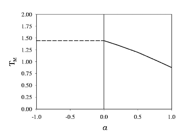
Figure 14: Dependence of the melting temperature on $a$. The first-order transition line (continuous line ) and the second-order transition line (dashed line) are shown.

It seems reasonable to assume that in order to be able to describe the physics of real systems, the value of the parameter $a$ must be chosen in the range between 0 and 0.7 while the value of $b$ should be in the range $-0.5-0.5$.

4.7 Comparison with A Real System

By a proper choice of various parameters in our model, we can fit the predictions of our theory with experiments. We discuss one such example below. Setting $a=0.5$ and $b=0$, for example, our model predicts $T_{\text{M}}/T_{\text{k}}\simeq 1.20/0.48$. We can consider polyethylene (PE) and try to describe its thermodynamic properties using our model. The experimentally measured melting temperature of PE is $T_{\text{M}}($PE$)\simeq 400$K. Then the model predicts $T_{\text{K}}($PE$)\simeq 160$K. This temperature is about 40K below the experimentally determined glass transition. Since we expect the experimental glass transition to occur above the ideal glass transition because of experimental constraints, we can conclude that the prediction of our model is, at least, reasonable.

5 CONCLUSIONS

We have considered an extension of the Flory model of melting by introducing two additional interactions characterized by parameters $a$ and $b$. One interaction is between a pair of parallel bonds and the second one is due to a hairpin turn. The model is defined on a checkerboard version of the square lattice, and has been solved exactly on a Husimi cactus, which is a recursive lattice [36]. It should be recalled [36] that calculations done on a recursive lattice have been shown to be more reliable than conventional mean-field calculations. The choice of the Husimi cactus is also important for the inclusion of the Gujrati-Goldstein excitations that are responsible for destroying the complete order in the crystal phase CR [10-12] in the Flory model. The method of calculation is to look for the fix-point (FP) solution of the recursion relations. We need to consider 1-cycle and 2-cycle FP solutions to describe the disordered phase and the crystal phase, respectively. This has required us to provide in this work the extension of the Gujrati trick [36] to calculate the free energy of the 1-cycle FP solution to the 2-cycle solution. The exact nature of the solution allows us to draw some important conclusions, which would not have been drawn with the same force, had we obtained the solution under ambiguous and/or uncontrollable approximations.

We have identified an equilibrium liquid phase EL at high temperatures $T\geq T_{\text{M}}$. There is another liquid phase ML which exists at all temperatures, but which never becomes an equilibrium phase for appropriate choices of the parameters $a$ and $b$. Below the melting temperature $T_{\text{M}}$, the crystal phase CR becomes the equilibrium phase. The melting transition is usually a first order transition with a latent heat, below which we can continue EL to give rise to the supercooled liquid phase SCL. This phase terminates at a lower temperature $T_{\text{MC}}$, where it meets ML continuously with no latent heat. The transition at $T_{\text{MC}}$ is a continuous liquid-liquid transition.

Both SCL and ML represent metastable phases in the system. For a metastable state to exist in Nature, its entropy must be non-negative. A negative entropy ($S<0)$ in metastable states (SCL and/or ML) implies that such states cannot exist. We have argued that the ML free energy must have a maximum at $T_{\text{K}}$ as a function of the temperature $T$; see Fig. 8. Thus, ML has non-negative entropy above $T_{\text{K}}$, but gives rise to negative entropy below $T_{\text{K}}$. We have called the appearance of $S<0$ the entropy crisis , which we have used instead of the Kauzmann paradox ($S_{\text{ML}}<S_{\text{CR}}$) as the driving force behind the ideal glass transition at $T_{\text{K}}$. The ideal glass transition occurs in the metastable liquid ML, and not in SCL, which is contrary to the conventional wisdom. The portion of ML below $T_{\text{K}}$ must be replaced by the ideal glass (see dotted thin horizontal portion below $T_{\text{K}}$ in Fig. 8), which is completely inactive in that its entropy and specific heat are both zero. The rapid drop in the entropy near the Kauzmann temperature $T_{\text{K}}$ is a direct consequence of the existence of the maximum in the ML free energy. The liquid-liquid transition at $T_{\text{MC}}$ between the two metastable phases ML and SCL has been shown to share many similarities with the critical mode-coupling transition, even though the latter is known to be driven by dynamics in simple fluids. It should be remarked that nothing is known about this dynamic transition in the semiflexible Hamilton walk limit of infinite polymers.

The Flory model is shown to give rise to a continuous melting. Indeed, the melting point in the Flory model turns out to be a tricritical point in our calculation. It would be interesting to see if this conclusion can be sustained in other computational scheme.

The natural extension of this model in Eq. (9b) involves the analysis of the effects of compressibility (taking into account voids as another species on the lattice) and of finite chain size, both in the polydisperse and in the monodisperse case. This is reported elsewhere [29,30].

We finally discuss an interesting aspect of the 2-cycle FP solution  for EL/SCL observed by Semerianov [50]. The values of $i_{\mathrm{a}}$, $i_{\mathrm{b}}$, $o_{\mathrm{a}}$, and $o_{\mathrm{b}}$ depend on the choice of the initial guesses used in the FP solution of the recursion relations. Thus, there are many different 2-cycle solutions for EL/SCL that differ in the values of $i_{\mathrm{a}}$, $i_{\mathrm{b}}$, $o_{\mathrm{a}}$, and $o_{\mathrm{b}}.$What we find is that the product $io$ remains the same on both sublattices for all initial guesses, and that they all give the same free energy and densities. We hope that the observation will provide some useful information about the free energy landscape picture, but this requires further investigation. We hope to report on this in near future.

ACKNOWLEDGEMENTS

We would like to thank Sagar Rane and Fedor Semerianov for fruitful discussions.

APPENDIX

We index the cactus levels in a slightly different manner here for simplicity. If the base site of a square is indexed $m$, then the intermediate and the peak sites are all indexed $m+1$. The square is still called the $m$th square. The origin is indexed, as before, $m=0$. We evaluate $N_{(m)}$, the number of sites at the $m$th generation of a tree rooted at the origin ($m=0$). The rooted tree is only half of a complete tree. It is evidently given by:

$$N_{(m)}=3^{m},$$

so that the total number of sites belonging to the first $m$ generations (and excluding the origin) of a rooted tree is:

$$N_{(m)}^{rooted}=\overset{m}{\underset{k=1}{\sum}}N_{(k)}=\frac{3^{m+1}-3}{2}.$$

The total number of sites belonging to the first $m$ generations of the complete tree is then equal to twice the total number of sites belonging to the first $m$ generations of a rooted tree plus one since we have to consider the origin too:

$$\widetilde{N}_{m}=2N_{(m)}^{rooted}+1=3^{m+1}-2.$$

Let us consider now the number $S_{(m)}$ of the$\ m$th generation squares ($m\geq 0$) of the rooted tree. Clearly we have:

$$S_{(m)}=3^{m}.$$

The total number of squares belonging to the first $m$ generations of a rooted tree (so that the maximum generation of the squares is $m-1$) is:

$$S_{(m)}^{rooted}=\overset{m-1}{\underset{k=0}{\sum}}S_{(k)}=\frac{3^{m}-1}{2}.$$

The total number of squares belonging to the first $m$ generations of the complete tree is then just twice the total number of squares belonging to the first $m$ generations of a rooted tree:

$$\widetilde{S}_{m}=2S_{(m)}^{rooted}=3^{m}-1.$$

In order to make the cactus homogeneous, we must consider it to be part of a larger cactus. Consequently, both $\widetilde{S}_{m}$ and $\widetilde{N}_{m}$ must be modified in order to take into account the presence of dangling bonds at surface sites: we consider to add half a square to each surface site. Recalling that each square contains four half-sites (a site is shared by two squares), we conclude that each square contributes two sites to the number of sites. Hence, each half-square contributes one site to the site count. Thus, we modify $\widetilde{N}_{m}$ by adding 1 site for each surface square. This gives for the total number of sites

$$N_{m}=\widetilde{N}_{m}+3^{m}=4\times 3^{m}-2.$$

Modifying $\widetilde{S}_{m-1}$ by the half-squares at the surface sites gives for the total number of squares:

$$S_{m}=\widetilde{S}_{m-1}+\frac{1}{2}\times 2\times N_{(m)}=2\times 3^{m}-1.$$

Now, if we consider the thermodynamic limit in which $m\rightarrow\infty$ we have:

$$\frac{S_{m}}{N_{m}}\rightarrow\frac{1}{2}.$$

which is consistent with our earlier homogeneous hypothesis $N_{\text{S}}=N$  relating the total number of squares $N_{\text{S}}$ and the total number of sites $N$.

Let us finally consider the total number $\widetilde{B}_{m}$ of bonds in the first $m$ generations ($m>0$)  of the tree. Each square contains four bonds, and there are $\widetilde{S}_{m}$ squares in this tree. Thus

$$\widetilde{B}_{m}=4(3^{m}-1).$$

The modification of the lattice introduced above implies that we must now add half-square at each of the surface sites of the $m$th generations ($m>0$) tree. Each half-square contributes 2 bonds. Hence

$$B_{m}=\widetilde{B}_{m}+4\times 3^{m}=8\times 3^{m}-2.$$

If we consider the thermodynamic limit in which $m\rightarrow\infty$ we have:

$$\frac{B_{m}}{S_{m}}\rightarrow 4,$$

as expected.

References

- [1] P. J. Flory, J. Chem. Phys. 10, 51 (1942).
- [2] P. J. Flory, Proc. R. Soc. A234, 60 (1956).
- [3] J. F. Nagle, P. D. Gujrati and M. Goldstein, J. Phys. Chem. 88, 4599 (1984).
- [4] M. L. Huggins, Ann. N. Y. Acad. Sci. 41, 1 (1942).
- [5] W. Kauzmann, Chem. Rev. 43, 219 (1948).
- [6] J. Jäckle, Rep. Prog. Phys. 49, 171 (1986).
- [7] P. G. Debenedetti, Metastable Liquids, Concepts and Principles (Priceton University Press, Princeton, N. J., 1996).
- [8] J. H. Gibbs and E. A. DiMarzio, J. Chem. Phys. 28, 373 (1958); 28, 807 (1958); J. Polymer Sci. 40, 121 (1963); G. Adams and J. H. Gibbs, J. Chem. Phys. 43, 139 (1965).
- [9] The Glass Transition and the Nature of the Glassy State, edited by M. Goldstein and R. Simha (Ann. N.Y. Acad. Sci., New York, 1976).
- [10] (a) P. D. Gujrati, J. Phys. A13, L437 (1980); (b) P. D. Gujrati and M. Goldstein, J. Chem. Phys. 74, 2596 (1981).
- [11] P. D. Gujrati, J. Stat. Phys. 28, 241 (1982).
- [12] (a) R. G. Petschek, Phys. Rev. B32, 474 (1985); (b) A. Baumgartner, D. Y. Yoon, J. Chem. Phys. 79, 521 (1983).
- [13] J. Suzuki and T. Izuyama, J. Phys. Soc (Japan) 57, 818 (1988).
- [14] F. H. Stillinger, J. Chem. Phys. 88, 7818 (1988).
- [15] C. A. Angell, J. Non-Cryst. Solids 131-133, 13 (1991).
- [16] D. Kivelson, S. A. Kivelson, X. Zhao, Z. Nussinov, and G. Tarjus, Physica A 219, 27 (1995).
- [17] See articles in J. Res. NIST 102, No. 2 (1997).
- [18] G. P. Johari, J. Chem. Phys. 113, 751 (2000).
- [19] F. H. Stillinger, P. G. Debenedetti, and T. M. Truskett, J. Phys. Chem. B 105, 11809 (2001).
- [20] W. Göetze, in Liquids, Freezing and the Glass Transition, edited by J. P. Hansen and D. Levesque (Plenum, New York, 1989).
- [21] U. Bengtzelius, W. Göetze and A. Sjölander, J. Chem. Phys. 77, 5915 (1984); C. A. Angell, L. Monnerie and L. M. Torell, Symp. Mater. Res. Soc. 215, 3 (1991).
- [22] W. Göetze and A. Sjölander, Rep. Prog. Phys. 55, 241 (1992).
- [23] D. J. Plazek and K. L. Ngai, Macromolecules 24, 1222 (1991).
- [24] S. Franz and G. Parisi, Phys. Rev. Lett. 79, 2486 (1997).
- [25] L. Angelani, G. Parisi, G. Ruocco and G. Viliani, Phys Rev. Lett. 81, 4648 (1998); Phys. Rev. E 61, 1681 (2000).
- [26] M. Mezard and G. Parisi, Phys. Rev. Lett. 82, 747 (1999); B. Coluzzi, G. Parisi and P. Verrocchio, Phys. Rev. Lett. 84, 306 (2000).
- [27] G. I. Menon and R. Pandit, Phys. Rev. E 59, 787 (1999).
- [28] P. D. Gujrati, and A. Corsi, Phys. Rev. Lett. 87, 025701 (2001).
- [29] P. D. Gujrati, S. S. Rane, and A. Corsi, Phys. Rev. E 67, 052501 (2003).
- [30] S. S. Rane, and P. D. Gujrati, submitted for publication.
- [31] (a) P. D. Gujrati, submitted for publication; (b) P. D. Gujrati and F. Semerianov, to be published.
- [32] In classical statistical mechanics, which is what is conventionally used to analyze metastability, the contribution to the total entropy from the translational degrees of freedom is the same for various possible phases like SCL or CR that can exist at a given temperature, and is a function only of the temperature . This is because the kinetic energy is decoupled from the interaction energy in classical mechanics, making the translational degrees of freedom decouple from the rest [31(a)]. Thus, the translational degrees of freedom do not have to be considered in the investigation. The difference can be equally well used to characterize various phases of the system; it is known as the configurational entropy of the system and determines the configurational partition function. In lattice models like the one considered here, we do not have the translational degrees of freedom, and the translational entropy is zero. Hence, there is no distinction between the total entropy and the configurational entropy in lattice models. For this reason, we will not use the subscript ”conf” to denote the configurational entropy in this work.
- [33] M. Mezard, G. Parisi and M. A. Virasoro, Spin Glass Theory and Beyond (World Scientific, Singapore, 1987).
- [34] R. B. Griffiths and P. D. Gujrati, J. Stat. Phys. 30, 563 (1983).
- [35] P. D. Gujrati, Phys. Rev. B 32, 3319 (1985).
- [36] P. D. Gujrati, Phys. Rev. Lett. 74, 809 (1995).
- [37] (a) P. D. Gujrati, Phys. Rev. A 24, 2096 (1981); (b) P. D. Gujrati, J. Chem. Phys. 98, 1613 (1993).
- [38] See for example, H. W. Blote and B. Nienhuis, Phys. Rev. Lett. 72, 1372 (1994); M. T. Batchelor, J. Suzuki, and C. M. Yung, Phys. Rev. Lett. 73, 2646 (1994); J. Kondev and J. L. Jacobsen, Phys. Rev. Lett. 81, 2922 (1998).
- [39] K. Kawasaki, Ann. Phys. 61, 1 (1970).
- [40] C. A. Angell, Science 267, 1924 (1995).
- [41] A. Kisliuk,. R.T. Mathers and A. P. Sokolov, J. Poly. Sci.: Pol. Physics 38, 2785 (2000).
- [42] R. F. Boyer, Pol. Eng. Sci. 19, 732 (1979); R. F. Boyer and R. L. Miller, Macromolecules 17, 365 (1984).
- [43] S. S. N. Murthy, J. Poly. Sci.: Pol. Physics 31, 475 (1993).
- [44] D. J. Plazek, J. Poly. Sci.: Pol. Physics 20, 1533 (1982).
- [45] O. Yamamuro, S. Takahara, A. Inaba, T. Matsuo and H. Suga, J. Phys. Cond. Matt. 6, L169 (1994).
- [46] It should be stressed at this point that the existence of a negative entropy in our exact calculation is caused by the use of the continuation and/or the use of solutions that are not the equilibrium one, i.e. solutions that do not have the lowest possible free energy Recall that the exact calculation of the free energy through the use of the partition function only requires that the free energy have the correct convexity property, which in this case corresponds to having a non-negative specific heat. This remains true of all states in our calculation, equilibrium or not. The requirement that the entropy be non-negative is an additional postulate, justified by the obvious fact that the number of realizable configurations be at least one. The continuation need not satisfy the entropy requirement, the latter being completely independent of the convexity property of the free energy. There will never be a negative-entropy equilibrium solution in any exact calculation, as the equilibrium state must correspond to a number of realizable configurations. This also means that if there is no phase transition in a model, there will be no possibility of any continuation that can then violate the entropy requirement. In this case, there cannot exist any Kauzmann temperature.
- [47] M. Goldstein, J. Chem. Phys. 51, 3728 (1969).
- [48] S. Sastry, P. G. Debenedetti and F. H. Stillinger, Nature 393, 554 (1998).
- [49] C. A. Angell, B. E. Richards and V. Velikov, J. Phys. Cond. Matt. 11, A75 (1999).
- [50] F. Semerianov, private communication.