Noise reduction in chaotic time series by a local projection with nonlinear constraints

Abstract

On the basis of a local-projective (LP) approach we develop a method of noise reduction in time series that makes use of nonlinear constraints appearing due to the deterministic character of the underlying dynamical system. The Delaunay triangulation approach is used to find the optimal nearest neighboring points in time series. The efficiency of our method is comparable to standard LP methods but our method is more robust to the input parameter estimation. The approach has been successfully applied for separating a signal from noise in the chaotic Henon and Lorenz models as well as for noisy experimental data obtained from an electronic Chua circuit. The method works properly for a mixture of additive and dynamical noise and can be used for the noise-level detection.

I Introduction

It is common that observed data are contaminated by noise (for a review of methods of nonlinear time series analysis see kantzschreiber ; abarbanel ; kapitaniak ). The presence of noise can substantially affect such system parameters as dimension, entropy or Lyapunov exponents urbanowicz . In fact noise can completely obscure or even destroy the fractal structure of a chaotic attractor kostelich and even $2\%$ of noise can make a dimension calculation misleading Schreiber1 . It follows that both from the theoretical as well as from the practical point of view it is desirable to reduce the noise level. Thanks to noise reduction kostelich ; Schreiber2 ; Farmer ; hammel ; davies ; zhang ; chen ; Grassberger ; kalman ; effern ; Hsu ; Sauer ; Schreiber it is possible e.g. to restore the hidden structure of an attractor which is smeared out by noise, as well as to improve the quality of predictions.

Every method of noise reduction assumes that it is possible to distinguish between noise and a clean signal on the basis of some objective criteria. Conventional methods such as linear filters use a power spectrum for this purpose. Low pass filters assume that a clean signal has some typical low frequency, respectively it is true for high pass filters. It follows that these methods are convenient for a regular source which generates a periodic or a quasi-periodic signal. In the case of chaotic signals linear filters cannot be used for noise reduction without a substantial disturbance of the clean signal. The reason is the broad-band spectrum of chaotic signals. It follows that for chaotic systems we make use of another generic feature of dissipative motion located on attractors that are smooth submanifolds of an admissible phase space. As results corresponding state vectors reconstructed from time delay variables are limited to geometric objects that can be locally linearized. This fact is a common background of all local projective (LP) methods of noise reduction.

Besides the LP approach there are also noise reduction methods that approximate an unknown equation of motion and use it to find corrections to state vectors. Such methods make use of neural networks zhang or a genetic programming chen and one has to assume some basis functions e.g. radial basis functions broomhead to reconstruct the equation of motion. Another group of methods are modified linear filters e.g. the Wiener filter Grassberger , the Kalman filter kalman , or methods based on wavelet analysis effern . Applications of these methods are limited to systems with large sampling frequencies, and they are confined to the neighborhood of every point in phase space.

The method described in this paper can be considered as an extension of LP methods by taking into account constraints that occur due to the local linearization of the equation of motion of the system. We call our method the local projection with nonlinear constraints (LPNC).

The paper is organized as follows. In the following section we shall present the general background of LP methods. The LPNC method is introduced in Sec. III and compared with LP methods in Sec. IV. In Sec. V we present methods how to find the nearest neighborhood, and examples of noise reduction and estimation are introduced in Secs. VI and VII. In the appendix A one can find the multidimensional generalization of the solution presented in Sec. III.

II Local Projective Methods of Noise Reduction

Let us consider a scalar time series $\{\tilde{x}_{n}\}$, $n=1,2,...,N$ corresponding to an experimentally accessible component of the system trajectory. We assume that in the presence of measurement noise instead of the clean time series $\tilde{x}_{n}$ we observe a noisy series $x_{n}$: $x_{n}=\tilde{x}_{n}+\eta_{n}$ where $\eta_{n}$ is the noise variable. The aim of noise reduction methods is to estimate the set $\{\tilde{x}_{n}\}$ from the observed noisy data set $\{x_{n}\}$, i.e. to find corrections $\delta x_{n}$ such that $x_{n}+\delta{x}_{n}\approx\tilde{x}_{n}$. The corrections $\delta x_{n}$ can be estimated on the assumption that $\tilde{x}_{n}$ belongs to a clean deterministic trajectory. Let us create vectors of the system state $\tilde{\mathbf{x}}_{n}$ using the Takens Theorem abarbanel $\tilde{\mathbf{x}}_{n}=\{\tilde{x}_{n},\tilde{x}_{n-\tau},...,\tilde{x}_{n-(d-1)\tau}\}$, where $d$ is the embedding dimension, and $\tau$ is the embedding delay that further will be just $1$. Now the simple approach is to use a linear approximation for the nearest neighborhood $\tilde{\mathbf{X}}_{n}^{NN}$ of a vector $\tilde{\mathbf{x}}_{n}$ and then to estimate an unknown equation of motion in the embedded space by a linear fit: $\tilde{\mathbf{x}}_{n+1}=\mathbf{A}\tilde{\mathbf{x}}_{n}+\mathbf{b}$. The matrix $\mathbf{A}$ is the corresponding Jacobi matrix and $\mathbf{b}$ is a constant vector.

In LP methods the local linearity of the system dynamics plays the crucial role. The unknown equation of motion of a deterministic systems $\tilde{x}_{n+1}=F\left(\tilde{x}_{n},\tilde{x}_{n-1},\ldots,\tilde{x}_{n-d+1}\right)$ is equivalent to the presence of a constraint $H\left(\tilde{x}_{n+1},\tilde{x}_{n},\ldots,\tilde{x}_{n-d+1}\right)=0$. If the embedding dimension $d$ is larger than the dimension of the attractor then $Q$ constraints appear:

$$H_{q}^{\left(n\right)}\left(\tilde{x}_{n+1},\tilde{x}_{n},\ldots,\tilde{x}_{n-d+1}\right)=0\quad\mbox{and}\quad q=1,\ldots,Q\leq d$$ (1)

where $Q$ depends on the rounded up dimension $d_{a}$ of the attractor, $Q=d+1-d_{a}$. Since we apply a linear approximation for vectors $\tilde{\mathbf{x}}_{i}\in\tilde{\mathbf{X}}_{n}^{NN}$ the constraints (1) can be written as

$$H_{q}^{\left(n\right)}\left(\tilde{x}_{n+1},\tilde{x}_{n},\ldots,\tilde{x}_{n-d+1}\right)=$$

$$\sum\limits_{j=1}^{d-Q}a_{j}^{q,\left(n\right)}\tilde{x}_{i-j+1-q}+b^{q,\left(n\right)}-\tilde{x}_{i+1-q}=0,$$ (2)

where $a_{j}^{q,\left(n\right)}$ and $b^{q,\left(n\right)}$ are elements of $\mathbf{A}$ and $\mathbf{b}$ respectively. The main problem of LP methods is to find a tangent subspace determined by the linear constraints $H_{q}^{\left(n\right)}\left(\tilde{x}_{n+1},\tilde{x}_{n},\ldots,\tilde{x}_{n-d+1}\right)=0$ and to perform an appropriate projection on this subspace. Different LP approaches make use of different projecting methods, however tangent subspaces are found in the same manner by all methods, i.e. the subspace should fulfill the condition (2) and the condition $\left\langle\left|x_{i}-\tilde{x}_{i}\right|^{2}\right\rangle=min$.

II.1 Cawley-Hsu-Sauer method (CHS)

The method makes use of a perpendicular projection on a subspace corresponding to the constraints (2) Hsu ; Sauer . Since there are several constraints (2) and the same data will occur in several Takens vectors $\mathbf{x}_{n}$ there are many possible corrections $\delta x_{n,q}$ to the same observed data $x_{n}$. In the CHS method one makes a compromise between different corrections by taking the average

$$\tilde{\mathbf{x}}_{n}=\mathbf{x}_{n}+\alpha\sum\limits_{q=1}^{Q}\delta\mathbf{x}_{n,q}$$ (3)

where

$$\delta\mathbf{x}_{n,q}=-H_{q}^{\left(n\right)}\left(x_{n+1},x_{n},\ldots,x_{n-d+1}\right)\frac{\bigtriangledown_{n}H_{q}^{\left(n\right)}}{\left\|\bigtriangledown_{n}H_{q}^{\left(n\right)}\right\|^{2}}$$ (4)

is the correction of $\mathbf{x}_{n}$ obtained due to the constraint $H_{q}^{\left(n\right)}\left(\tilde{x}_{n+1},\tilde{x}_{n},\ldots,\tilde{x}_{n-d+1}\right)=0$. $\alpha$ is some constant $0<\alpha<1$ and $\bigtriangledown_{n}H_{q}^{\left(n\right)}=\bigtriangledown H_{q}^{\left(n\right)}\left(x_{n+1},x_{n},\ldots,x_{n-d+1}\right)$ is the gradient of the constraint function.

II.2 Schreiber-Grassberger method (SG)

Instead of the perpendicular projection on the subspace defined by (2) one can perform a projection by correcting only one variable kostelich . If we choose $x_{n+1-r}$ as the corrected variable where $r\approx d/2$ then the corrections are

$$\tilde{x}_{n}=x_{n}-\alpha\frac{H_{s}^{\left(n\right)}\left(x_{n+1+r},x_{n+r},\ldots,x_{n-d+1+r}\right)}{\partial H_{s}^{\left(n\right)}\left(x_{n+1+r},x_{n+r},\ldots,x_{n-d+1+r}\right)/\partial x_{n}}$$ (5)

where $s\approx\frac{Q}{2}$. The approach can be justified as follows. If the largest (unstable) Lyapunov exponent is $\lambda_{u}>0$ and the smallest (stable) Lyapunov exponent is $\lambda_{s}<0$ we can write $\frac{\partial x_{n+r}}{\partial x_{n}}\sim e^{\lambda_{u}r}$ and $\frac{\partial x_{n-d+1+r}}{\partial x_{n}}\sim e^{\left|\lambda_{s}\right|\left(r-d+1\right)}$. If $\lambda_{u}\approx\left|\lambda_{s}\right|$ then the highest precision for determining the denominator of the rhs of (5) is usually obtained for $r=d/2$:

$$\sum\limits_{l=0}^{d/2}\left|e^{\lambda_{u}l}+e^{\left|\lambda_{s}\right|l}\right|\left|\Delta x_{n}\right|=$$

$$\min\limits_{r=0,\ldots,d}\left\{\sum\limits_{l=0}^{r}\left|e^{\lambda_{u}l}\right|\left|\Delta x_{n}\right|+\sum\limits_{l=0}^{d-r}\left|e^{\left|\lambda_{s}\right|l}\right|\left|\Delta x_{n}\right|\right\},$$ (6)

where $\Delta x_{n}$ is the error connected with the variable $x_{n}$.

II.3 The optimal method of local projection (GHKSS)

In the GHKSS method Schreiber ; kantzholyst developed by Grassberger et.al. one looks for a minimization functional that fulfills the linear constraints (2) by corresponding corrections received in a one-step procedure. The constraints (2) can be written in the equivalent form $\left(\mathbf{a}^{q,\left(n\right)}\cdot\tilde{\mathbf{y}}_{n}\right)+\mathbf{b}^{q,\left(n\right)}=0$ where a new vector $\tilde{\mathbf{y}}_{n}=\left\{\tilde{x}_{n+1},\tilde{x}_{n},\ldots,\tilde{x}_{n-d+1}\right\}$ is introduced, the dimension of which is larger by one than the dimension of the vector $\mathbf{x}_{n}$. Vectors $\mathbf{a}^{q,\left(n\right)}$ should be linearly independent and appropriately normalized, so that multiple corrections of the variables are eliminated, i.e. $\mathbf{a}^{q,\left(n\right)}\cdot P\mathbf{a}^{q^{\prime},\left(n\right)}=\delta_{qq^{\prime}}$ where $P$ is the matrix describing the metric of the system. Let $\mathbf{Y}_{n}^{NN}$ be a set corresponding to the nearest neighborhood of the vector $\mathbf{y}_{n}$. Minimizing the functional $\sum\limits_{k}\delta\mathbf{x}_{k}\cdot P^{-1}\delta\mathbf{x}_{k}$ for $\left\{k:\mathbf{y}_{k}\in\mathbf{Y}_{n}^{NN}\right\}$ under the above conditions we get a system of coupled equations. The next step is to consider all vectors of $\mathbf{Y}_{n}^{NN}$ and to calculate the average $\xi_{i}^{\left(n\right)}=\frac{1}{\left|\mathbf{Y}_{n}^{NN}\right|}\sum\limits_{k}x_{k+i}$, $i=0,1,\ldots,d$ as well as corresponding $\left(d+1\right)\times\left(d+1\right)$ covariance matrix

$$C_{ij}^{\left(n\right)}=\frac{1}{\left|\mathbf{Y}_{n}^{NN}\right|}\sum\limits_{k}x_{k+i}x_{k+j}-\xi_{i}^{\left(n\right)}\xi_{j}^{\left(n\right)},$$ (7)

here $\left|\mathbf{Y}_{n}^{NN}\right|$ means the number of elements in the set. Defining $R_{i}=\frac{1}{\sqrt{P_{i}}}$ and $\Gamma_{ij}^{\left(n\right)}=R_{i}C_{ij}^{\left(n\right)}R_{j}$ one can find $Q$ orthonormal eigenvectors of the matrix $\Gamma^{\left(n\right)}$ corresponding to its smallest eigenvalues $\mathbf{e}^{q,\left(n\right)}$ for $q=1,\ldots,Q$.

Let the matrix $\Pi_{ij}^{\left(n\right)}=\sum\limits_{q=1}^{Q}e_{i}^{q,\left(n\right)}e_{j}^{q,\left(n\right)}$ define a subspace spanned by the eigenvectors $\mathbf{e}^{q,\left(n\right)}$. Now the corrections to the observed signal can be written as follows

$$\delta x_{n+i}=\frac{1}{R_{i}}\sum\limits_{j=0}^{d}\Pi_{ij}^{\left(n\right)}R_{j}\left(\xi_{j}^{\left(n\right)}-x_{n+j}\right).$$ (8)

We see that the GHKSS method does not employ multiple corrections resulting from constraints (2), but only performs a smaller number of corrections following the multiple occurrence of the same variable $x_{n}$ in various vectors $\mathbf{y}_{i}$ : $x_{n}\in\mathbf{y}_{i}$.

The solution (8) is a generalization of the CHS and SG methods. The main difference between the CHS method and the GHKSS method is in the subspace of projection. While a perpendicular projection of points is used in the first case, projection is on a tangent subspace defined by the matrix $P$ in the second case. The matrix $P$ should be diagonal and such that the first and the last component of the vector $\mathbf{y}_{n}$ have only small weights e.g. :

$$P=\begin{cases}0.001&\text{i=0,d},\\ 1&\text{otherwise}.\end{cases}$$ (9)

The efficiency of noise reduction methods can be measured by the gain parameter, defined as

$$\mathcal{G}=10\log\left(\frac{\sigma_{noise}^{2}}{\sigma_{red}^{2}}\right)$$ (10)

where $\sigma_{noise}^{2}=\left\langle\left(x_{n}-\tilde{x}_{n}\right)^{2}\right\rangle$ is the variance of added noise and $\sigma_{red}^{2}$ is the variance of noise left after noise reduction. The last value is calculated as the square of the distance between the vector of noise-reduced data and the vector of clean data divided by the dimension of these vectors. The definition of the gain presumes the knowledge of the clean data $\tilde{X}_{n}=\left\{\tilde{x}_{n}\right\}$.

The noise level parameter $\mathcal{N}$ can be defined as the ratio of standard noise deviation $\sigma_{noise}$ to standard data deviation $\sigma_{data}$

$$\mathcal{N}=\frac{\sigma_{noise}}{\sigma_{data}}.$$ (11)

III The principle of LPNC method

The LP methods described in the previous section make use of linear constraints that appear due to linear approximation of the system dynamics. Such a linear approximation has only a local character and corresponding coefficients depend, in fact, on the position in phase space. If we assume that the nearest neighborhood of every point $\mathbf{\tilde{x}}_{n}$ is characterized by the same coefficients then nonlinear constraints appear that can be used for reconstruction of the unknown deterministic trajectory. The basic advantage of the local projection with nonlinear constraints (LPNC) method introduced here as compared to LP methods is its smaller sensitivity to the input parameters estimation. A weak point of the LPNC method is its slower convergence rate with respect to the standard LP approach. The LPNC algorithm can be accelerated but at the cost of decreasing the gain parameter. Like other LP methods the LPNC method belongs to the iterative approaches. A single iteration provides only a partial noise reduction and a corrected data set serves as an input for the next iteration.

For the one-dimensional case the Jacobi matrix $\mathbf{A}$ and the additive vector $\mathbf{b}$ describing the locally linearized dynamics at point $\tilde{x}_{n}$ reduce to scalar coefficients $\mathbf{A}=a_{1}\left(\tilde{x}_{n}\right)$, $\mathbf{b}=b\left(\tilde{x}_{n}\right)$, and the linearized equation of motion at $\tilde{x}_{n}$ reads $\tilde{x}_{n+1}=a_{1}\left(\tilde{x}_{n}\right)\tilde{x}_{n}+b\left(\tilde{x}_{n}\right)$. Let us consider the nearest neighborhood $\tilde{\mathbf{X}}_{n}^{NN}$ of $\tilde{x}_{n}$. We assume that the set $\tilde{\mathbf{X}}_{n}^{NN}$ consists of three points $\left\{\tilde{x}_{n},\tilde{x}_{k},\tilde{x}_{j}\in\tilde{\mathbf{X}}_{n}^{NN}\right\}$ which are so close to each other that their locally linearized dynamics can be approximately described by the same pair of coefficients $\mathbf{A}=a_{1}\left(\tilde{x}_{n}\right)$, $\mathbf{b}=b\left(\tilde{x}_{n}\right)$. When we write down three linear equations of motion for $\tilde{x}_{n},\tilde{x}_{k},\tilde{x}_{j}$

$$\tilde{x}_{n+1}=a_{1}\left(\tilde{x}_{n}\right)\tilde{x}_{n}+b\left(\tilde{x}_{n}\right)$$

$$\tilde{x}_{k+1}=a_{1}\left(\tilde{x}_{n}\right)\tilde{x}_{k}+b\left(\tilde{x}_{n}\right)$$

$$\tilde{x}_{j+1}=a_{1}\left(\tilde{x}_{n}\right)\tilde{x}_{j}+b\left(\tilde{x}_{n}\right)$$ (12)

the coefficients $a_{1}(\tilde{x}_{n})$ and $b(\tilde{x}_{n})$ can be eliminated. After elimination we get a constraint that has to be fulfilled by the system variables for consistency reasons.

$$G\left(\tilde{\mathbf{X}}_{n}^{NN}\right)\equiv\tilde{x}_{n}\left(\tilde{x}_{k+1}-\tilde{x}_{j+1}\right)+$$

$$\tilde{x}_{k}\left(\tilde{x}_{j+1}-\tilde{x}_{n+1}\right)+\tilde{x}_{j}\left(\tilde{x}_{n+1}-\tilde{x}_{k+1}\right)=0.$$ (13)

In the case of a higher dimension $d>1$ we have three equations of motions but the number of unknown constants is larger than two, i.e.

$$\tilde{x}_{n+1}=\sum_{i=1}^{d}a_{i}\left(\tilde{x}_{n}\right)\tilde{x}_{n-i+1}+b\left(\tilde{x}_{n}\right)$$

$$\tilde{x}_{k+1}=\sum_{i=1}^{d}a_{i}\left(\tilde{x}_{n}\right)\tilde{x}_{k-i+1}+b\left(\tilde{x}_{n}\right)$$

$$\tilde{x}_{j+1}=\sum_{i=1}^{d}a_{i}\left(\tilde{x}_{n}\right)\tilde{x}_{j-i+1}+b\left(\tilde{x}_{n}\right),$$ (14)

where $a_{i}(\tilde{x}_{n})$ are elements of the first row of Jacobi matrix and $b(\tilde{x}_{n})$ is a constant. The corresponding constraint $G^{d}$ for higher dimensional case is as follows

$$G^{d}\left(\tilde{\mathbf{X}}_{n}^{NN}\right)\equiv\left(\sum_{i=1}^{d}a_{i}x_{n-i+1}\right)\left(\tilde{x}_{k+1}-\tilde{x}_{j+1}\right)+$$

$$\left(\sum_{i=1}^{d}a_{i}x_{k-i+1}\right)\left(\tilde{x}_{j+1}-\tilde{x}_{n+1}\right)+$$

$$\left(\sum_{i=1}^{d}a_{i}x_{j-i+1}\right)\left(\tilde{x}_{n+1}-\tilde{x}_{k+1}\right)=0$$ (15)

The extended constraints and the corresponding calculations that are valid for all rows of Jacobi matrix $\mathbf{A}$ are presented in the appendix A. The condition (13) and (15) should be fulfilled for every point $\tilde{x}_{n}$ and its nearest neighborhood $\tilde{\mathbf{X}}_{n}^{NN}$. Similarly as in LP methods these constraints are ensured in the LPNC approach by application of the method of Lagrange multipliers to an appropriate cost function. Since we expect that corrections to noisy data should be as small as possible, the cost function can be assumed to be the sum of squared corrections $S=\sum_{s=1}^{N}\left(\delta x_{s}\right)^{2}$.

It follows that we are looking for the minimum of the functional

$$\tilde{S}=\sum_{n=1}^{N}\left(\delta x_{n}\right)^{2}+\sum_{n=1}^{N}\lambda_{n}G^{d}\left(\tilde{\mathbf{X}}_{n}^{NN}\right)=min.$$ (16)

After finding zero points of $2N$ partial derivatives one gets $2N$ equations with $2N$ unknown variables $\delta x_{n}$ and $\lambda_{n}$. However, in such a case the derivatives of the functional (16) are nonlinear functions of these variables. For simplicity of computing we are interested to pose our problem in such a way that linear equations appear which can be solved by standard matrix algebra. To understand the role of nonlinearity let us write the constraint $G\left(\tilde{\mathbf{X}}_{n}^{NN}\right)$ in such a way that explicit dependence on the unknown variables is seen (the corresponding equations for $G^{d}(\tilde{\mathbf{X}}_{n}^{NN})$ have a similar form)

$$G\left(\tilde{\mathbf{X}}_{n}^{NN}\right)\cong G\left(\mathbf{X}_{n}^{NN},\mathbf{X}_{n+1}\right)+G\left(\delta\mathbf{X}_{n},\mathbf{X}_{n+1}\right)+$$

$$G\left(\mathbf{X}_{n}^{NN},\delta\mathbf{X}_{n+1}\right)+G\left(\delta\mathbf{X}_{n},\delta\mathbf{X}_{n+1}\right).$$ (17)

Here we introduced the following notation

$$G\left(\mathbf{X}_{n}^{NN},\mathbf{X}_{n+1}\right)\equiv x_{n}\left(x_{k+1}-x_{j+1}\right)+x_{k}\left(x_{j+1}-x_{n+1}\right)+x_{j}\left(x_{n+1}-x_{k+1}\right)$$

$$G\left(\delta\mathbf{X}_{n},\mathbf{X}_{n+1}\right)\equiv\delta x_{n}\left(x_{k+1}-x_{j+1}\right)+\delta x_{k}\left(x_{j+1}-x_{n+1}\right)+\delta x_{j}\left(x_{n+1}-x_{k+1}\right)$$

$$G\left(\mathbf{X}_{n}^{NN},\delta\mathbf{X}_{n+1}\right)\equiv x_{n}\left(\delta x_{k+1}-\delta x_{j+1}\right)+x_{k}\left(\delta x_{j+1}-\delta x_{n+1}\right)+x_{j}\left(\delta x_{n+1}-\delta x_{k+1}\right)$$

$$G\left(\delta\mathbf{X}_{n},\delta\mathbf{X}_{n+1}\right)\equiv\delta x_{n}\left(\delta x_{k+1}-\delta x_{j+1}\right)+\delta x_{k}\left(\delta x_{j+1}-\delta x_{n+1}\right)+\delta x_{j}\left(\delta x_{n+1}-\delta x_{k+1}\right),$$ (18)

where $\mathbf{X}_{n}^{NN}=\left\{x_{n},x_{k},x_{j}\right\}$, $\mathbf{X}_{n+1}=\left\{x_{n+1},x_{k+1},x_{j+1}\right\}$, $\delta\mathbf{X}_{n}=\left\{\delta x_{n},\delta x_{k},\delta x_{j}\right\}$, $\delta\mathbf{X}_{n+1}=\left\{\delta x_{n+1},\delta x_{k+1},\delta x_{j+1}\right\}$ and $x_{k},x_{j}$ are the near neighbors of $x_{n}$. Indices are defined as $\left\{n,j,k:x_{n},x_{k},x_{j}\in\mathbf{X}_{n}^{NN}\right\}$. Note that elements of the set $\mathbf{X}_{n+1}$ are not necessarily near neighbors to each other.

The approximation we use in (17) follows from the fact that in general the nearest neighborhood $\tilde{\mathbf{X}}_{n}^{NN}$ does not include the same indices as the nearest neighborhood $\mathbf{X}_{n}^{NN}$, i.e.

$$\left\{k:\tilde{x}_{k}\in\tilde{\mathbf{X}}_{n}^{NN}\right\}\neq\left\{j:x_{j}\in\mathbf{X}_{n}^{NN}\right\}.$$ (19)

In the case of not correlated noise and under the assumption that the introduced corrections completely reduce the noise effect $\delta x_{s}=-\eta_{s}\quad(\forall_{s=1,\ldots,N})$ one can neglect the nonlinear terms in Eqs. (18) i.e.

$$G\left(\delta\mathbf{X}_{n},\delta\mathbf{X}_{n+1}\right)\cong 0\quad(\forall_{n=1,\ldots,N}).$$ (20)

In the equation (20) we use the fact that $\left\langle\eta_{i}\right\rangle=0$ and $\left\langle\eta_{i}\eta_{j}\right\rangle\sim\delta_{ij}$.

Taking into account the approximation (20) one can write the following linear equation for the problem (16)

$$\mathbf{M}\cdot\delta\mathbf{X}=\mathbf{B},$$ (21)

where $\mathbf{M}$ is a matrix containing constant elements, $\mathbf{B}$ is a constant vector, and $\delta\mathbf{X}^{T}=\left\{\delta x_{1},\delta x_{2},\ldots,\delta x_{N},\lambda_{1},\lambda_{2},\ldots,\lambda_{N}\right\}$ is a vector of dependent variables ($T$ - transposition). In practice it is very difficult or even impossible to find the solution of the equation (21) for large N. First,it is time consuming to solve a linear equation with a matrix $2N\times 2N$ matrix for $N>1000$. Second, when $\mathbf{M}$ becomes singular the estimation error of the inverse matrix $M^{-1}$ is very large. Third, we cannot always find the true near neighbors (the set $\tilde{\mathbf{X}}_{n}^{NN}$) from the noisy data $\left\{x_{i}\right\}$. Taking into account the above reasons it is useful to replace the global minimization problem (16) by $N$ local minimization problems related to the nearest neighborhood $\mathbf{X}_{n}^{NN}$. The corresponding local functionals to be minimized are

$$\tilde{S}_{n}^{NN}=\sum_{s}\left(\delta x_{s}\right)^{2}+\lambda_{n}G^{d}\left(\mathbf{X}_{n}^{NN}\right)=min$$

$$(\forall_{n=1,...,N})\quad\mbox{where}$$

$$\quad\left\{s:x_{s}\in\mathbf{X}_{n}^{NN}\;\mbox{or}\;x_{s}\in\mathbf{X}_{n+1}\;\mbox{or}\;\ldots\;x_{s}\in\mathbf{X}_{n-d+1}\right\}.$$ (22)

We can consider the minimization problem (22) as a certain approximation of (16). Functionals (22) are linked to each other due to the fact that the same variable $\delta x_{n}$ appears in $6\cdot d$ different minimization problems (22). The global problem (16) is equivalent to Eq. (21) with $2N$ unknown variables that should be found single-time. The problem (22) is equivalent to a system of coupled equations that should be solved several times and as a result one gets an approximate global solution. Writing Eq. (22) in the linear form i.e. calculating zero sites of corresponding derivatives and using Eq. (20) one gets $N$ linear equations as follows

$$\mathbf{M}_{n}\cdot\delta\mathbf{X}_{n}^{\lambda}=\mathbf{B}_{n}\quad(\forall_{n=1,\ldots,N}),$$ (23)

where $\left(\delta\mathbf{X}_{n}^{\lambda}\right)^{T}=\left\{\delta x_{n},\delta x_{k},\delta x_{j},\delta x_{n+1},\delta x_{k+1},\delta x_{j+1},\lambda_{n}\right\}$. The matrices $\mathbf{M}_{n}$ corresponding to (22) avoid the disadvantages of (21), i.e. they are not singular, their dimension is smaller and they do not substantially depend on the initial approximation of near neighbors. The matrix $\mathbf{M}_{n}$ for one-dimensional case is given by

$$\mathbf{M}_{n}=\left[\begin{array}[]{ccccccc}2&0&0&0&0&0&x_{k+1}-x_{j+1}\\ 0&2&0&0&0&0&x_{j+1}-x_{n+1}\\ 0&0&2&0&0&0&x_{n+1}-x_{k+1}\\ 0&0&0&2&0&0&x_{j}-x_{k}\\ 0&0&0&0&2&0&x_{n}-x_{j}\\ 0&0&0&0&0&2&x_{k}-x_{n}\\ x_{k+1}-x_{j+1}&x_{j+1}-x_{n+1}&x_{n+1}-x_{k+1}&x_{j}-x_{k}&x_{n}-x_{j}&x_{k}-x_{n}&0\end{array}\right]$$ (31)

Vector $\mathbf{B}_{n}$ has the form $\mathbf{B}_{n}^{T}=\left\{0,0,0,0,0,0,-G\left(\mathbf{X}_{n}^{NN},\mathbf{X}_{n+1}\right)\right\}$.

IV Comparing LPNC method to local projection methods

Let us illustrate the LPNC method by taking into account the cost functional (22) (it will be written as $S^{LPNC}$)

$$S^{LPNC}=\sum_{i}\delta x_{i}^{2}+\lambda[\tilde{x}_{n}\left(\tilde{x}_{k+1}-\tilde{x}_{j+1}\right)+$$

$$\tilde{x}_{k}\left(\tilde{x}_{j+1}-\tilde{x}_{n+1}\right)+\tilde{x}_{j}\left(\tilde{x}_{n+1}-\tilde{x}_{k+1}\right)]=\min.$$ (32)

The corresponding cost function $S^{GHKSS}$ that is used in the standard local projection method e.g. in the GHKSS method Schreiber is

$$S^{GHKSS}=\sum_{i}\delta x_{i}^{2}+\lambda_{1}\left(\tilde{x}_{n}a+b-\tilde{x}_{n+1}\right)+$$

$$\lambda_{2}\left(\tilde{x}_{j}a+b-\tilde{x}_{j+1}\right)+\lambda_{3}\left(\tilde{x}_{k}a+b-\tilde{x}_{k+1}\right)=\min.$$ (33)

If we were in the position to find exact solutions for the minimization problems (32) and (33) then both results would be the same since (32) can be obtained from (33) after elimination of the parameters $a$ and $b$.

In both cases the variables $\left\{\tilde{x}_{n},\tilde{x}_{k},\tilde{x}_{j}\in\tilde{\mathbf{X}}_{n}^{NN}\right\}$ belong to the nearest neighborhood of the variable $\tilde{x}_{n}$. The index $i=\left\{k,k+p:\tilde{x}_{k}\in\tilde{\mathbf{X}}_{n}^{NN}\right\}$ runs through all indices of the variables appearing in (32) and (33) while the variable $\tilde{x}_{k+p}=\left\{\tilde{x}_{l}:\tilde{x}_{l-p}\in\mathbf{\tilde{X}}_{n}^{NN}\right\}$ corresponds to the $p$-iterate of $\tilde{x}_{k}$. Parameters $a$ and $b$ can be calculated from a linearized form of the equations of motion at the point $\tilde{x}_{n}$.

In practice the minimization problems $S^{LPNC}$ and $S^{GHKSS}$ are not equivalent because in both cases different approximations are used. These differences are: (i) Eq. (32) is nonlinear against corrections $\delta x_{i}$. In this case the approximation consists in a linearization. (ii) For Eq. (33) the exact values of the parameters $a$ and $b$ are unknown. The approximation means that $a$ and $b$ are estimated from noisy data.

Fig. 1 and 2 present a comparison between results received by the GHKSS and LPNC methods. Fig. 1 shows that the gain parameter $\mathcal{G}$ depends on the number of neighbors, which is an input parameter of both methods. One can see that for LPNC method the gain parameter is more robust to changes of the number of neighbors than for the GHKSS method. In Fig. 2 the dependence of the gain parameter on the number of iteration steps of the methods is shown. One can see that LPNC method finished reduction at the maximal efficiency what is not the case of GHKSS method, so the former method is easier to use since it does not need estimation of the iteration number.

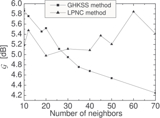
Figure 1: The plot of the gain parameter $\mathcal{G}$ versus number of iterations of the GHKSS method (squares) and LPNC method (triangles). Lorenz system $\mathcal{N}=78\%$, $N=1000$.

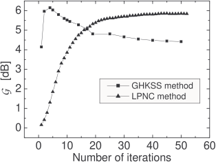
Figure 2: The plot of the gain parameter $\mathcal{G}$ versus number of neighbors of the GHKSS method (squares) and LPNC method (triangles). Lorenz system $\mathcal{N}=78\%$, $N=1000$.

If we consider uniformly distributed stochastic variables (see Fig. 3) the LPNC method reduces the noise very well, and as a result all data are represented as a neighborhood of a point attractor (see Fig. 4) while a complete noise reduction would correspond to a phase portrait consisting of a single point. In fact, for the case considered we observed for the LPNC method a noise reduction of about $96\%$ of data variance.

Figure 3: The random data from uniform distribution

Figure 4: The random data shown in the Fig. 3 after noise reduction with the LPNC method

V The Nearest neighborhood assessment

The LP methods are local. It follows that features of the nearest neighborhood $\mathbf{X}_{n}^{NN}$ of every point $\mathbf{x}_{n}$ in the phase space play an important role. Usually the nearest neighborhood is estimated by the smallest distance approach that makes use of the standard Euclidian geometry. We have found, however, that our LPNC method works much better when the Delaunay triangulation approach allie is applied for the nearest neighborhood estimation.

V.1 The smallest distance approach (SD)

In the smallest distance approach the Euclidian metric is used, i.e. first the distance between every pair of points in the Takens embedded space is calculated as $d_{i,j}=\sqrt{\left(x_{i}-x_{j}\right)^{2}+\ldots+\left(x_{i-\left(d-1\right)\tau}-x_{j-\left(d-1\right)\tau}\right)^{2}}$ and then the nearest neighborhood $\mathbf{X}_{n}^{NN}$ of a point $\mathbf{x}_{n}$ is defined as a set of $\nu$ points fulfilling the relation

$$\left\{\mathbf{x}_{j}\in\mathbf{X}_{n}^{NN},\forall_{k}\mathbf{x}_{k}\notin\mathbf{X}_{n}^{NN}:d_{n,j}\leq d_{n,k}\right\}.$$ (34)

Let us stress that this definition depends on the chosen value of the $\nu$ parameter. i.e. on the assumed number of near neighbors, $\nu=2,3,\ldots$.

V.2 The Delaunay triangulation approach (DT)

To find the nearest neighborhood relations for the LPNC method we have used the Delaunay triangulation allie . In general the triangulation of any set of points $\mathbf{X}=\left\{\mathbf{x}_{i}\right\}\in\mathbb{R}^{d}$ is a collection of $d$-dimensional simplices with disjoint interiors and vertices chosen from $\mathbf{X}$. There are many triangulation of the same set of points $\mathbf{X}$. One of the best known is the Delaunay triangulation (see Fig. 5). Let $T\left(\mathbf{x}_{n}\right)$ be a part of the space $\mathbb{R}^{d}$ that contains all points that are closer to $\mathbf{x}_{n}$ than any other point $\mathbf{x}_{j}$ from the set $\mathbf{X}$

$$T\left(\mathbf{x}_{n}\right)=\left\{z\in\mathbb{R}^{d},\mathbf{x}_{j}\in\mathbf{X}:\forall_{j\neq n}\left\|z-\mathbf{x}_{n}\right\|\leq\left\|z-\mathbf{x}_{j}\right\|\right\}.$$ (35)

If $\mathbf{m}_{i,j}=\left(\mathbf{x}_{i}+\mathbf{x}_{j}\right)/2$ belongs to both sets $T\left(\mathbf{x}_{i}\right)$ and $T\left(\mathbf{x}_{j}\right)$ then by definition the point $\mathbf{x}_{j}$ is the nearest neighbor of $\mathbf{x}_{i}$ received due to the Delaunay triangulation. By the above definition every point $\mathbf{x}_{n}$ belongs to its nearest neighborhood $\mathbf{x}_{n}\in\mathbf{X}_{n}^{NN}$.

In practice the Delaunay approach can be performed as follows. A pair of points $\mathbf{x}_{n}$ and $\mathbf{x}_{j}$ are near neighbors provided that there are no other points $\mathbf{x}_{k}$ ($k\neq j,n$) belonging to the hypersphere centered at the point $\mathbf{m}_{n,j}$ and of the radius $r_{n,j}=\left\|\mathbf{x}_{n}-\mathbf{x}_{j}\right\|/2$.

In Fig. 6 two cases are presented when in the two-dimensional space a) the point $\mathbf{x}_{j}$ is not the nearest neighbor of $\mathbf{x}_{n}$ and b) the point $\mathbf{x}_{j}$ is the nearest neighbor of $\mathbf{x}_{n}$.

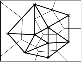
Figure 5: Delaunay triangulation for a set of nine points in a two-dimensional space. The near neighbors are connected by bold lines. Sets $T\left(\mathbf{x}_{i}\right)$, $i=1,2,\ldots,9$ are limited by thin lines.

Figure 6: Illustration of nearest neighborhood search by DT approach a) $\mathbf{x}_{j}$ and $\mathbf{x}_{n}$ are not near neighbors. b) $\mathbf{x}_{j}$ and $\mathbf{x}_{n}$ are near neighbors

.

The DT method has the advantage that triangles appearing due to connections of near neighbors are almost equiangular (see Fig. 5). This property is the main reason for using the DT method in search of the near neighbors. The disadvantage of this method is a slowing down of numerical calculations.

VI Examples of noise reductions

The LPNC method has been applied to three systems: the Henon map, the Lorenz model lorenz and the Chua circuit anischenko ; chua1 ; chua2 . Figures 7 - 9 present the chaotic Henon map in the absence and in the presence of measurement noise as well as a result of the noise reduction.

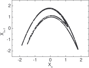
Figure 7: Chaotic Henon map without noise

Figure 8: Chaotic Henon map with a measurement noise $\mathcal{N}=69\%$. Note the difference in scale.

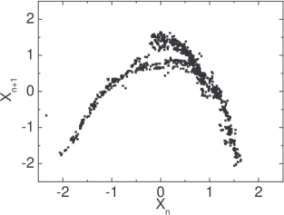
Figure 9: Chaotic Henon map with a measurement noise after noise reduction with the LPNC method, $\mathcal{G}=4.3$

Table 1 presents the values of the gain parameter for the Henon map and for the Lorenz system.

To verify our method in a real experiment we have performed the analysis of data generated by a nonlinear electronic circuit. The Chua circuit in the chaotic regime chua1 ; chua2 has been used and we have added a measurement noise to the outcoming signal. The noise (white and Gaussian) came from an electronic noise generator. Figures 10 - 12 show a clean signal coming from this circuit, the signal generated by Chua circuit with measurement noise ($\mathcal{N}=96.5\%$) and the same signal after the noise reduction with the LPNC method ($\mathcal{G}=6.38$). Table 2 presents values of the $\mathcal{G}$ parameter and the percentage of eliminated noise for several values of the noise level in the Chua circuit.

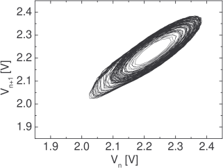
Figure 10: The stroboscopic map corresponding to a clean trajectory in the Chua circuit.

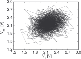
Figure 11: The stroboscopic map received from the Chua circuit in the presence of a measurement noise $\mathcal{N}=96.5\%$. Note the difference in scale.

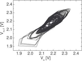
Figure 12: The stroboscopic map received after the noise reduction by the LPNC method applied to data presented at Fig. 11.

Table 1: Results of noise reduction by the LPNC method for the Henon map and Lorenz model.

System	$\mathcal{N}$	$\mathcal{G}$	percent. of eliminated noise
Henon $N=1000$	$10\%$	$9.58$	$89\%$
Henon $N=3000$	$10\%$	$10.04$	$91\%$
Henon $N=1000$	$66\%$	$5.08$	$69\%$
Lorenz $N=1000$	$78\%$	$5.85$	$74\%$
Lorenz $N=3000$	$76\%$	$6.02$	$75\%$
Lorenz $N=1000$	$34\%$	$7.21$	$81\%$

Table 2: Results of noise reduction by the LPNC method for the Chua circuit with a measurement noise ($N=3000$).

$\mathcal{N}$	$\mathcal{G}$	percent. of eliminated noise
$24.9\%$	5.4	71%
$28.3\%$	4.9	68%
$46.1\%$	7.0	80%
$73.7\%$	4.81	67%
$90.6\%$	7.4	82%
$96.5\%$	6.4	77%

All the above applications of the LPNC method consider the case of measurement noise that has been added to the signal in numerical or electronic experiments. However, our LPNC method can also be applied to dynamical noise i.e to the noise which in experiments is included in the equations of motion Jaeger . In such a case one cannot compare the noisy data with the clean trajectory since the latter one does not exist anymore, and there are only $\epsilon$-shadowed trajectories Farmer that can be approximated by means of the LPNC method. Figure 13 shows a measured signal generated by a Chua circuit where a mixture of measurement noise and dynamical noise occurs. Figure 14 shows the result of noise reduction applied to such a signal.

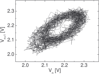
Figure 13: Stroboscopic map received from the Chua circuit in the presence of a mixture of a measurement and dynamical noise $\mathcal{N}\approx 22\%$.

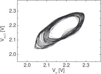
Figure 14: Stroboscopic map received after noise reduction by the LPNC method applied to data presented at Fig. 13

VII Noise level estimation by LPNC method

The LPNC method introduced in the previous section can be used to quantify the noise level of data. The noise level, i.e. the standard deviation in noisy time series, may be approximated as the Euclidian distance between the vectors $\left\{x_{i}\right\}$ and $\left\{\bar{x}_{i}\right\}$ representing the time series before and after noise reduction Hsu

$$\tilde{\sigma}_{noise}\approx\sqrt{\frac{1}{N}\sum\limits_{i=1}^{N}\left(x_{i}-\bar{x}_{i}\right)^{2}}.$$ (36)

The main disadvantage of the LPNC method used for the noise level estimation is its small rate of convergence with respect to other known methods urbanowicz ; Diks ; Yu ; Oltmans and the fact that the method can be used only for low-dimensional systems. On the other hand the LPNC method can be applied for estimation of any noise level including a large one. In Table 3 we have presented the estimated noise level $\tilde{\sigma}_{noise}$ for the Chua circuit.

Table 3: Noise level estimated by the LPNC method for the Chua circuit with measurement noise ($N=3000$).

$\mathcal{N}$	$\sigma_{noise}$ [mV]	$\tilde{\sigma}_{noise}$ [mV]
$0\%$	0	5.5
$3.1\%$	30.4	28.9
$6.2\%$	60.8	53.7
$12.3\%$	121.7	110
$24.9\%$	243.4	235
$28.3\%$	304	305
$46.1\%$	486	454
$73.7\%$	973	938
$90.6\%$	1520	1375
$96.5\%$	2120	1844

VIII Conclusions

In conclusion we have developed a method of noise reduction that makes use of nonlinear constraints which occur in a natural way due to the linearization of a deterministic system trajectory in the nearest neighborhood of every point in the phase space. This neighborhood has been determined by Delaunay triangulation. The method has been applied to data from the Henon map, Lorenz model and electronic Chua circuit contaminated by measurement (additive) noise. The efficiency of our method is comparable to that of standard LP methods but it is more robust to input parameter adjustment.

Appendix A Multidimensional version of LPNC method

In Sec. III the LPNC method has been presented for one-dimensional systems. Here we show the generalization of this approach for $d$-dimensional dynamics. For one-dimensional problems the Jacobi matrix of the system does not appear explicitly in our method. For higher dimensional models the corresponding Jacobian $\mathbf{A}$ has to be calculated but we manage to minimalize errors occurring by its estimation. The linearized equation of motion for vectors from the nearest neighborhood $\tilde{\mathbf{X}}_{n}^{NN}$ of a vector $\tilde{\mathbf{x}}_{n}$ can be written in the form

$$\tilde{\mathbf{x}}_{n+1}=\mathbf{A}\cdot\tilde{\mathbf{x}}_{n}+\mathbf{b}.$$ (37)

In such a case one needs three vectors $\tilde{\mathbf{x}}_{n},\tilde{\mathbf{x}}_{k},\tilde{\mathbf{x}}_{j}\in\tilde{\mathbf{X}}_{n}^{NN}$ to write constraints corresponding to Eq. (13). In comparison with to the one-dimensional case the number of near neighbors i.e. the number of points in the set $\tilde{\mathbf{X}}_{n}^{NN}$ must be larger to allow a unique estimation of the Jacobian $\mathbf{A}$. We assume that the Jacobi matrix can be approximately received by minimalization of the following cost functional

$$\sum_{s}(a_{m1}x_{s}+a_{m2}x_{s-\tau}+\ldots$$

$$\ldots+a_{md}x_{s-\left(d-1\right)\tau}-x_{s+1-m\tau})^{2}=min$$

$$(\forall_{m=1,\ldots,d})\quad\mbox{and}\quad\left\{s:\mathbf{x}_{s}\in\mathbf{X}_{n}^{NN}\right\},$$ (38)

where $a_{ij}=\left[\mathbf{A}\right]_{ij}$. By analogy with Eq. (13) we introduce the follow

$$G_{m}^{d}\left(\tilde{\mathbf{X}}_{n}^{NN}\right)\equiv a_{m1}G\left(\tilde{\mathbf{X}}_{n}^{NN},\mathbf{\tilde{X}}_{n+1-m\tau}\right)+$$

$$a_{m2}G\left(\mathbf{\tilde{X}}_{n-\tau},\mathbf{\tilde{X}}_{n+1-m\tau}\right)+\ldots$$

$$\ldots+a_{md}G\left(\mathbf{\tilde{X}}_{n-\left(d-1\right)\tau},\mathbf{\tilde{X}}_{n+1-m\tau}\right)=0$$

$$\quad(\forall_{m=1,\ldots,d}),$$ (39)

where we used the notation corresponding to equation (17) i.e.

$$G\left(\mathbf{X}_{n}^{NN},\mathbf{X}_{n+l}\right)=x_{n}\left(x_{k+l}-x_{j+l}\right)+x_{k}\left(x_{j+l}-x_{n+l}\right)+x_{j}\left(x_{n+l}-x_{k+l}\right)$$

$$G\left(\mathbf{X}_{n-s},\mathbf{X}_{n+l}\right)=x_{n-s}\left(x_{k+l}-x_{j+l}\right)+x_{k-s}\left(x_{j+l}-x_{n+l}\right)+x_{j-s}\left(x_{n+l}-x_{k+l}\right),$$ (40)

$\mathbf{X}_{n+s}=\left\{\mathbf{x}_{n+s},\mathbf{x}_{k+s},\mathbf{x}_{j+s}\right\}\quad(\forall_{s=0,\pm 1,\pm 2,\ldots})$ where $\left\{n,j,k:\mathbf{x}_{n},\mathbf{x}_{k},\mathbf{x}_{j}\in\mathbf{X}_{n}^{NN}\right\}$. Since the clean trajectory is not known thus in the Eq. (39) the observed variables $\mathbf{X}_{n}^{NN}$, $\mathbf{X}_{n+1-m\tau}$ etc. are used.

In such a way the equation (20) can be written in a more general way as

$$\sum_{l=1}^{d}a_{ml}G\left(\delta\mathbf{X}_{n-\left(l-1\right)\tau},\delta\mathbf{X}_{n+1-m\tau}\right)\cong 0$$

$$\quad(\forall_{n=1,\ldots,N},\forall_{m=1,\ldots,d})$$ (41)

where we use

$$G\left(\delta\mathbf{X}_{n-s},\delta\mathbf{X}_{n+l}\right)=\delta x_{n-s}\left(\delta x_{k+l}-\delta x_{j+l}\right)$$

$$+\delta x_{k-s}\left(\delta x_{j+l}-\delta x_{n+l}\right)+\delta x_{j-s}\left(\delta x_{n+l}-\delta x_{k+l}\right)$$ (42)

$\delta\mathbf{X}_{n+s}=\left\{\delta\mathbf{x}_{n+s},\delta\mathbf{x}_{k+s},\delta\mathbf{x}_{j+s}\right\}\quad(\forall_{s=0,\pm 1,\pm 2,\ldots})$, where $\left\{n,j,k:\mathbf{x}_{n},\mathbf{x}_{k},\mathbf{x}_{j}\in\mathbf{X}_{n}^{NN}\right\}$, $\delta\mathbf{x}_{n}=\left\{\delta x_{n},\delta x_{n-\tau},\ldots,\delta x_{n-\left(d-1\right)\tau}\right\}\quad\mbox{and}\quad\left\{n:\mathbf{x}_{n}\in\mathbf{X}_{n}^{NN}\right\}$.

Now the cost problem (22) can be transformed to the form

$$\tilde{S}_{n}^{NN}=\sum_{s}\left(\delta x_{s}\right)^{2}+\lambda_{n}^{m}G_{m}^{d}\left(\mathbf{X}_{n}^{NN}\right)=min$$

$$(\forall_{n=1,...,N},\forall_{m=1,\ldots,d})$$

$$\quad\mbox{and}\quad\left\{s:\mathbf{x}_{s}\in\mathbf{X}_{n}^{NN}\;\mbox{or}\;\mathbf{x}_{s}\in\mathbf{X}_{n+1}\right\}.$$ (43)

Finding zeros of partial derivatives of the functional (43) one can linearize this problem and write it in the form similar to the Eq. (23)

$$\mathbf{M}_{n}\cdot\delta\mathbf{X}_{n}^{\lambda}=\mathbf{B}_{n}\quad(\forall_{n=1,\ldots,N}).$$ (44)

Vectors $\delta\mathbf{X}_{n}^{\lambda}$ and $\mathbf{B}_{n}$ occurring in Eq. (44) are equal to

$$\left(\delta\mathbf{X}_{n}^{\lambda}\right)^{T}=\{\delta x_{n-\left(d-1\right)\tau},\delta x_{n-\left(d-2\right)\tau},\ldots$$

$$\ldots,\delta x_{n},\delta x_{n+1},\lambda_{n}^{1},\lambda_{n}^{2},\ldots,\lambda_{n}^{d}\},$$ (45)

$$\mathbf{B}_{n}^{T}=\{0,0,\ldots,0,-G_{1}^{d}\left(\mathbf{X}_{n}^{NN}\right),-G_{2}^{d}\left(\mathbf{X}_{n}^{NN}\right),\ldots$$

$$\ldots,-G_{d}^{d}\left(\mathbf{X}_{n}^{NN}\right)\}$$ (46)

where the number of zeros $d_{0}$ appearing in $\mathbf{B}_{n}^{T}$ depends on the values of $\tau$ and $d$ and for the case $\tau=1$, $d_{0}=d+1$. Elements of the matrix $\mathbf{M}_{n}$ can be written as

$$\left[\mathbf{M}_{n}\right]_{mm} = 2\quad(\forall_{m=1,\ldots,d_{0}})$$

$$\left[\mathbf{M}_{n}\right]_{lm} = \left[\mathbf{M}_{n}\right]_{ml}+=\sum_{s=1}^{d}a_{ms}\left(x_{k+1}-x_{j+1}\right)\quad(\forall_{m=d_{0}+1,\ldots,d_{0}+d+1})\quad\mbox{and}\quad\left\{l:x_{l}\in\mathbf{x}_{n}\right\}$$

$$\left[\mathbf{M}_{n}\right]_{lm} = \left[\mathbf{M}_{n}\right]_{ml}+=\sum_{s=1}^{d}a_{ms}\left(x_{j+1}-x_{n+1}\right)\quad(\forall_{m=d_{0}+1,\ldots,d_{0}+d+1})\quad\mbox{and}\quad\left\{l:x_{l}\in\mathbf{x}_{k}\right\}$$

$$\left[\mathbf{M}_{n}\right]_{lm} = \left[\mathbf{M}_{n}\right]_{ml}+=\sum_{s=1}^{d}a_{ms}\left(x_{n+1}-x_{k+1}\right)\quad(\forall_{m=d_{0}+1,\ldots,d_{0}+d+1})\quad\mbox{and}\quad\left\{l:x_{l}\in\mathbf{x}_{j}\right\}$$ (47)

$$\left[\mathbf{M}_{n}\right]_{lm} = \left[\mathbf{M}_{n}\right]_{ml}+=\sum_{s=1}^{d}a_{ms}\left(x_{j-m\tau}-x_{k-m\tau}\right)\quad(\forall_{m=d_{0}+1,\ldots,d_{0}+d+1})\quad\mbox{and}\quad\left\{l:x_{l}\in\mathbf{x}_{n+1}\right\}$$

$$\left[\mathbf{M}_{n}\right]_{lm} = \left[\mathbf{M}_{n}\right]_{ml}+=\sum_{s=1}^{d}a_{ms}\left(x_{n-m\tau}-x_{j-m\tau}\right)\quad(\forall_{m=d_{0}+1,\ldots,d_{0}+d+1})\quad\mbox{and}\quad\left\{l:x_{l}\in\mathbf{x}_{k+1}\right\}$$

$$\left[\mathbf{M}_{n}\right]_{lm} = \left[\mathbf{M}_{n}\right]_{ml}+=\sum_{s=1}^{d}a_{ms}\left(x_{k-m\tau}-x_{n-m\tau}\right)\quad(\forall_{m=d_{0}+1,\ldots,d_{0}+d+1})\quad\mbox{and}\quad\left\{l:x_{l}\in\mathbf{x}_{j+1}\right\}$$

where the remaining $\mathbf{M}_{n}$ elements vanish and $x_{l}\in\mathbf{x}_{n}$ means that the variable $x_{l}$ is a component of the $\mathbf{x}_{n}$ vector.

The operator $+=$ in (47) has the same meaning as in the programming language C++, i.e. if elements of the matrix $\left[\mathbf{M}_{n}\right]_{ml}$ occur in a few places (e.g. : $x_{n}\in\mathbf{x}_{n}\;\mbox{and}\;x_{n}\in\mathbf{x}_{n+1}\quad\forall_{d>1},\vee_{\tau=1}$) then the elements at the rhs of such equations have to be summed up.

References

• (1) H. Kantz and T. Schreiber, Nonlinear Time Series Analysis (Cambridge University Press, Cambridge, 1997).
• (2) H.D.I. Abarbanel, Analysis of Observed Chaotic Data (Springer, New York, 1996).
• (3) T. Kapitaniak, Chaos in Systems with Noise (World Scientific, Singapore, 1990).
• (4) K. Urbanowicz and J. A. Hołyst, Phys. Rev. E 67, 046218 (2003).
• (5) E.J. Kostelich and T. Schreiber, Phys. Rev. E 48(3),1752 (1993).
• (6) T. Schreiber, Phys. Rev. E 48(1),13(4) (1993).
• (7) T. Schreiber, Phys. Rev. E 47(4),2401 (1992).
• (8) J. D. Farmer and J.J. Sidorowich, Physica D 47, 373-392 (1991).
• (9) S.M. Hammel, Phys. Lett. A 148, 421 (1990).
• (10) M.E. Davies, Physica D 79, 174 (1994).
• (11) X.P. Zhang, IEEE Trans. Neural Networ. 12(3), 567 (2001).
• (12) X.R. Chen and S. Tokinaga, IEICE Trans. Fund. Electr. E85A(9), 2107 (2002).
• (13) P. Grassberger and I. Procaccia, Phys. Rev. Lett. 50(5), 346 (1983).
• (14) S.J. Julier, J.K. Uhlmann and H.F. Durrans-Whyte, IEEE Trans. on Autom. Contr. 5(3), 477 (2000).
• (15) A. Effern, K. Lehnertz, T. Schreiber, T. Grunwald, P. David and C.E. Elger, Physica D 140, 247 (2000).
• (16) R. Cawley and G. H. Hsu, Phys. Rev. A 46(6), 3057 (1992).
• (17) T. Sauer, Physica D 58, 193 (1994).
• (18) P. Grassberger, R. Hegger, H. Kantz, C. Schaffrath and T. Schreiber, Chaos 3(2),127 (1993).
• (19) D. Broomhead and D. Lowe, Complex Syst. 2, 321 (1988).
• (20) L. Matassini, H. Kantz, J. Holyst, and R. Hegger, Phys. Rev. E 65, 021102 (2002).
• (21) S. Allie, A. Mees, K. Judd and D. Watson, Phys. Rev. E 55(1),87(7) (1997).
• (22) E.N. Lorenz, J. Atmos. Sci. 20, 130 (1963).
• (23) S. Wu, Proceedings of the IEEE, vol. 75, No. 8 (1987).
• (24) L.O Chua and G.-N. Lin, IEEE Trans. Circuits Syst. 37(7),885-902 (1990).
• (25) V.S. Anishchenko, M.A. Safonova and L.O. Chua, Journ. Circuits Syst. Comp. 3(2), 553-578 (1993).
• (26) L. Jaeger and H. Kantz, Physica D 105, 79-96 (1997).
• (27) C. Diks, Phys. Rev. E 53(5),4263(4) (1996).
• (28) D. Yu, M. Small, R.G. Harrison and C. Diks, Phys. Rev. E 61(4),3750(7) (2000).
• (29) H. Oltmans and P. J. T. Verheijen, Phys. Rev. E 56(1),1160(11) (1997).